跳到论文正文
W Papers独立论文阅读器 arXiv:1909.11518 论文正文 计算阅读时间 · 0%
引用这篇论文根据当前论文元数据生成,正式投稿前建议核对。


License: arXiv.org perpetual non-exclusive license
arXiv:1909.11518v3 [math.PR] 13 Nov 2019

Distances between distributions via Stein’s method

Marie Ernst11 1 Université de Liège.    Yvik Swan22 2 Université libre de Bruxelles.
August 11, 2026

We build on the formalism developed in [21] to propose new representations of solutions to Stein equations. We provide new uniform and non uniform bounds on these solutions (a.k.a. Stein factors). We use these representations to obtain representations for differences between expectations in terms of solutions to the Stein equations. We apply these to compute abstract Stein-type bounds on Kolmogorov, Total Variation and Wasserstein distances between arbitrary distributions. We apply our results to several illustrative examples, and compare our results with current literature on the same topic, whenever possible. In all occurrences our results are competitive.

Keywords: Stein’s method, Stein equations, Stein factors, Kolmogorov distance, Wasserstein distance, Total variation distance, Integral probability metrics.

1 Introduction

Consider two random variables Xn,X∞∈I​RX_{n},X_{\infty}\in{\rm I\kern-1.60004ptR} such that ℒ⁡(Xn)≈ℒ⁡(X∞)\mathcal{L}(X_{n})\approx\mathcal{L}(X_{\infty}). It is of course of great importance to be able to quantify this proximity in terms of a relevant quantity 𝒟⁡(Xn,X∞)\mathcal{D}(X_{n},X_{\infty}), say. The literature contains many such discrepancy metrics, including Hellinger, Lévy, Prokhorov, ff-divergences, relative entropy, … See e.g. [26] for an overview. In this paper we shall focus on the following three:

  • •

    Kolmogorov distance: Kol⁡(Xn,X∞)=supz∈I​R|ℙ⁡(Xn≤z)−ℙ⁡(X∞≤z)|\mathrm{Kol}(X_{n},X_{\infty})=\sup_{z\in{\rm I\kern-1.27557ptR}}\left|\mathbb{P}(X_{n}\leq z)-\mathbb{P}(X_{\infty}\leq z)\right|

  • •

    Total Variation distance: TV⁡(Xn,X∞)=supB⊂I​R|ℙ⁡(Xn∈B)−ℙ⁡(X∞∈B)|\mathrm{TV}(X_{n},X_{\infty})=\sup_{B\subset{\rm I\kern-1.27557ptR}}\left|\mathbb{P}(X_{n}\in B)-\mathbb{P}(X_{\infty}\in B)\right|

  • •

    Wasserstein distance: Wass⁡(Xn,X∞)=∫−∞∞|ℙ⁡(Xn≤z)−ℙ⁡(X∞≤z)|​𝑑z\mathrm{Wass}(X_{n},X_{\infty})=\int_{-\infty}^{\infty}\left|\mathbb{P}(X_{n}\leq z)-\mathbb{P}(X_{\infty}\leq z)\right|\mathrm{d}z

It is generally non-trivial to determine bounds L1≤𝒟⁡(Xn,X∞)≤L2L_{1}\leq\mathcal{D}(X_{n},X_{\infty})\leq L_{2} with L1,L2L_{1},L_{2} meaningful and computable quantities. Such bounds typically depend on the choice of metric, as well as the nature of the “target” law (ℒ⁡(X∞)\mathcal{L}(X_{\infty}), say) and of the “approximating” law (ℒ⁡(Xn)\mathcal{L}(X_{n}), say). Famous examples include the following:

Example 1.1 (Berry-Esseen bound ∼\sim 1942).

Let Xn=n−1/2∑i=1nXiX_{n}=n^{-1/2}\sum_{i=1}^{n}X_{i} with XiX_{i} iid mean 0 variance 1 and X∞∼𝒩⁡(0,1)X_{\infty}\sim\mathcal{N}(0,1). Then Kol(Xn,X∞)≤Cn−1/2𝔼[|X1|3]{\mathrm{Kol}(X_{n},X_{\infty})\leq{C}{n^{-1/2}}\mathbb{E}\big[|X_{1}|^{3}\big]} for C∈(0.40973,0.4748)C\in(0.40973,0.4748).

Example 1.2 (Le Cam’s inequality ∼\sim 1960).

Let Xn=∑i=1nXiX_{n}=\sum_{i=1}^{n}X_{i} with Xi∼indBern⁡(θi)X_{i}\stackrel{{\scriptstyle\mathrm{ind}}}{{\sim}}\mathrm{Bern}(\theta_{i}) and X∞∼Poi⁡(λ)X_{\infty}\sim\mathrm{Poi}(\lambda) with λ=∑i=1nθi\lambda=\sum_{i=1}^{n}\theta_{i}. Here and throughout we write a∧b=min⁡(a,b)a\wedge b=\min(a,b) and a∨b=max⁡(a,b)a\lor b=\max(a,b). Then (1∧λ−1)​∑i=1nθi2/32≤TV⁡(Xn,X∞)≤(1−e−λ)​λ−1​∑i=1nθi2{(1\wedge{\lambda}^{-1})\sum_{i=1}^{n}\theta_{i}^{2}/32\leq\mathrm{TV}(X_{n},X_{\infty})\leq({1-e^{-\lambda}}){\lambda}^{-1}\sum_{i=1}^{n}\theta_{i}^{2}}.

Examples 1.1 and 1.2 illustrate situations wherein the target law is easy and explicit while the approximating is unknown and unfathomable. There is also interest for situations wherein both the target and the approximating distributions are known explicitly.

Example 1.3 ([17]).
  • •

    TV⁡(Hyp⁡(N,L,n),Bin⁡(n,L/N))≤(n−1)/N.\mathrm{TV}(\mathrm{Hyp}(N,L,n),\mathrm{Bin}(n,L/N))\leq(n-1)/N.

  • •

    TV⁡(Bin⁡(n,λ/n),Poi⁡(λ))≤1−(1−⌈λ⌉n)1/2.\mathrm{TV}(\mathrm{Bin}(n,\lambda/n),\mathrm{Poi}(\lambda))\leq 1-\left(1-\frac{\lceil\lambda\rceil}{n}\right)^{1/2}.

  • •

    TV⁡(Beta⁡(a,b),Gamma⁡(a,a+b))≤1−(1−a+1a+b)1/2\mathrm{TV}(\mathrm{Beta}(a,b),\mathrm{Gamma}(a,a+b))\leq 1-\left(1-\frac{a+1}{a+b}\right)^{1/2}

There are many ways to prove estimates such as those provided in Examples 1.1, 1.2, and 1.3, such as Fourier methods, couplings or, whenever possible, direct analysis of the densities involved. In this paper we will consider the well-known Stein’s method. Our approach builds upon recent results from [21, 22]. In those papers it is shown that one can associate to any X∞X_{\infty} two linear operators 𝒯∞ℓ\mathcal{T}_{\infty}^{\ell} and ℒ∞ℓ\mathcal{L}_{\infty}^{\ell} such that the “Stein identities”

Cov⁡[f⁡(X∞),g⁡(X∞)]=𝔼⁡[−ℒ∞ℓ​f​(X∞)​Δ−ℓ​g​(X∞)]\displaystyle\mathrm{Cov}[f(X_{\infty}),g(X_{\infty})]=\mathbb{E}\left[-\mathcal{L}_{\infty}^{\ell}f(X_{\infty})\Delta^{-\ell}g(X_{\infty})\right] (1.1)
𝔼⁡[(𝒯∞ℓ​f​(X∞))​g​(X∞)]=−𝔼⁡[f⁡(X∞)​Δ−ℓ​g​(X∞)]\displaystyle\mathbb{E}\left[\big(\mathcal{T}_{\infty}^{\ell}f(X_{\infty})\big)g(X_{\infty})\right]=-\mathbb{E}\left[f(X_{\infty})\Delta^{-\ell}g(X_{\infty})\right] (1.2)

are valid for all sufficiently regular functions f,gf,g (here Δ−ℓ\Delta^{-\ell} is a generalized differential operator, see Section 2.1 for explicit expressions).

Example 1.4.

Take X∞X_{\infty} standard Gaussian with density φ(x)=(2π)−1e−x2/2\varphi(x)=(2\pi)^{-1}e^{-x^{2}/2}. Then ℓ=0\ell=0, 𝒯∞0​f​(x)=f′​(x)−x​f​(x)\mathcal{T}_{\infty}^{0}f(x)=f^{\prime}(x)-xf(x), ℒ∞​f​(x)=ex2/2​∫−∞x(f⁡(u)−𝔼⁡[f⁡(X∞)])​𝑑u\mathcal{L}_{\infty}f(x)=e^{x^{2}/2}\int_{-\infty}^{x}(f(u)-\mathbb{E}[f(X_{\infty})])\mathrm{d}u, so that (1.1) and (1.2) read as

Cov[f(X∞),g(X∞)]=𝔼[(eX∞2/2∫−∞X∞(𝔼[f(X∞)]−f(u))e−u2/2du)g′(X∞)]\displaystyle\mathrm{Cov}[f(X_{\infty}),g(X_{\infty})]=\mathbb{E}\left[\left(e^{X_{\infty}^{2}/2}\int_{-\infty}^{X_{\infty}}(\mathbb{E}[f(X_{\infty})]-f(u))e^{-u^{2}/2}\mathrm{d}u\right)g^{\prime}(X_{\infty})\right]
𝔼⁡[(f′​(X∞)−X∞​f​(X∞))​g​(X∞)]=−𝔼⁡[f⁡(X∞)​g′​(X∞)]\displaystyle\mathbb{E}\left[\big(f^{\prime}(X_{\infty})-X_{\infty}f(X_{\infty})\big)g(X_{\infty})\right]=-\mathbb{E}\left[f(X_{\infty})g^{\prime}(X_{\infty})\right]

which hold for all f∈L1​(φ)f\in L^{1}(\varphi) and absolutely continuous functions gg. Both identities are a straightforward consequence of Fubini’s theorem.

If, in (1.1) or (1.2), we take expectations with respect to XnX_{n} rather than X∞X_{\infty}, absence of equality in either identities for some functions f,gf,g indicates absence of equality between the laws of XnX_{n} and X∞X_{\infty}. Stein’s method consists in transforming this observation into estimates on relevant probability distances between the laws of XnX_{n} and X∞X_{\infty}. More precisely, the method advocates to fix ff in (1.1) or (1.2) some “well chosen” function (e.g. f⁡(x)=1f(x)=1, but this is not always ideal) and use the numbers

𝒮A​(Xn,X∞,𝒢):=supg∈𝒢|Cov⁡[f⁡(Xn),g⁡(Xn)]+𝔼⁡[(ℒ∞ℓ​f​(Xn))​Δ−ℓ​g​(Xn)]|\displaystyle\mathcal{S}_{A}(X_{n},X_{\infty},\mathcal{G}):=\sup_{g\in\mathcal{G}}\left|\mathrm{Cov}[f(X_{n}),g(X_{n})]+\mathbb{E}\left[\big(\mathcal{L}_{\infty}^{\ell}f(X_{n})\big)\Delta^{-\ell}g(X_{n})\right]\right|
𝒮B​(Xn,X∞,𝒢):=supg∈𝒢|𝔼⁡[(𝒯∞ℓ​f​(Xn))​g​(Xn)+f⁡(Xn)​Δ−ℓ​g​(Xn)]|\displaystyle\mathcal{S}_{B}(X_{n},X_{\infty},\mathcal{G}):=\sup_{g\in\mathcal{G}}\left|\mathbb{E}\left[\big(\mathcal{T}_{\infty}^{\ell}f(X_{n})\big)g(X_{n})+f(X_{n})\Delta^{-\ell}g(X_{n})\right]\right|

(with 𝒢\mathcal{G} “some class of functions” to be determined) to quantify the difference between the laws of XnX_{n} and X∞X_{\infty}.

Example 1.5.

If X∞X_{\infty} is standard normal, fixing f⁡(x)=xf(x)=x in (1.1) (or f⁡(x)=1f(x)=1 in (1.2)) leads to the discrepancy measure supg∈𝒢|𝔼⁡[g′​(Xn)−Xn​g​(Xn)]|\sup_{g\in\mathcal{G}}\left|\mathbb{E}[g^{\prime}(X_{n})-X_{n}g(X_{n})]\right| which, in light of Stein’s characterization of the normal distributon, is 0 if and only if XnX_{n} is itself Gaussian – at least when 𝒢\mathcal{G} is a sufficiently large class of test functions. Other choices of ff are possible, see [27].

Before diving into the study of the numbers 𝒮∙​(Xn,X∞,𝒢)\mathcal{S}_{\bullet}(X_{n},X_{\infty},\mathcal{G}), it is first necessary to argue as to why such numbers indeed metrize convergence in distribution in terms of relevant metrics. To this end, it suffices to notice that discrepancies 𝒮∙​(Xn,X∞,𝒢)\mathcal{S}_{\bullet}(X_{n},X_{\infty},\mathcal{G}) contain (at least formally) any distance that can be represented as an Integral Probability Metric (IPM):

𝒟ℋ​(Xn,X∞)=suph∈ℋ|𝔼​h​(Xn)−𝔼​h​(X∞)|.\mathcal{D}_{\mathcal{H}}(X_{n},X_{\infty})=\sup_{h\in\mathcal{H}}|\mathbb{E}h(X_{n})-\mathbb{E}h(X_{\infty})|. (1.3)

To see why this holds true, fix f=ηf=\eta in (1.1) or f=cf=c in (1.2) (the difference in notation is cosmetic but will help at a later stage) and consider the Stein equations

(η⁡(x)−𝔼​η​(X∞))​gh​(x)+(ℒ∞ℓ​η​(x))​Δ−ℓ​gh​(x)=h⁡(x)−𝔼​h​(X∞)\displaystyle(\eta(x)-\mathbb{E}\eta(X_{\infty}))g_{h}(x)+\big(\mathcal{L}_{\infty}^{\ell}\eta(x)\big)\Delta^{-\ell}g_{h}(x)=h(x)-\mathbb{E}h(X_{\infty}) (1.4)
𝒯∞ℓ​c​(x)​gh∗​(x)+c⁡(x)​Δ−ℓ​gh∗​(x)=h⁡(x)−𝔼​h​(X∞)\displaystyle\mathcal{T}_{\infty}^{\ell}c(x)g_{h}^{*}(x)+c(x)\Delta^{-\ell}g_{h}^{*}(x)=h(x)-\mathbb{E}h(X_{\infty}) (1.5)

for all x∈𝒮⁡(p∞)x\in\mathcal{S}(p_{\infty}). Lemma 2.11 in [21] guarantees that if ℋ\mathcal{H} is reasonable, then for any well-chosen η\eta or cc, to every h∈ℋh\in\mathcal{H} we can associate (uniquely) a function ghg_{h} or gh∗g_{h}^{*} such that either (1.4) or (1.5) holds at all xx in the support of the law of X∞X_{\infty}. Let 𝒢ℋ={gh|h∈ℋ}\mathcal{G}_{\mathcal{H}}=\left\{g_{h}\,|\,h\in\mathcal{H}\right\} and 𝒢ℋ∗={gh⋆|h∈ℋ}\mathcal{G}^{*}_{\mathcal{H}}=\left\{g_{h}^{\star}\,|\,h\in\mathcal{H}\right\} be the collection of all these solutions. Then simple computations show that

𝒟ℋ​(Xn,X∞)=𝒮A​(Xn,X∞,𝒢ℋ)=𝒮B​(Xn,X∞,𝒢ℋ∗).\mathcal{D}_{\mathcal{H}}(X_{n},X_{\infty})=\mathcal{S}_{A}(X_{n},X_{\infty},\mathcal{G}_{\mathcal{H}})=\mathcal{S}_{B}(X_{n},X_{\infty},\mathcal{G}^{*}_{\mathcal{H}}).

In other words, under non-stated regularity conditions which basically require that all quantities be defined, the IPMs (1.3) can be interpreted as specific instances of Stein’s discrepancies 𝒮∙\mathcal{S}_{\bullet}.

Example 1.6.

Still in the case where X∞X_{\infty} is standard Gaussian, fix η=Id\eta=\mathrm{Id} the identity function in (1.4) (or, equivalently, c=1c=1 in (1.5)) and consider the Stein equation

g′​(x)−x​g​(x)=h⁡(x)−𝔼​h​(X∞)g^{\prime}(x)-xg(x)=h(x)-\mathbb{E}h(X_{\infty}) (1.6)

over x∈ℝx\in\mathbb{R}. For each h∈L1​(X∞)h\in L^{1}(X_{\infty}) there exists a unique bounded solution given by gh​(x)=ex2/2​∫−∞x(h⁡(u)−𝔼​h​(X∞))​eu2/2​𝑑ug_{h}(x)=e^{x^{2}/2}\int_{-\infty}^{x}(h(u)-\mathbb{E}h(X_{\infty}))e^{u^{2}/2}\mathrm{d}u (we recognize the operator −ℒ∞0-\mathcal{L}_{\infty}^{0} from the previous example), so that

𝒟ℋ​(Xn,X∞)=suph∈ℋ|𝔼⁡[gh′​(Xn)−Xn​gh​(Xn)]|\displaystyle\mathcal{D}_{\mathcal{H}}(X_{n},X_{\infty})=\sup_{h\in\mathcal{H}}\left|\mathbb{E}[g_{h}^{\prime}(X_{n})-X_{n}g_{h}(X_{n})]\right|

and all IPMs with Gaussian target are indeed Stein discrepancies.

Many classical metrics can be represented as IPMs, most notably for us the Kolmogorov, Total Variation and Wasserstein distances with respective classes

ℋKol={h(x)=𝕀[x∈(−∞,z]] such that z∈ℝ}\displaystyle\mathcal{H}_{\mathrm{Kol}}=\left\{h(x)=\mathbb{I}[x\in(-\infty,z]]\mbox{ such that }z\in\mathbb{R}\right\}
ℋTV={h(x)=𝕀[x∈B] such that B∈ℬ(ℝ)}\displaystyle\mathcal{H}_{\mathrm{TV}}=\left\{h(x)=\mathbb{I}[x\in B]\mbox{ such that }B\in\mathcal{B}(\mathbb{R})\right\}
ℋWass=Lip⁡(1)={h⁡(x)​ such that ​|h⁡(x)−h⁡(y)|≤|x−y|​ for all ​x,y∈ℝ}\displaystyle\mathcal{H}_{\mathrm{Wass}}=\mathrm{Lip}(1)=\left\{h(x)\mbox{ such that }|h(x)-h(y)|\leq|x-y|\mbox{ for all }x,y\in\mathbb{R}\right\}

To summarize what has just been written, the heuristic behind our version of Stein’s method for a metric of the form (1.3) is to tackle the problem of bounding an IPM by contemplating the identities

𝒟ℋ​(Xn,X∞)\displaystyle\mathcal{D}_{\mathcal{H}}(X_{n},X_{\infty}) =suph∈ℋ|𝔼⁡[(η⁡(x)−𝔼​η​(X∞))​gh​(x)+(ℒ∞ℓ​η​(x))​Δ−ℓ​gh​(x)]|\displaystyle=\sup_{h\in\mathcal{H}}\left|\mathbb{E}\left[(\eta(x)-\mathbb{E}\eta(X_{\infty}))g_{h}(x)+\big(\mathcal{L}_{\infty}^{\ell}\eta(x)\big)\Delta^{-\ell}g_{h}(x)\right]\right|
=suph∈ℋ|𝔼⁡[𝒯∞ℓ​c​(Xn)​gh​(Xn)+c⁡(Xn)​Δ−ℓ​gh​(Xn)]|\displaystyle=\sup_{h\in\mathcal{H}}\left|\mathbb{E}\left[\mathcal{T}_{\infty}^{\ell}c(X_{n})g_{h}(X_{n})+c(X_{n})\Delta^{-\ell}g_{h}(X_{n})\right]\right|

where gh​(x)g_{h}(x) is solution to either (1.4) (first case) or (1.5) (second case). It remains of course to be able to choose η\eta or cc in such a way that the resulting expressions are tractable and the corresponding solutions ghg_{h} are well behaved.

It is now extremely well documented that, for many classical targets (particularly the normal and Poisson), this approach is powerful because there are many handles for dealing with the quantities 𝒮∙\mathcal{S}_{\bullet}, be it via exchangeable pairs, zero- and size bias, Malliavin-Stein, etc. We refer the reader to [2], [11] and [33] (among many other possible references) for an in-depth overview of a broad variety of applications around the Gaussian and Poisson cases. In this paper, we adopt the abstract formalism developed in [21, 22] to provide a new point of view on the properties of the solutions to equations (1.4) and (1.5). Our results are of two main types.

  • •

    The first, developed in Section 2.3, is of a classical nature within the theory on Stein’s method, and summarized in Proposition 2.27: we provide explicit uniform and non-uniform bounds on the solutions to Stein equations and on their derivatives. In all the examples we have considered, our bounds are easily computed and competitive with existing bounds (whenever there are competitors available). For instance, applying our bounds to the Gaussian case leads (see Example 2.31) to the fact that the solutions to equation (1.6) satisfy

    |g⁡(x)|≤min⁡(κ1​Φ​(x)​(1−Φ​(x))φ⁡(x),κ2)≤min⁡(κ1​12​π2,κ2)\displaystyle|g(x)|\leq\min\left(\kappa_{1}\frac{\Phi(x)(1-\Phi(x))}{\varphi(x)},\kappa_{2}\right)\leq\min\left(\kappa_{1}\frac{1}{2}\sqrt{\frac{\pi}{2}},\kappa_{2}\right)
    |g′​(x)|≤κ1​(1+|x|​Φ​(x)​(1−Φ​(x))φ⁡(x))≤2​κ1\displaystyle|g^{\prime}(x)|\leq\kappa_{1}\left(1+|x|\frac{\Phi(x)(1-\Phi(x))}{\varphi(x)}\right)\leq 2\kappa_{1}
    |g′​(x)|≤2​κ2​min⁡(|x|,∫−∞xΦ⁡(u)​𝑑u​∫x∞(1−Φ⁡(u))​𝑑uφ⁡(x))≤2​κ2​min⁡(2π,|x|)\displaystyle|g^{\prime}(x)|\leq 2\kappa_{2}\min\left(|x|,\frac{\int_{-\infty}^{x}\Phi(u)\mathrm{d}u\int_{x}^{\infty}(1-\Phi(u))\mathrm{d}u}{\varphi(x)}\right)\leq 2\kappa_{2}\min\left(\sqrt{\frac{2}{\pi}},|x|\right)

    where Φ\Phi is the standard normal cdf, κ1≤2​‖h‖∞\kappa_{1}\leq 2\|h\|_{\infty} and κ2≤‖h′‖∞\kappa_{2}\leq\|h^{\prime}\|_{\infty}. In the body of the article we also compute the bounds the Poisson (Example 2.33) and the exponential (Example 2.32). Other targets are covered in the supplementary material to this article.

  • •

    Our second main result is developed in Section 3, where we propose probabilistic representations of differences between expectations which allow to dispense with the need to bound solutions to Stein equations. As applications we provide new representations for (and bounds on) the Kolmogorov, Total Variation and Wasserstein distances whenever the target and the approximating random variables are continuous w.r.t. the same dominating measure. For instance in the case of a Gaussian target we obtain (see Example 3.7) that if Xn∼pnX_{n}\sim p_{n} has support an interval in I​R{\rm I\kern-1.60004ptR} and score function ρn​(x)\rho_{n}(x) then

    Kol⁡(Xn,X∞)\displaystyle\mathrm{Kol}(X_{n},X_{\infty}) =supz|𝔼⁡[(Xn+ρn​(Xn))​Φ⁡(Xn∧z)​Φ¯​(Xn∨z)φ⁡(Xn)]|\displaystyle=\sup_{z}\left|\mathbb{E}\left[(X_{n}+\rho_{n}(X_{n}))\frac{\Phi(X_{n}\wedge z)\bar{\Phi}(X_{n}\vee z)}{\varphi(X_{n})}\right]\right|
    ≤𝔼⁡[|Xn+ρn​(Xn)|​Φ⁡(Xn)​Φ¯​(Xn)φ⁡(Xn)]\displaystyle\leq\mathbb{E}\left[|X_{n}+\rho_{n}(X_{n})|\frac{\Phi(X_{n})\bar{\Phi}(X_{n})}{\varphi(X_{n})}\right]
    ≤12​π2​𝔼​[|Xn+ρn​(Xn)|],\displaystyle\leq\frac{1}{2}\sqrt{\frac{\pi}{2}}\mathbb{E}\left[|X_{n}+\rho_{n}(X_{n})|\right],

    and also provide bounds on Total Variation and Wasserstein distances. We also compare, whenever possible, with other available bounds. Our results appear to be competitive with or improve on the current literature on the topic.

The structure of the paper is as follows. We begin by recalling the formalism of Stein’s method in Section 2.1. We discuss the properties of solutions to Stein equations in Section 2.2, and provide explicit uniform and non uniform bounds in Section 2.3. In Section 3 we provide new representations for and bounds on the IPMs between densities sharing a common dominating measure, and we apply these in several examples. Most proofs are either omitted or delayed to the Appendix. Many more computations are made available in the supplementary material.

2 Stein operators, equations and solutions

2.1 Formalism

We start by recalling the formalism introduced in [21]. Let 𝒳∈ℬ⁡(I​R)\mathcal{X}{\in\mathcal{B}({\rm I\kern-1.60004ptR})} and equip it with some σ\sigma-algebra 𝒜\mathcal{A} and σ\sigma-finite measure μ\mu. Let XX be a random variable on 𝒳\mathcal{X}, with induced probability measure ℙX\mathbb{P}^{X} which is absolutely continuous with respect to μ\mu; we denote by pp the corresponding probability density function (pdf or pmf), and its support by 𝒮⁡(p)={x∈𝒳:p⁡(x)>0}\mathcal{S}(p)=\left\{x\in\mathcal{X}:p(x)>0\right\}. We also let PP be the cdp of pp, and P¯=1−P\bar{P}=1-P its survival function. As usual, L1​(p)L^{1}(p) is the collection of all real valued functions ff such that 𝔼​|f⁡(X)|<∞\mathbb{E}|f(X)|<\infty. Although we could in principle keep the discussion to come very general, in order to make the paper more concrete and readable we shall often restrict our attention to distributions satisfying the following Assumption.

Assumption A. The measure μ\mu is either the counting measure on 𝒳=ℤ\mathcal{X}={\mathbb{Z}} or the Lebesgue measure on 𝒳=I​R\mathcal{X}={\rm I\kern-1.60004ptR}. If μ\mu is the counting measure then there exist a<b∈ℤ∪{−∞,∞}a{<}b\in{\mathbb{Z}}\cup\left\{-\infty,\infty\right\} such that 𝒮⁡(p)=[a,b]∩ℤ\mathcal{S}(p)=[a,b]\cap{\mathbb{Z}}. If μ\mu is the Lebesgue measure then there exist a,b∈I​R∪{−∞,∞}a,b\in{\rm I\kern-1.60004ptR}\cup\left\{-\infty,\infty\right\} such that 𝒮​(p)o=]a,b[{\mathcal{S}(p)}^{\mathrm{o}}=]a,b[ and 𝒮⁡(p)¯=[a,b]\overline{\mathcal{S}(p)}=[a,b]. Moreover, the measure μ\mu is not point mass.

Let ℓ∈{−1,0,1}\ell\in\left\{-1,0,1\right\}; we assume this throughout the paper and do not recall it. In the sequel we shall restrict our attention to the following three derivative-type operators:

Δℓ​f​(x)\displaystyle\Delta^{\ell}f(x) ={f′​(x), if ​ℓ=0;1ℓ​(f​(x+ℓ)−f​(x)) if ​ℓ∈{−1,+1},\displaystyle=\left\{\begin{array}[]{l l }f^{\prime}(x),&\mbox{ if }\ell=0;\\ \frac{1}{\ell}(f(x+\ell)-f(x))&\mbox{ if }\ell\in\{-1,+1\},\\ \end{array}\right.

with f′​(x)f^{\prime}(x) the weak derivative defined Lebesgue almost everywhere, Δ+1(≡Δ+)\Delta^{+1}({\equiv}\Delta^{+}) the classical forward difference and Δ−1(≡Δ−)\Delta^{-1}({\equiv}\Delta^{-}) the classical backward difference. Whenever ℓ=0\ell=0 we take μ\mu as the Lebesgue measure and speak of the continuous case; whenever ℓ∈{−1,1}\ell\in\left\{-1,1\right\} we take μ\mu as the counting measure and speak of the discrete case. There are two choices of derivatives in the discrete case, only one in the continuous case. We let dom⁡(Δℓ)\mathrm{dom}(\Delta^{\ell}) denote the collection of functions f:I​R→I​Rf:{\rm I\kern-1.60004ptR}\to{\rm I\kern-1.60004ptR} such that Δℓ​f​(x)\Delta^{\ell}f(x) exists and is finite μ\mu-almost surely. In the case ℓ=0\ell=0, this corresponds to all absolutely continuous functions; in the case ℓ=±1\ell=\pm 1 the domain is the collection of all functions on ℤ{\mathbb{Z}}. Finally, throughout the paper, we will use the notation aℓ=𝕀[ℓ=1]a_{\ell}=\mathbb{I}[\ell=1] and bℓ=𝕀[ℓ=−1]b_{\ell}=\mathbb{I}[\ell=-1].

Definition 2.1 (Canonical Stein operators).

Let X∼pX\sim p. The canonical (ℓ\ell-)Stein operator is

𝒯pℓ​f​(x)=Δℓ​(f​(x)​p​(x))p⁡(x)\mathcal{T}_{p}^{\ell}f(x)=\frac{\Delta^{\ell}(f(x)p(x))}{p(x)}

with the convention that 𝒯pℓ​f​(x)=0\mathcal{T}_{p}^{\ell}f(x)=0 for all x∉𝒮⁡(p)x\notin\mathcal{S}(p). The canonical pseudo-inverse (ℓ\ell-)Stein operator is, for h∈L1​(p)h\in L^{1}(p),

ℒpℓ​h​(x)=1p⁡(x)​∫ax−aℓ(h⁡(u)−𝔼⁡[h⁡(X)])​p​(u)​μ​(𝑑u)=1p⁡(x)​∫x+bℓb(𝔼⁡[h⁡(X)]−h⁡(u))​p​(u)​μ​(𝑑u)\mathcal{L}_{p}^{\ell}h(x)=\frac{1}{p(x)}\int_{a}^{x-a_{\ell}}(h(u)-\mathbb{E}[h(X)])p(u)\mu(\mathrm{d}u)=\frac{1}{p(x)}\int_{x+b_{\ell}}^{b}(\mathbb{E}[h(X)]-h(u))p(u)\mu(\mathrm{d}u) (2.2)

for all x∈𝒮⁡(p)x\in\mathcal{S}(p) and ℒpℓ​h​(x)=0\mathcal{L}_{p}^{\ell}h(x)=0 for all x∉𝒮⁡(p)x\notin\mathcal{S}(p). If ℓ=1\ell=1 (resp., ℓ=−1\ell=-1) we call the operators forward (resp., backward), denoted 𝒯p+\mathcal{T}_{p}^{+} (resp., 𝒯p−\mathcal{T}_{p}^{-}) and ℒp+\mathcal{L}_{p}^{+} (resp., ℒp−\mathcal{L}_{p}^{-}).

One can check (see [21]) the following results.

Theorem 2.2 ([21]).

Let ℱ(0)​(p)={f∈L1​(p):𝔼⁡[f⁡(X)]=0}\mathcal{F}^{(0)}(p)=\{f\in L^{1}(p):\mathbb{E}[f(X)]=0\} and ℱℓ(1)(p)={f∈dom(Δℓ):Δℓ(fp)𝕀[𝒮(p)]∈L1(μ)\mathcal{F}^{(1)}_{\ell}(p)=\{f\in\mathrm{dom}(\Delta^{\ell}):\Delta^{\ell}(fp){\mathbb{I}[\mathcal{S}(p)]}\in L^{1}(\mu) and ∫𝒮⁡(p)Δℓ(fp)(x)μ(dx)=𝔼[𝒯pℓf(X)]=0}\int_{\mathcal{S}(p)}\Delta^{\ell}(fp)(x)\,\mu(\mathrm{d}x)=\mathbb{E}\left[\mathcal{T}_{p}^{\ell}f(X)\right]=0\}. Then 𝒯pℓ​f∈ℱ(0)​(p)\mathcal{T}_{p}^{\ell}f\in\mathcal{F}^{(0)}(p) for all f∈ℱℓ(1)​(p)f\in\mathcal{F}^{(1)}_{\ell}(p) and ℒpℓ​h∈ℱℓ(1)​(p)\mathcal{L}_{p}^{\ell}h\in\mathcal{F}^{(1)}_{\ell}(p) for all h∈L1​(p)h\in L^{1}(p). Moreover 𝒯pℓ​(ℒpℓ​h​(x))=h⁡(x)−I​E​[h⁡(X)]\mathcal{T}_{p}^{\ell}(\mathcal{L}_{p}^{\ell}h(x))=h(x)-{\rm I\kern-1.60004ptE}[h(X)] for all x∈𝒮⁡(p)x\in\mathcal{S}(p) for all h∈L1​(p)h\in L^{1}(p) and ℒpℓ​(𝒯pℓ​h​(x))=h⁡(x)\mathcal{L}_{p}^{\ell}(\mathcal{T}_{p}^{\ell}h(x))=h(x) on the subclass of centred (i.e. I​E​[h⁡(X)]=0{\rm I\kern-1.60004ptE}[h(X)]=0) functions in L1​(p)∩ℱℓ(1)​(p)L^{1}(p)\cap\mathcal{F}_{\ell}^{(1)}(p).

Functions of the form x↦𝒯pℓ​f​(x)x\mapsto\mathcal{T}_{p}^{\ell}f(x) or x↦ℒpℓ​h​(x)x\mapsto\mathcal{L}_{p}^{\ell}h(x), for given special choices of f,hf,h, will play a crucial role in the sequel. Of particular importance is the choice of the constant function f⁡(x)=1f(x)=1, on the one hand, and the identity function h⁡(x)=Id⁡(x)h(x)=\mathrm{Id}(x) on the other hand. This leads to the next Definition (see [21]).

Definition 2.3.

The score function of pp is ρpℓ​(x)=𝒯pℓ​1​(x)=Δℓ​p​(x)/p⁡(x)\rho_{p}^{\ell}(x)=\mathcal{T}_{p}^{\ell}1(x)=\Delta^{\ell}p(x)/p(x); if pp has finite mean then its Stein kernel is τpℓ​(x)=−ℒpℓ​Id​(x)\tau_{p}^{\ell}(x)=-\mathcal{L}_{p}^{\ell}\mathrm{Id}(x).

Example 2.4 (Gaussian target).

Consider a standard Gaussian target with density φ(x)∝e−x2/2\varphi(x)\propto e^{-x^{2}/2}. Then ℓ=0\ell=0. Simple computations show that ρφ​(x)=−x\rho_{\varphi}(x)=-x and τφ​(x)=1\tau_{\varphi}(x)=1.

Example 2.5 (Exponential target).

Consider a rate λ\lambda exponential target with density pexp(x)=λe−λ​x𝕀[x≥0]p_{\mathrm{exp}}(x)=\lambda e^{-\lambda x}\mathbb{I}[x\geq 0]. Then ℓ=0\ell=0. Simple computations show that ρexp(x)=−λ𝕀[x≥0]\rho_{\mathrm{exp}}(x)=-\lambda\mathbb{I}[x\geq 0] and τexp(x)=x/λ𝕀[x≥0]\tau_{\mathrm{exp}}(x)=x/\lambda\mathbb{I}[x\geq 0].

Example 2.6 (Poisson target).

Consider the discrete Poisson target density ppois(x)=e−λλx/x!𝕀[x≥0]p_{\mathrm{pois}}(x)=e^{-\lambda}\lambda^{x}/x!\mathbb{I}[x\geq 0]. Then, ℓ=−1\ell=-1 or 1. Simple computations show that ρpois+​(x)=λ/(x+1)−1\rho_{\mathrm{pois}}^{+}(x)=\lambda/(x+1)-1 and ρpois−​(x)=1−x/λ\rho_{\mathrm{pois}}^{-}(x)=1-x/\lambda, τpois+​(x)=x\tau_{\mathrm{pois}}^{+}(x)=x and τpois−​(x)=λ\tau_{\mathrm{pois}}^{-}(x)=\lambda in all cases for x∈I​Nx\in{\rm I\kern-1.60004ptN}, and 0 elsewhere.

Stein operators satisfy the product rule

𝒯pℓ​(f⁡(x)​g​(x−ℓ))\displaystyle\mathcal{T}_{p}^{\ell}(f(x)g(x-\ell)) =(𝒯pℓ​f​(x))​g​(x)+f⁡(x)​(Δ−ℓ​g​(x)).\displaystyle=\big(\mathcal{T}_{p}^{\ell}f(x)\big)g(x)+f(x)\big(\Delta^{-\ell}g(x)\big).

for all f,gf,g. This observation leads to the next definition:

Definition 2.7 (Standardizations of the operator).

Let dom⁡(𝒯pℓ)\mathrm{dom}(\mathcal{T}_{p}^{\ell}) be the collection of functions such that c⁡(⋅)​p​(⋅)c(\cdot)p(\cdot) belongs to dom⁡(Δℓ)\mathrm{dom}(\Delta^{\ell}). A standardization of the canonical operator 𝒯pℓ\mathcal{T}_{p}^{\ell} is any linear operator of the form 𝒜g=𝒯pℓ(c(⋅)g(⋅−ℓ))\mathcal{A}g=\mathcal{T}_{p}^{\ell}\left(c(\cdot)g(\cdot-\ell)\right) for some c∈dom⁡(𝒯pℓ)c\in\mathrm{dom}(\mathcal{T}_{p}^{\ell}). That is,

𝒜​g​(x)=𝒯pℓ​c​(x)​g​(x)+c⁡(x)​Δ−ℓ​g​(x).\displaystyle\mathcal{A}g(x)=\mathcal{T}_{p}^{\ell}c(x)g(x)+c(x)\Delta^{-\ell}g(x). (2.3)

Given some function cc, the corresponding standardized Stein class is the collection ℱ⁡(𝒜)\mathcal{F}(\mathcal{A}) of test functions gg such that c(⋅)g(⋅−ℓ)∈ℱℓ(1)(p)c(\cdot)g(\cdot-\ell)\in\mathcal{F}_{\ell}^{(1)}(p) and c⁡(⋅)​Δ−ℓ​g​(⋅)∈L1​(p)c(\cdot)\Delta^{-\ell}g(\cdot)\in L^{1}(p).

By the definitions, it is evident that 𝔼⁡[𝒜​g​(X)]=0\mathbb{E}[\mathcal{A}g(X)]=0 for all g∈ℱ⁡(𝒜)g\in\mathcal{F}(\mathcal{A}). Moreover, we have

𝔼⁡[𝒜​g​(X)]=𝔼⁡[c⁡(X)​Δ−ℓ​g​(X)]+𝔼⁡[𝒯pℓ​c​(X)​g​(X)]=0\mathbb{E}[\mathcal{A}g(X)]=\mathbb{E}[c(X)\Delta^{-\ell}g(X)]+\mathbb{E}[\mathcal{T}_{p}^{\ell}c(X)g(X)]=0 (2.4)

for all such gg. Equation (2.4) is a Stein identity; such identities have many applications, see [21, 22]. Identities (1.1) and (1.2) can be seen to be of the form (2.4); hence these are in particular the starting point of Stein’s method.

Remark 2.8.

Another way of writing (2.3) is to insert c=ℒpℓ​ηc=\mathcal{L}_{p}^{\ell}\eta in (2.3), for η\eta well chosen, leading to the alternative definition

𝒜g(x)=𝒯pℓ(ℒpℓη(⋅)g(⋅−ℓ))(x)=(η(x)−𝔼[η(X)])g(x)+ℒpℓη(x)(Δ−ℓg(x))\mathcal{A}g(x)=\mathcal{T}_{p}^{\ell}\left(\mathcal{L}_{p}^{\ell}\eta(\cdot)g(\cdot-\ell)\right)(x)=\big(\eta(x)-\mathbb{E}[\eta(X)]\big)g(x)+\mathcal{L}^{\ell}_{p}\eta(x)\big(\Delta^{-\ell}g(x)\big) (2.5)

which acts on the Stein class ℱ⁡(𝒜pℓ,η)\mathcal{F}(\mathcal{A}_{p}^{\ell,\eta}) of functions gg such that ℒpℓη(⋅)g(⋅−ℓ)∈ℱℓ(1)(p)\mathcal{L}_{p}^{\ell}\eta(\cdot)g(\cdot-\ell)\in\mathcal{F}_{\ell}^{(1)}(p). Although such operators generally have very good properties, they do not make for a very good starting point as we will want to consider coefficients with less regularity than ℒpℓ​η\mathcal{L}^{\ell}_{p}\eta.

Remark 2.9.

The most common examples of functions cc are c⁡(x)=1c(x)=1 and c⁡(x)=τpℓ​(x)c(x)=\tau_{p}^{\ell}(x); many other choices are of course possible.

Example 2.10 (Gaussian target).

Consider a Gaussian target as in Example 2.4. Taking c⁡(x)=1c(x)=1 in (2.3) (or η⁡(x)=−x\eta(x)=-x in (2.5)) leads to the classical operator 𝒜​g​(x)=g′​(x)−x​g​(x)\mathcal{A}g(x)=g^{\prime}(x)-xg(x) acting on ℱ⁡(𝒜)\mathcal{F}(\mathcal{A}) the collection of test functions such that ∫−∞∞|(g⁡(x)​φ​(x))′|​𝑑x<∞\int_{-\infty}^{\infty}|(g(x)\varphi(x))^{\prime}|\mathrm{d}x<\infty and limx→∞g⁡(x)​φ​(x)=limx→−∞g⁡(x)​φ​(x)\lim_{x\to\infty}g(x)\varphi(x)=\lim_{x\to-\infty}g(x)\varphi(x). This is satisfied by all differentiable functions such that g′∈L1​(φ)g^{\prime}\in L^{1}(\varphi), which is the classical class of test functions in this case, see e.g. [33, Lemma 3.1.2]. Other choices of functions cc are possible, leading to other operators for the standard Gaussian.

Example 2.11 (Exponential target).

Consider an exponential target as in Example 2.5.

  • •

    Taking c⁡(x)=1c(x)=1 in (2.3) leads to the operator 𝒜1g(x)=(g′(x)−λg(x))𝕀[x≥0]\mathcal{A}_{1}g(x)=(g^{\prime}(x)-\lambda g(x))\mathbb{I}[x\geq 0], acting on ℱ⁡(𝒜1)\mathcal{F}(\mathcal{A}_{1}) the collection of test functions such that ∫0∞|(λ​g​(x)​e−λ​x)′|​𝑑x<∞\int_{0}^{\infty}|(\lambda g(x)e^{-\lambda x})^{\prime}|\mathrm{d}x<\infty and limx→∞λ​g​(x)​e−λ​x=g⁡(0)\lim_{x\to\infty}\lambda g(x)e^{-\lambda x}=g(0). In particular all functions gg such that g⁡(0)=0g(0)=0 and g′∈L1​(pexp)g^{\prime}\in L^{1}(p_{\mathrm{exp}}) are in this class.

  • •

    Taking η⁡(x)=−x\eta(x)=-x in (2.5) (or c⁡(x)=x/λc(x)=x/\lambda in (2.3)) leads to the operator 𝒜2g(x)=(x/λg′(x)−(x−1/λ)g(x))𝕀[x≥0]\mathcal{A}_{2}g(x)=(x/\lambda g^{\prime}(x)-(x-1/\lambda)g(x))\mathbb{I}[x\geq 0] acting on ℱ⁡(𝒜2)\mathcal{F}(\mathcal{A}_{2}) the collection of test functions such that ∫0∞|(λ​x​g​(x)​e−λ​x)′|​𝑑x<∞\int_{0}^{\infty}|(\lambda xg(x)e^{-\lambda x})^{\prime}|\mathrm{d}x<\infty and limx→∞x​g​(x)​e−λ​x=0\lim_{x\to\infty}xg(x)e^{-\lambda x}=0. In particular all functions gg such that x​g′​(x)xg^{\prime}(x) are in L1​(pexp)L^{1}(p_{\mathrm{exp}}).

Example 2.12 (Poisson target).

Consider a Poisson target as in Example 2.6.

  • •

    Taking c⁡(x)=1c(x)=1 in (2.3) leads to the operators 𝒜1+g(x)=((λ/(x+1)−1)g(x)+Δ−g(x))𝕀[x≥0]\mathcal{A}_{1}^{+}g(x)=\big((\lambda/(x+1)-1)g(x)+\Delta^{-}g(x)\big)\mathbb{I}[x\geq 0] and 𝒜1−g(x)=((1−x/λ)g(x)+Δ+g(x))𝕀[x≥0]\mathcal{A}_{1}^{-}g(x)=\big((1-x/\lambda)g(x)+\Delta^{+}g(x)\big)\mathbb{I}[x\geq 0] acting respectively on ℱ⁡(𝒜1+)\mathcal{F}(\mathcal{A}_{1}^{+}) the collection of test functions such that ∑x=0∞|Δ+​(g⁡(x)​ppois​(x))|<∞\sum_{x=0}^{\infty}|\Delta^{+}(g(x)p_{\mathrm{pois}}(x))|<\infty and limx→∞g⁡(x)​ppois​(x)=g⁡(0)​e−λ\lim_{x\to\infty}g(x)p_{\mathrm{pois}}(x)=g(0)e^{-\lambda} (in particular all functions gg such that g⁡(0)=0g(0)=0 and Δ+​g∈L1​(ppois)\Delta^{+}g\in L^{1}(p_{\mathrm{pois}}) are in this class) and ℱ⁡(𝒜1−)\mathcal{F}(\mathcal{A}_{1}^{-}) the collection of test functions such that ∑x=0∞|Δ−​(g⁡(x)​ppois​(x))|<∞\sum_{x=0}^{\infty}|\Delta^{-}(g(x)p_{\mathrm{pois}}(x))|<\infty and limx→∞g⁡(x)​ppois​(x)=0\lim_{x\to\infty}g(x)p_{\mathrm{pois}}(x)=0 (in particular all functions gg such that Δ−​g∈L1​(ppois)\Delta^{-}g\in L^{1}(p_{\mathrm{pois}}) are in this class).

  • •

    Taking η⁡(x)=−x\eta(x)=-x in (2.5) leads to the operators 𝒜2+g(x)=((λ−x)g(x)+xΔ−g(x))𝕀[x≥0]\mathcal{A}_{2}^{+}g(x)=\big((\lambda-x)g(x)+x\Delta^{-}g(x)\big)\mathbb{I}[x\geq 0] and 𝒜2−g(x)=((λ−x)g(x)+λΔ+g(x))𝕀[x≥0]\mathcal{A}_{2}^{-}g(x)=\big((\lambda-x)g(x)+\lambda\Delta^{+}g(x)\big)\mathbb{I}[x\geq 0] acting respectively on ℱ⁡(𝒜2+)\mathcal{F}(\mathcal{A}_{2}^{+}) the collection of test functions such that ∑x=0∞|Δ+​(x​g​(x)​ppois​(x))|<∞\sum_{x=0}^{\infty}|\Delta^{+}(xg(x)p_{\mathrm{pois}}(x))|<\infty and limx→∞x​g​(x)​ppois​(x)=0\lim_{x\to\infty}xg(x)p_{\mathrm{pois}}(x)=0 and ℱ⁡(𝒜2−)\mathcal{F}(\mathcal{A}_{2}^{-}) the collection of test functions such that ∑x=0∞|Δ−​(λ​g​(x)​ppois​(x))|<∞\sum_{x=0}^{\infty}|\Delta^{-}(\lambda g(x)p_{\mathrm{pois}}(x))|<\infty and limx→∞λ​g​(x)​ppois​(x)=0\lim_{x\to\infty}\lambda g(x)p_{\mathrm{pois}}(x)=0.

Remark 2.13.

If c∈ℱℓ(1)​(p)c\in\mathcal{F}_{\ell}^{(1)}(p), then ℱ⁡(𝒜)\mathcal{\mathcal{F}}(\mathcal{A}) always contains the constant functions g⁡(x)=α∈I​Rg(x)=\alpha\in{\rm I\kern-1.60004ptR}. For instance in the exponential case, ℱ⁡(𝒜2)\mathcal{F}(\mathcal{A}_{2}) contains constant functions, whereas ℱ⁡(𝒜1)\mathcal{F}(\mathcal{A}_{1}) does not.

The final ingredient of the theory is a family of equations called Stein equations.

Definition 2.14 (Stein equation).

Let c∈dom⁡(𝒯pℓ)c\in\mathrm{dom}(\mathcal{T}_{p}^{\ell}) be such that c⁡(x)≠0c(x)\neq 0 for all x∈int⁡(𝒮⁡(p))x\in\mathrm{int}(\mathcal{S}(p)) the interior of the support (in the discrete case we call {a+1,…,b−1}\{a+1,\ldots,b-1\} the interior). The cc-Stein equation for pp is

𝒯pℓ​c​(x)​g​(x)+c⁡(x)​Δ−ℓ​g​(x)=h⁡(x)−𝔼⁡[h⁡(X)]=:h¯​(x)\mathcal{T}_{p}^{\ell}c(x)g(x)+c(x)\Delta^{-\ell}g(x)=h(x)-\mathbb{E}\big[h(X)\big]=:\bar{h}(x) (2.6)

considered at all x∈𝒮⁡(p)x\in\mathcal{S}(p).

In [21, Lemma 2.11] we provide conditions under which, for any h∈L1​(p)h\in L^{1}(p), there exists a solution g∈ℱ⁡(𝒜)g\in\mathcal{F}(\mathcal{A}) to (2.6) and (1.4) whose derivative is well defined almost everywhere.

Lemma 2.15 (Stein solution).

The solution to (2.6) is ghp,ℓ,c=:gg_{h}^{p,\ell,c}=:g defined by

g⁡(x)\displaystyle g(x) =ℒpℓ​h​(x+ℓ)c⁡(x+ℓ).\displaystyle=\frac{\mathcal{L}_{p}^{\ell}h(x+\ell)}{c(x+\ell)}. (2.7)

with the convention that g⁡(x)=0g(x)=0 for all x+ℓx+\ell outside of 𝒮⁡(p)\mathcal{S}(p). This function admits a derivative defined almost everywhere as

Δ−ℓ​g​(x)\displaystyle\Delta^{-\ell}g(x) =h¯​(x)−𝒯pℓ​c​(x)​g​(x)c⁡(x)\displaystyle=\frac{\bar{h}(x)-\mathcal{T}_{p}^{\ell}c(x)g(x)}{c(x)} (2.8)
=h¯​(x)​c​(x+ℓ)−𝒯pℓ​c​(x)​ℒpℓ​h​(x+ℓ)c⁡(x)​c​(x+ℓ)\displaystyle=\frac{\bar{h}(x)c(x+\ell)-\mathcal{T}_{p}^{\ell}c(x)\mathcal{L}_{p}^{\ell}h(x+\ell)}{c(x)c(x+\ell)} (2.9)

at all x∈int⁡(𝒮⁡(p))x\in\mathrm{int}(\mathcal{S}(p)). Moreover, in the discrete case, if 𝒮⁡(p)=I​N∩[a,b]\mathcal{S}(p)={\rm I\kern-1.60004ptN}\cap[a,b], then Δ−ℓ​g​(a)=g⁡(a+bℓ)\Delta^{-\ell}g(a)=g(a+b_{\ell}) and Δ−ℓ​g​(b)=−g⁡(b−aℓ)\Delta^{-\ell}g(b)=-g(b-a_{\ell}).

Example 2.16 (Gaussian target).

Consider a Gaussian target as in Example 2.10. The operator leads to the Stein equation g′​(x)−x​g​(x)=h⁡(x)−𝔼​h​(X)g^{\prime}(x)-xg(x)=h(x)-\mathbb{E}h(X) whose solution in ℱ⁡(𝒜)\mathcal{F}(\mathcal{A}) is given by

g(x)=ex2/2∫−∞x(h(u)−𝔼h(X))e−u2/2du.g(x)=e^{x^{2}/2}\int_{-\infty}^{x}(h(u)-\mathbb{E}h(X))e^{-u^{2}/2}\mathrm{d}u. (2.10)

Illustrations are provided for h(x)=𝕀[x≤ξ]h(x)=\mathbb{I}[x\leq\xi] indicator of half lines in Lemma 2.19 and Figure 1.

Example 2.17 (Exponential target).

Consider an exponential target as in Example 2.11. The first operator 𝒜1\mathcal{A}_{1} leads to the Stein equation g1′​(x)−λ​g1​(x)=h⁡(x)−𝔼⁡[h⁡(X)]g_{1}^{\prime}(x)-\lambda g_{1}(x)=h(x)-\mathbb{E}[h(X)] on [0,∞)[0,\infty) whose solution in ℱ⁡(𝒜1)\mathcal{F}(\mathcal{A}_{1}) is given by

g1(x)=(eλ​x∫0x(h(u)−𝔼h(X))e−λ​udu)𝕀[x≥0].g_{1}(x)=\left(e^{\lambda x}\int_{0}^{x}(h(u)-\mathbb{E}h(X))e^{-\lambda u}\mathrm{d}u\right)\mathbb{I}[x\geq 0]. (2.11)

Illustrations are provided for h(x)=𝕀[x≤ξ]h(x)=\mathbb{I}[x\leq\xi] indicator of half lines in Lemma 2.19 and Figure 2.

The second operator 𝒜2\mathcal{A}_{2} leads to the Stein equation x/λ​g2′​(x)−(x−1/λ)​g2​(x)=h⁡(x)−𝔼⁡[h⁡(X)]x/\lambda g_{2}^{\prime}(x)-(x-1/\lambda)g_{2}(x)=h(x)-\mathbb{E}[h(X)] (still restricted to [0,∞)[0,\infty)) whose solution in ℱ⁡(𝒜2)\mathcal{F}(\mathcal{A}_{2}) is given by

g2(x)=(λxeλ​x∫0x(h(u)−𝔼h(X))e−λ​udu)𝕀[x≥0].g_{2}(x)=\left(\frac{\lambda}{x}e^{\lambda x}\int_{0}^{x}(h(u)-\mathbb{E}h(X))e^{-\lambda u}\mathrm{d}u\right)\mathbb{I}[x\geq 0]. (2.12)

Illustrations are provided for h(x)=𝕀[x≤ξ]h(x)=\mathbb{I}[x\leq\xi] indicator of half lines in Lemma 2.19 and Figure 3.

Example 2.18 (Poisson target).

Consider a Poisson target as in Example 2.12. The first operators 𝒜1+\mathcal{A}_{1}^{+} and 𝒜1−\mathcal{A}_{1}^{-} leads to the Stein equations (λ/(x+1)−1)​g​(x)+Δ−​g​(x)=h⁡(x)−I​E​[h⁡(X)](\lambda/(x+1)-1)g(x)+\Delta^{-}g(x)=h(x)-{\rm I\kern-1.60004ptE}[h(X)] and (1−x/λ)​g​(x)+Δ+​g​(x)=h⁡(x)−I​E​[h⁡(X)](1-x/\lambda)g(x)+\Delta^{+}g(x)=h(x)-{\rm I\kern-1.60004ptE}[h(X)] on positive integers whose solutions in ℱ⁡(𝒜1+)\mathcal{F}(\mathcal{A}_{1}^{+}) and ℱ⁡(𝒜1−)\mathcal{F}(\mathcal{A}_{1}^{-}) are given by

g1+​(x)\displaystyle g^{+}_{1}(x) =(1ppois​(x+1)∑j=0x(h(j)−𝔼h(X))ppois(j)))𝕀[x≥0],\displaystyle=\left(\frac{1}{p_{\mathrm{pois}}(x+1)}\sum_{j=0}^{x}(h(j)-\mathbb{E}h(X))p_{\mathrm{pois}}(j))\right)\mathbb{I}[x\geq 0],
g1−​(x)\displaystyle g^{-}_{1}(x) =(1ppois​(x−1)∑j=0x−1(h(j)−𝔼h(X))ppois(j)))𝕀[x>0].\displaystyle=\left(\frac{1}{p_{\mathrm{pois}}(x-1)}\sum_{j=0}^{x-1}(h(j)-\mathbb{E}h(X))p_{\mathrm{pois}}(j))\right)\mathbb{I}[x>0].

Illustrations are provided for the point mass h(x)=𝕀[x=ξ]h(x)=\mathbb{I}[x=\xi] in Lemma 2.20 and Figure 4.

The other operators 𝒜2+\mathcal{A}_{2}^{+} and 𝒜2−\mathcal{A}_{2}^{-} leads to the Stein equations (λ−x)​g​(x)+x​Δ−​g​(x)=h⁡(x)−I​E​[h⁡(X)](\lambda-x)g(x)+x\Delta^{-}g(x)=h(x)-{\rm I\kern-1.60004ptE}[h(X)] and (λ−x)​g​(x)+λ​Δ+​g​(x)=h⁡(x)−I​E​[h⁡(X)](\lambda-x)g(x)+\lambda\Delta^{+}g(x)=h(x)-{\rm I\kern-1.60004ptE}[h(X)] on positive integers whose solutions in ℱ⁡(𝒜2+)\mathcal{F}(\mathcal{A}_{2}^{+}) and ℱ⁡(𝒜2−)\mathcal{F}(\mathcal{A}_{2}^{-}) are given by

g2+​(x)\displaystyle g^{+}_{2}(x) =(1(x+1)​ppois​(x+1)∑j=0x(h(j)−𝔼h(X))ppois(j)))𝕀[x≥0],\displaystyle=\left(\frac{1}{(x+1)p_{\mathrm{pois}}(x+1)}\sum_{j=0}^{x}(h(j)-\mathbb{E}h(X))p_{\mathrm{pois}}(j))\right)\mathbb{I}[x\geq 0], (2.13)
g2−​(x)\displaystyle g^{-}_{2}(x) =(1λ​ppois​(x−1)∑j=0x−1(h(j)−𝔼h(X))ppois(j)))𝕀[x>0].\displaystyle=\left(\frac{1}{\lambda p_{\mathrm{pois}}(x-1)}\sum_{j=0}^{x-1}(h(j)-\mathbb{E}h(X))p_{\mathrm{pois}}(j))\right)\mathbb{I}[x>0]. (2.14)

Illustrations are provided for the point mass h(x)=𝕀[x=ξ]h(x)=\mathbb{I}[x=\xi] in Lemma 2.20.

In the sequel we shall focus on four different classes of test functions ℋ\mathcal{H}: (i) Lipschitz, (ii) indicators of Borel sets, (iii) indicators of half-lines, and (iv) Dirac deltas. As mentioned in the Introduction, these choices correspond in the Steinian approach to some of the more classical integral probability metrics, namely the Wasserstein distance (case (i)), the total variation distance (cases (ii) and (iv), and the Kolmogorov distance, case (iii). There is, however, in principle no need to restrict only to this choice of classes of test functions.

2.2 The solutions to Stein equations

We study the solutions ghg_{h} and their derivatives Δ−ℓ​gh\Delta^{-\ell}g_{h} from Lemma 2.15.

Lemma 2.19 (Lower half-line indicators, ℓ=0\ell=0).

Let ℓ=0\ell=0 (i.e. pp is absolutely continuous w.r.t. the Lebesgue measure). If h(x)=𝕀[x≤ξ]h(x)=\mathbb{I}[x\leq\xi], the Stein equation (2.6) for pp is

𝒯p0c(x)g(x)+c(x)g′(x)=𝕀[x≤ξ]−P(ξ).\mathcal{T}_{p}^{0}c(x)g(x)+c(x)g^{\prime}(x)=\mathbb{I}[x\leq\xi]-P(\xi).

The solutions (2.7) are

g⁡(x)=1c⁡(x)​P⁡(ξ∧x)​P¯​(ξ∨x)p⁡(x)g(x)=\frac{1}{c(x)}\frac{P(\xi\wedge x)\bar{P}(\xi\lor x)}{p(x)} (2.15)

still with the convention that the functions are set to 0 outside support of pp. The derivatives (2.8) of these solutions are

g′​(x)=𝕀[x≤ξ]−P(ξ)c⁡(x)−𝒯p0​c​(x)c2​(x)​P⁡(ξ∧x)​P¯​(ξ∨x)p⁡(x).g^{\prime}(x)=\frac{\mathbb{I}[x\leq\xi]-P(\xi)}{c(x)}-\frac{\mathcal{T}_{p}^{0}c(x)}{c^{2}(x)}\frac{P(\xi\wedge x)\bar{P}(\xi\lor x)}{p(x)}. (2.16)
Refer to caption
Refer to caption
Figure 1: Solution (2.15) (left plot) and absolute value of its derivative (2.16) (right plot) for Gaussian target with c⁡(x)=1c(x)=1 and, in both plots, ξ=−0.5\xi=-0.5 (orange curves), ξ=0\xi=0 (blue curves) and ξ=1\xi=1 (green curves)
Refer to caption
Refer to caption
Figure 2: Solution (2.15) (left plot) and absolute value of its derivative (2.16) (right plot) for exponential target with c⁡(x)=1c(x)=1 and, in both plots, ξ=0.5\xi=0.5 (blue curves), ξ=2\xi=2 (orange curves) and ξ=5\xi=5 (green curves)
Refer to caption
Refer to caption
Figure 3: Solution (2.15) (left plot) and and absolute value of its derivative (2.16) (right plot) for exponential target with c⁡(x)=xc(x)=x and, in both plots, ξ=.5\xi=.5 (blue curves), ξ=2\xi=2 (orange curves) and ξ=5\xi=5 (green curves)
Lemma 2.20 (Point mass, ℓ=±1\ell=\pm 1).

Let ℓ=±1\ell=\pm 1 (i.e. pp is absolutely continuous w.r.t. the counting measure). Let PP be the cdf of pp and h(x)=𝕀[x=ξ]h(x)=\mathbb{I}[x=\xi]. The Stein equation (2.6) for pp is

𝒯pℓc(x)g(x)+c(x)Δ−ℓg(x)=𝕀[x=ξ]−p(ξ)\mathcal{T}_{p}^{\ell}c(x)g(x)+c(x)\Delta^{-\ell}g(x)=\mathbb{I}[x=\xi]-p(\xi) (2.17)

and the solutions (2.7) are given by

gξℓ(x)=p⁡(ξ)c⁡(x+ℓ)​p​(x+ℓ)(𝕀[x≥ξ+bℓ]−P(x−bℓ))g^{\ell}_{\xi}(x)=\frac{p(\xi)}{c(x+\ell)p(x+\ell)}\left(\mathbb{I}[x\geq\xi+b_{\ell}]-P(x-b_{\ell})\right) (2.18)

If, moreover, c=τpℓc=\tau^{\ell}_{p} then the derivatives (2.8) satisfy

Δ−​gξ+​(x)=Δ+​gξ−​(x)=𝕀[x=ξ]−p(ξ)τp+​(x)+p(ξ)(𝕀[x≥ξ]−P(x))p⁡(x)​(1τp−​(x)−1τp+​(x))\Delta^{-}g^{+}_{\xi}(x)=\Delta^{+}g^{-}_{\xi}(x)=\frac{\mathbb{I}[x=\xi]-p(\xi)}{\tau_{p}^{+}(x)}+\frac{p(\xi)(\mathbb{I}[x\geq\xi]-P(x))}{p(x)}\left(\frac{1}{\tau_{p}^{-}(x)}-\frac{1}{\tau_{p}^{+}(x)}\right) (2.19)
Refer to caption
Refer to caption
Refer to caption
Refer to caption
Figure 4: Solutions (2.18) (upper panels) and and absolute value of their derivatives (2.19) (lower panels) for Poisson target of parameter 3 with c⁡(x)=1c(x)=1, ℓ=1\ell=1 (left plot) and ℓ=−1\ell=-1 (right plot) and, in all plots, ξ=0.5\xi=0.5 (blue curves), ξ=1\xi=1 (orange curves) and ξ=2\xi=2 (green curves)
Remark 2.21.

The result of point mass can easily be extended to any Borel set. Following the proof of [2, Lemma 1.1.1], for any A⊂𝒮⁡(p)A\subset\mathcal{S}(p), the Stein equation (2.6) for pp is

𝒯pℓ​c​(x)​g​(x)+c⁡(x)​Δ−ℓ​g​(x)=𝕀A​(x)−I​E​[𝕀A​(X)]\mathcal{T}_{p}^{\ell}c(x)g(x)+c(x)\Delta^{-\ell}g(x)=\mathbb{I}_{A}(x)-{\rm I\kern-1.60004ptE}[\mathbb{I}_{A}(X)]

and the solutions (2.7) are now given by

gAℓ​(x)\displaystyle g^{\ell}_{A}(x) =1c⁡(x+ℓ)​p​(x+ℓ)(∑ξ∈Ap(ξ)𝕀[x≥ξ+bℓ]−P(x−bℓ)IE[𝕀A(X)])=∑ξ∈Agξ(x)\displaystyle=\frac{1}{c(x+\ell)p(x+\ell)}\left(\sum_{\xi\in A}p(\xi)\mathbb{I}[x\geq\xi+b_{\ell}]-P(x-b_{\ell}){\rm I\kern-1.60004ptE}[\mathbb{I}_{A}(X)]\right)=\sum_{\xi\in A}g_{\xi}(x)

if gξg_{\xi} is the solution of Stein equation (2.17) for the point mass function hξ(x)=𝕀[x=ξ]h_{\xi}(x)=\mathbb{I}[x=\xi].

Lemmas 2.19 and 2.20 are facilitated by the explicit nature of the test functions. In order to be able to deal with unspecified functions hh, we first recall a result proved in [21], wherein it is shown that the inverse operator (2.2) admits several probabilistic representations. Throughout the section, all results are stated with the implicit assumption that all functions exist and that the various expectations are defined.

Lemma 2.22.

We introduce the following notations: generalized indicator functions

χℓ(x,y)=𝕀[x+aℓ≤y] and χℓ(u,x,v)=χℓ(u,x)χ−ℓ(x,v)=𝕀[u+aℓ≤x≤v−bℓ],\chi^{\ell}(x,y)=\mathbb{I}[x+a_{\ell}\leq y]\mbox{ and }\chi^{\ell}(u,x,v)=\chi^{\ell}(u,x)\chi^{-\ell}(x,v)=\mathbb{I}[u+a_{\ell}\leq x\leq v-b_{\ell}],

the symmetric positive kernel

K~pℓ​(x,y)=P⁡(x∧y−aℓ)​P¯​(x∨y−aℓ)p⁡(x)​p​(y).\tilde{K}_{p}^{\ell}(x,y)=\frac{P(x\wedge y-a_{\ell})\bar{P}(x\lor y-a_{\ell})}{p(x)p(y)}.

Then, for all functions h∈L1​(p)h\in L^{1}(p), we have

−ℒpℓ​h​(x)\displaystyle-\mathcal{L}_{p}^{\ell}h(x) =−1p⁡(x)​𝔼​[χℓ​(X,x)​(h⁡(X)−𝔼⁡[h⁡(X)])]\displaystyle=\frac{-1}{p(x)}\mathbb{E}\left[\chi^{\ell}(X,x)\big(h(X)-\mathbb{E}[h(X)]\big)\right]
=−1p⁡(x)​𝔼​[(χℓ​(X,x)−𝔼⁡[χℓ​(X,x)])​(h⁡(X)−𝔼⁡[h⁡(X)])]\displaystyle=\frac{-1}{p(x)}\mathbb{E}\left[\big(\chi^{\ell}(X,x)-\mathbb{E}[\chi^{\ell}(X,x)]\big)\big(h(X)-\mathbb{E}[h(X)]\big)\right]
=1p⁡(x)​𝔼​[(h⁡(X2)−h⁡(X1))​χℓ​(X1,x,X2)]\displaystyle=\frac{1}{p(x)}\mathbb{E}[(h(X_{2})-h(X_{1}))\chi^{\ell}(X_{1},x,X_{2})]
=𝔼⁡[K~pℓ​(x,X)​Δ−ℓ​h​(X)]\displaystyle=\mathbb{E}\left[\tilde{K}_{p}^{\ell}(x,X)\Delta^{-\ell}h(X)\right] (2.20)

with X1,X2X_{1},X_{2} independent copies of XX.

The next useful lemma is easily proved along the same lines as the previous one.

Lemma 2.23.

Define

Rpℓ​(x,y)=χ−ℓ​(y,x)​P⁡(y−aℓ)p⁡(y)−χℓ​(x,y)​P¯​(y−aℓ)p⁡(y)=1p⁡(y)​(P⁡(y−aℓ)−χℓ​(x,y)).R_{p}^{\ell}(x,y)=\chi^{-\ell}(y,x)\frac{P(y-a_{\ell})}{p(y)}-\chi^{\ell}(x,y)\frac{\bar{P}(y-a_{\ell})}{p(y)}=\frac{1}{p(y)}\big(P(y-a_{\ell})-\chi^{\ell}(x,y)\big).

Then

h¯​(x)=𝔼⁡[Rpℓ​(x,X)​Δ−ℓ​h​(X)].\bar{h}(x)=\mathbb{E}[R_{p}^{\ell}(x,X)\Delta^{-\ell}h(X)]. (2.21)
Remark 2.24.

It is easy to show that 𝔼⁡[K~pℓ​(x,X)]=τpℓ​(x)\mathbb{E}\big[\tilde{K}_{p}^{\ell}(x,X)\big]=\tau_{p}^{\ell}(x) (the Stein kernel of pp), and 𝔼⁡[Rpℓ​(x,X)]=x−𝔼⁡[X].\mathbb{E}\big[R_{p}^{\ell}(x,X)\big]=x-\mathbb{E}[X].

With these notations in hand, the following result holds.

Lemma 2.25 (Representation formulae).

The solutions (2.7) can be written:

g⁡(x)\displaystyle g(x) =−𝔼⁡[(h⁡(X2)−h⁡(X1))​χℓ​(X1,x+ℓ,X2)]p⁡(x+ℓ)​c​(x+ℓ)\displaystyle=-\frac{\mathbb{E}\big[(h(X_{2})-h(X_{1}))\chi^{\ell}(X_{1},x+\ell,X_{2})\big]}{p(x+\ell)c(x+\ell)} (2.22)
=−𝔼⁡[K~pℓ​(x+ℓ,X)​Δ−ℓ​h​(X)]c⁡(x+ℓ)\displaystyle=-\frac{\mathbb{E}\left[\tilde{K}_{p}^{\ell}(x+\ell,X)\Delta^{-\ell}h(X)\right]}{c(x+\ell)} (2.23)

The derivatives (2.8) can be written:

Δ−ℓ​g​(x)\displaystyle\Delta^{-\ell}g(x) =h¯​(x)c⁡(x)+𝒯pℓ​c​(x)c⁡(x)​𝔼⁡[(h⁡(X2)−h⁡(X1))​χℓ​(X1,x+ℓ,X2)]c⁡(x+ℓ)​p​(x+ℓ)\displaystyle=\frac{\bar{h}(x)}{c(x)}+\frac{\mathcal{T}_{p}^{\ell}c(x)}{c(x)}\frac{\mathbb{E}[(h(X_{2})-h(X_{1}))\chi^{\ell}(X_{1},x+\ell,X_{2})]}{c(x+\ell)p(x+\ell)} (2.24)
=𝔼⁡[(Rpℓ​(x,X)​c​(x+ℓ)+𝒯pℓ​c​(x)​K~pℓ​(x+ℓ,X))​Δ−ℓ​h​(X)]c⁡(x)​c​(x+ℓ).\displaystyle=\frac{\mathbb{E}\Big[\big(R_{p}^{\ell}(x,X)c(x+\ell)+\mathcal{T}_{p}^{\ell}c(x)\tilde{K}_{p}^{\ell}(x+\ell,X)\big)\Delta^{-\ell}h(X)\Big]}{c(x)c(x+\ell)}. (2.25)

If, moreover, c∈ℱℓ(1)​(p)c\in\mathcal{F}_{\ell}^{(1)}(p) then, setting η¯​(x)=𝒯pℓ​c​(x)\bar{\eta}(x)=\mathcal{T}_{p}^{\ell}c(x), the derivatives (2.8) can further be simplified as:

Δ−ℓ​g​(x)\displaystyle\Delta^{-\ell}g(x) =𝔼⁡[(η¯​(x)​(h⁡(X2)−h⁡(X1))−h¯​(x)​(η⁡(X2)−η⁡(X1)))​χℓ​(X1,x+ℓ,X2)]p⁡(x+ℓ)​ℒpℓ​η​(x)​ℒpℓ​η​(x+ℓ)\displaystyle=\frac{\mathbb{E}\left[\left(\bar{\eta}(x)\big(h(X_{2})-h(X_{1})\big)-\bar{h}(x)\big(\eta(X_{2})-\eta(X_{1})\big)\right)\chi^{\ell}(X_{1},x+\ell,X_{2})\right]}{p(x+\ell)\mathcal{L}_{p}^{\ell}\eta(x)\mathcal{L}_{p}^{\ell}\eta(x+\ell)} (2.26)
=1p⁡(x+ℓ)​ℒpℓ​η​(x)​ℒpℓ​η​(x+ℓ)\displaystyle=\frac{1}{p(x+\ell)\mathcal{L}_{p}^{\ell}\eta(x)\mathcal{L}_{p}^{\ell}\eta(x+\ell)}
×(I​E​[Δ−ℓ​h​(X)​P¯​(X−aℓ)p⁡(X)​χℓ​(x,X)]​I​E​[Δ−ℓ​η​(X)​P⁡(X−aℓ)p⁡(X)​χ−ℓ​(X,x)]CLOSE\displaystyle\qquad\times\Bigg({\rm I\kern-1.60004ptE}\left[\Delta^{-\ell}h(X)\frac{\bar{P}(X-a_{\ell})}{p(X)}\chi^{\ell}(x,X)\right]{\rm I\kern-1.60004ptE}\left[\Delta^{-\ell}\eta(X)\frac{P(X-a_{\ell})}{p(X)}\chi^{-\ell}(X,x)\right]
OPEN−I​E​[Δ−ℓ​h​(X)​P⁡(X−aℓ)p⁡(X)​χ−ℓ​(X,x)]​I​E​[Δ−ℓ​η​(X)​P¯​(X−aℓ)p⁡(X)​χℓ​(x,X)]).\displaystyle\quad-{\rm I\kern-1.60004ptE}\left[\Delta^{-\ell}h(X)\frac{P(X-a_{\ell})}{p(X)}\chi^{-\ell}(X,x)\right]{\rm I\kern-1.60004ptE}\left[\Delta^{-\ell}\eta(X)\frac{\bar{P}(X-a_{\ell})}{p(X)}\chi^{\ell}(x,X)\right]\Bigg). (2.27)

2.3 Stein factors

We start with the discrete case, by following arguments in [18, 2, 20] to obtain the following result.

Lemma 2.26 (Discrete case, point mass).

Let ℓ=±1\ell=\pm 1. Consider gξℓg_{\xi}^{\ell} the solution to the Stein equation

τpℓ(x)Δ−ℓg(x)−(x−𝔼[X])g(x)=𝕀[x=ξ]−p(ξ)\tau_{p}^{\ell}(x)\Delta^{-\ell}g(x)-(x-\mathbb{E}[X])g(x)=\mathbb{I}[x=\xi]-p(\xi) (2.28)

If the ratio P⁡(x−1)τp+​(x)​p​(x)\frac{P(x-1)}{\tau_{p}^{+}(x)p(x)} is non decreasing for x≤ξx\leq\xi and the ratio 1−P⁡(x−1)τp+​(x)​p​(x)\frac{1-P(x-1)}{\tau_{p}^{+}(x)p(x)} is non increasing for x>ξx>\xi then

‖gξℓ‖∞≤max⁡{P⁡(ξ−1)τp+​(ξ),1−P⁡(ξ)τp−​(ξ)},\displaystyle\|g_{\xi}^{\ell}\|_{\infty}\leq\max\left\{\frac{P(\xi-1)}{\tau_{p}^{+}(\xi)},\frac{1-P(\xi)}{\tau_{p}^{-}(\xi)}\right\}, (2.29)

and

‖Δ​gξℓ‖∞\displaystyle\|\Delta g_{\xi}^{\ell}\|_{\infty} =P⁡(ξ−1)τp+​(ξ)+1−P⁡(ξ)τp−​(ξ)≤{1−p⁡(ξ)τp+​(ξ) if ​ξ≤I​E​[X]1−p⁡(ξ)τp−​(ξ) if ​ξ≥I​E​[X]\displaystyle=\frac{P(\xi-1)}{\tau_{p}^{+}(\xi)}+\frac{1-P(\xi)}{\tau_{p}^{-}(\xi)}\leq\begin{cases}\frac{1-p(\xi)}{\tau_{p}^{+}(\xi)}&\text{ if }\xi\leq{\rm I\kern-1.60004ptE}[X]\\ \frac{1-p(\xi)}{\tau_{p}^{-}(\xi)}&\text{ if }\xi\geq{\rm I\kern-1.60004ptE}[X]\\ \end{cases} (2.30)
≤1−p⁡(ξ)min⁡{τp+​(ξ),τp−​(ξ)}\displaystyle\leq\frac{1-p(\xi)}{\min\{\tau_{p}^{+}(\xi),\tau_{p}^{-}(\xi)\}}

More generally, for any Borel set AA,

‖gAℓ‖∞≤(∑j∈Ap⁡(j))​supξ∈A{1τp+​(ξ)​p​(ξ),1τp−​(ξ)​p​(ξ)}\displaystyle\|g_{A}^{\ell}\|_{\infty}\leq\left(\sum_{j\in A}p(j)\right)\sup_{\xi\in A}\left\{\frac{1}{\tau_{p}^{+}(\xi)p(\xi)},\frac{1}{\tau_{p}^{-}(\xi)p(\xi)}\right\} (2.31)

and

‖Δ​gAℓ‖∞≤supξ∈A(P⁡(ξ−1)τp+​(ξ)+1−P⁡(ξ)τp−​(ξ))=:supξ∈ABp​(ξ)\displaystyle\|\Delta g_{A}^{\ell}\|_{\infty}\leq\sup_{\xi\in A}\left(\frac{P(\xi-1)}{\tau_{p}^{+}(\xi)}+\frac{1-P(\xi)}{\tau_{p}^{-}(\xi)}\right)=:\sup_{\xi\in A}B_{p}(\xi) (2.32)

For general hh, representations (2.22) to (2.27) lead to the following bounds.

Proposition 2.27.

Let κ1​(h)=supy∈𝒮⁡(p)h⁡(y)−infy∈𝒮⁡(p)h⁡(y)\kappa_{1}(h)=\sup_{y\in\mathcal{S}(p)}h(y)-\inf_{y\in\mathcal{S}(p)}h(y) and κ2​(h)=supy∈𝒮⁡(p)|Δ−ℓ​h​(y)|\kappa_{2}(h)=\sup_{y\in\mathcal{S}(p)}|\Delta^{-\ell}h(y)|. Let gg be the function defined by (2.7). Suppose that c>0c>0 on the interior of the support of pp. Then

  1. 1.

    If hh is bounded then

    |g⁡(x)|≤κ1​(h)​P⁡(x−bℓ)​P¯​(x−bℓ)p⁡(x+ℓ)​1c⁡(x+ℓ)\left|g(x)\right|\leq\kappa_{1}(h)\frac{P(x-b_{\ell})\bar{P}(x-b_{\ell})}{p(x+\ell)}\frac{1}{c(x+\ell)} (2.33)

    and

    |Δ−ℓ​g​(x)|≤κ1​(h)​1c⁡(x)​(1+|𝒯pℓ​c​(x)|c⁡(x+ℓ)​P⁡(x−bℓ)​P¯​(x−bℓ)p⁡(x+ℓ)).\displaystyle\left|\Delta^{-\ell}g(x)\right|\leq\kappa_{1}(h)\frac{1}{c(x)}\left(1+\frac{|\mathcal{T}_{p}^{\ell}c(x)|}{c(x+\ell)}\frac{P(x-b_{\ell})\bar{P}(x-b_{\ell})}{p(x+\ell)}\right). (2.34)
  2. 2.

    If Δ−ℓ​h\Delta^{-\ell}h exists and is bounded then

    |g⁡(x)|\displaystyle\left|g(x)\right| ≤κ2​(h)​τpℓ​(x+ℓ)c⁡(x+ℓ)\displaystyle\leq\kappa_{2}(h)\frac{\tau_{p}^{\ell}(x+\ell)}{{c(x+\ell)}} (2.35)

    and

    |Δ−ℓ​g​(x)|≤κ2​(h)​(|x−𝔼⁡[X]|c⁡(x)+|𝒯pℓ​c​(x)|c⁡(x)​τpℓ​(x+ℓ)c⁡(x+ℓ)).\displaystyle\left|\Delta^{-\ell}g(x)\right|\leq\kappa_{2}(h)\left(\frac{|x-\mathbb{E}[X]|}{c(x)}+\frac{|\mathcal{T}_{p}^{\ell}c(x)|}{c(x)}\frac{\tau_{p}^{\ell}(x+\ell)}{c(x+\ell)}\right). (2.36)

If, moreover, c∈ℱℓ(1)​(p)c\in\mathcal{F}_{\ell}^{(1)}(p) is of the form c=−ℒpℓ​ηc=-\mathcal{L}_{p}^{\ell}\eta, then the following also hold true.

  1. 3.

    If hh satisfies |h⁡(x)−h⁡(y)|≤k​|η⁡(x)−η⁡(y)||h(x)-h(y)|\leq k|\eta(x)-\eta(y)| then

    ‖g‖∞≤k.\|g\|_{\infty}\leq k. (2.37)
  2. 4.

    If hh is bounded then

    |Δ−ℓ​g​(x)|\displaystyle|\Delta^{-\ell}g(x)| ≤κ1​(h)​1−ℒpℓ​η​(x)​(1+|η¯​(x)|−ℒpℓ​η​(x+ℓ)​P⁡(x−bℓ)​P¯​(x+aℓ)p⁡(x+ℓ)).\displaystyle\leq\kappa_{1}(h)\frac{1}{-\mathcal{L}_{p}^{\ell}\eta(x)}\left(1+\frac{|\bar{\eta}(x)|}{-\mathcal{L}_{p}^{\ell}\eta(x+\ell)}\frac{P(x-b_{\ell})\bar{P}(x+a_{\ell})}{p(x+\ell)}\right). (2.38)
  3. 5.

    If Δ−ℓ​h\Delta^{-\ell}h exists and is bounded then

    |Δ−ℓ​g​(x)|\displaystyle|\Delta^{-\ell}g(x)| ≤κ2​(h)​1p⁡(x+ℓ)​(−ℒpℓ​η​(x))​(−ℒpℓ​η​(x+ℓ))\displaystyle\leq\kappa_{2}(h)\frac{1}{p(x+\ell)\big(-\mathcal{L}_{p}^{\ell}\eta(x)\big)\big(-\mathcal{L}_{p}^{\ell}\eta(x+\ell)\big)}
    ×(I​E​[P¯​(X+bℓ)p⁡(X)​χℓ​(x,X)]​I​E​[Δ−ℓ​η​(X)​P⁡(X−aℓ)p⁡(X)​χ−ℓ​(X,x)]CLOSE\displaystyle\qquad\times\Bigg({\rm I\kern-1.60004ptE}\left[\frac{\bar{P}(X+b_{\ell})}{p(X)}\chi^{\ell}(x,X)\right]{\rm I\kern-1.60004ptE}\left[\Delta^{-\ell}\eta(X)\frac{P(X-a_{\ell})}{p(X)}\chi^{-\ell}(X,x)\right]
    OPEN+I​E​[P⁡(X−aℓ)p⁡(X)​χ−ℓ​(X,x)]​I​E​[Δ−ℓ​η​(X)​P¯​(X+bℓ)p⁡(X)​χℓ​(x,X)])\displaystyle\qquad\quad+{\rm I\kern-1.60004ptE}\left[\frac{P(X-a_{\ell})}{p(X)}\chi^{-\ell}(X,x)\right]{\rm I\kern-1.60004ptE}\left[\Delta^{-\ell}\eta(X)\frac{\bar{P}(X+b_{\ell})}{p(X)}\chi^{\ell}(x,X)\right]\Bigg) (2.39)

In order to lighten the notations, in the sequel we write κj\kappa_{j} for κj​(h)\kappa_{j}(h), j=1,2j=1,2.

Remark 2.28.

We remark that for ℓ=0\ell=0 (the continuous case), the non uniform bounds in (2.35) and (2.38) are exactly the optimal bounds for all Lipschitz-continuous functions hh among all bounds involving the factor κ2​(h)=‖h′‖∞\kappa_{2}(h)=\|h^{\prime}\|_{\infty}, as demonstrated in [15, Proposition 3.13]. Taking ℓ=0\ell=0 and c⁡(x)=1c(x)=1 leads to (improvements of) the bounds discussed in [9] (see their Lemma 4.1).

Remark 2.29.

There exist many papers with bounds on Stein factors. There is often a difference in scaling between our Stein equation and the one used in those papers, that is we use some function η\eta and the literature rather uses r​ηr\eta for some scalar factor r≠0r\neq 0. Such scaling obviously has an effect on the bounds, which have to be divided by powers of |r||r| according to the occurrences of η\eta in their expressions.

Remark 2.30.

An important reference on Stein factors is [16] who consider the case of a gamma target. We do not recover their results exactly, because in that paper the equations are extended to the real line. See also [14] (i.e. the arXiv version of [15]) for an in depth first study of the problem of extending Stein equations outside the support of the target.

Example 2.31 (Standard normal distribution).

Continuing Example 2.16, we consider gg the solution to

g′​(x)−x​g​(x)=h⁡(x)−𝔼⁡[h⁡(X)]g^{\prime}(x)-xg(x)=h(x)-\mathbb{E}[h(X)]

given in (2.10). Applying Proposition 2.27, the following holds:

|g⁡(x)|≤min⁡(κ1​Φ​(x)​(1−Φ​(x))φ⁡(x),κ2)≤min⁡(κ1​12​π2,κ2)\displaystyle|g(x)|\leq\min\left(\kappa_{1}\frac{\Phi(x)(1-\Phi(x))}{\varphi(x)},\kappa_{2}\right)\leq\min\left(\kappa_{1}\frac{1}{2}\sqrt{\frac{\pi}{2}},\kappa_{2}\right)
|g′​(x)|≤κ1​(1+|x|​Φ​(x)​(1−Φ​(x))φ⁡(x))≤2​κ1\displaystyle|g^{\prime}(x)|\leq\kappa_{1}\left(1+|x|\frac{\Phi(x)(1-\Phi(x))}{\varphi(x)}\right)\leq 2\kappa_{1}
|g′​(x)|≤2​κ2​min⁡(|x|,∫−∞xΦ⁡(u)​𝑑u​∫x∞(1−Φ⁡(u))​𝑑uφ⁡(x))≤2​κ2​min⁡(2π,|x|)\displaystyle|g^{\prime}(x)|\leq 2\kappa_{2}\min\left(|x|,\frac{\int_{-\infty}^{x}\Phi(u)\mathrm{d}u\int_{x}^{\infty}(1-\Phi(u))\mathrm{d}u}{\varphi(x)}\right)\leq 2\kappa_{2}\min\left(\sqrt{\frac{2}{\pi}},|x|\right)

To our own surprise, the first bound (both the uniform and the non-uniform one) appears to be a strict improvement on the known bound in this case, from e.g. [11, Lemma 2.4] or [33, Theorem 3.3.1]. Each of the uniform bounds are equivalent to the known bound in this case; it is not clear to us whether the non uniform bounds are known (though, once again, we stress that the bounds involving κ2\kappa_{2} are in some sense available in [15]).

Example 2.32 (Exponential distribution).

Continuing Example 2.17, we consider the two different situations. First, g1g_{1} is solution to

g1′​(x)−λ​g1​(x)=h⁡(x)−𝔼⁡[h⁡(X)]g_{1}^{\prime}(x)-\lambda g_{1}(x)=h(x)-\mathbb{E}[h(X)]

over the positive real line, given by (2.11). Applying Proposition 2.27 (with c⁡(x)=1c(x)=1 and τexp0​(x)=λ​x\tau_{\mathrm{exp}}^{0}(x)=\lambda x), the following holds:

|g1​(x)|≤1λ​min⁡(κ1​(1−e−λ​x),κ2​x)\displaystyle|g_{1}(x)|\leq\frac{1}{\lambda}\min\left(\kappa_{1}(1-e^{-\lambda x}),\kappa_{2}x\right)
|g1′​(x)|≤min⁡(κ1​(2−e−λ​x),κ2​(|x−λ|+x))\displaystyle|g_{1}^{\prime}(x)|\leq\min\left(\kappa_{1}\left(2-e^{-\lambda x}\right),\kappa_{2}(|x-\lambda|+x)\right)

Note that only items 1 and 2 apply because c⁡(x)=1∉ℱℓ(1)​(exp)c(x)=1\notin\mathcal{F}_{\ell}^{(1)}(\mathrm{exp}). Second, g2g_{2} is solution to

xλ​g2′​(x)−(x−1λ)​g2​(x)=h⁡(x)−𝔼⁡[h⁡(X)]\frac{x}{\lambda}g_{2}^{\prime}(x)-\left(x-\frac{1}{\lambda}\right)g_{2}(x)=h(x)-\mathbb{E}[h(X)]

over the positive real line, given by (2.12). Here all the items of Proposition 2.27 apply (with c⁡(x)=x/λc(x)=x/\lambda), yielding

|g2​(x)|≤min⁡(κ1​1−e−λ​xx,κ2)\displaystyle|g_{2}(x)|\leq\min\left(\kappa_{1}\frac{1-e^{-\lambda x}}{x},\kappa_{2}\right)
|g2′​(x)|≤κ1​λx​(1+|x−1λ|​1−e−λ​xx)\displaystyle|g_{2}^{\prime}(x)|\leq\kappa_{1}\frac{\lambda}{x}\left(1+\bigg|x-\frac{1}{\lambda}\bigg|\frac{1-e^{-\lambda x}}{x}\right)
|g2′​(x)|≤2​κ2​min⁡(|λ−1x|,1x​(1−1−e−λ​xλ​x))\displaystyle|g_{2}^{\prime}(x)|\leq 2\kappa_{2}\min\left(\left|\lambda-\frac{1}{x}\right|,\frac{1}{x}\left(1-\frac{1-e^{-\lambda x}}{\lambda x}\right)\right)

The first bound is uniformly smaller than the bound 1/x1/x of [8] (bound for λ=1\lambda=1); the other bounds are of same order as [8].

Example 2.33 (Poisson distribution).

We continue Example 2.18. We consider the solutions g+g^{+} and g−g^{-} to

x​Δ−​g+​(x)−(x−λ)​g+​(x)=h⁡(x)−𝔼⁡[h⁡(X)]\displaystyle x\Delta^{-}g^{+}(x)-\left(x-\lambda\right)g^{+}(x)=h(x)-\mathbb{E}[h(X)]
λ​Δ+​g−​(x)−(x−λ)​g−​(x)=h⁡(x)−𝔼⁡[h⁡(X)]\displaystyle\lambda\Delta^{+}g^{-}(x)-\left(x-\lambda\right)g^{-}(x)=h(x)-\mathbb{E}[h(X)]

given in (2.13) and (2.14), respectively. Recall that g−g^{-} is the classical solution to the usual equation for the Poisson; also g+​(x)=g−​(x+1)g^{+}(x)=g^{-}(x+1) and Δ+​g−​(x)=Δ−​g+​(x)\Delta^{+}g^{-}(x)=\Delta^{-}g^{+}(x). Applying Proposition 2.27 (with ℓ=−1\ell=-1 and c⁡(x)=λc(x)=\lambda or ℓ=1\ell=1 and c⁡(x)=xc(x)=x), the following holds (recall P¯​(x)=1−P​(x)\bar{P}(x)=1-P(x)):

|g−​(x)|≤min⁡(κ1​OPENP⁡(x−1)​P¯​(x−1))λ​p​(x−1),κ2)\displaystyle|g^{-}(x)|\leq\min\left(\kappa_{1}\frac{P(x-1)\bar{P}(x-1))}{\lambda p(x-1)},\kappa_{2}\right) (2.40)
|Δ+​g−​(x)|≤κ1​min⁡(1λ+|x−λ|λ2​P⁡(x−1)​P¯​(x−1)p⁡(x−1),1x+|x−λ|x⁡(x+1)​P⁡(x)​P¯​(x)p⁡(x+1))\displaystyle|\Delta^{+}g^{-}(x)|\leq\kappa_{1}\min\left(\frac{1}{\lambda}+\frac{\left|x-\lambda\right|}{\lambda^{2}}\frac{P(x-1)\bar{P}(x-1)}{p(x-1)},\frac{1}{x}+\frac{|x-\lambda|}{x(x+1)}\frac{P(x)\bar{P}(x)}{p(x+1)}\right) (2.41)
|Δ+​g−​(x)|≤2​κ2​min⁡(|x−λ|λ,|x−λ|x,∑j=0x−1P⁡(j)​∑j=x∞P¯​(j)λ​x​p​(x))\displaystyle|\Delta^{+}g^{-}(x)|\leq 2\kappa_{2}\min\left(\frac{|x-\lambda|}{\lambda},\frac{|x-\lambda|}{x},\frac{\sum_{j=0}^{x-1}P(j)\sum_{j=x}^{\infty}\bar{P}(j)}{\lambda xp(x)}\right) (2.42)

(we only give the bounds in terms of g−g^{-}; those for g+g^{+} follow trivially). One can see, as illustrated in Figure 5(a), that the non uniform bound in (2.40) is strictly smaller than min⁡(1,2/(e​λ))\min(1,\sqrt{{2}/{(e\lambda)}}) which thus yields an improvement on the classical bound, e.g. in [20, Theorem 2.3]; the constant bound – in terms of κ2\kappa_{2} – is already available in [2, Remark 1.1.6] (proof in [3]). The bound (2.41) is of similar order to the classical (1−e−λ)/λ(1-e^{-\lambda})/\lambda (see Figure 5(b)), but does not improve everywhere. Finally the bound (2.42) strictly improves on the bound min⁡(1,8/(3​2​e​λ))\min(1,8/(3\sqrt{2e\lambda})) from [2], as illustrated in Figure 5(c) for λ=10\lambda=10.

Refer to caption
(a)
Refer to caption
(b)
Refer to caption
(c)
Figure 5: Figure 5(a) gives the non-uniform bound (2.40) (orange curve) as well as the classical bound min⁡(1,2/λ)\min(1,\sqrt{2/\lambda}) (blue curve). Figure 5(b) gives the non uniform bound (2.41) (orange curve), the bound (1−e−λ)/λ(1-e^{-\lambda})/\lambda (blue curve) and 2/λ2/\lambda (green curve). Figure 5(c) gives the non uniform bound (2.42) (orange curve) and the bound min⁡(1,8/(3​2​e​λ))\min(1,8/(3\sqrt{2e\lambda})) (blue curve). All cases correspond to the Poisson distribution of parameter λ=10\lambda=10.

Lemma 2.26 also applies to this case, because the Poisson distribution satisfies the conditions (monotonicity of the two ratios for any ξ∈𝒮⁡(p)\xi\in\mathcal{S}(p)). Therefore, the bound (2.29) on the solution of equation (2.28) becomes:

‖gξ‖∞≤max⁡{P⁡(ξ−1)ξ,P¯​(ξ−1)λ},\displaystyle\|g_{\xi}\|_{\infty}\leq\max\left\{\frac{P(\xi-1)}{\xi},\frac{\bar{P}(\xi-1)}{\lambda}\right\}, (2.43)

as illustrated in Figure 6(a). Moreover, the bound (2.30) becomes

‖Δ+​gξ‖∞\displaystyle||\Delta^{+}g_{\xi}||_{\infty} =P⁡(ξ−1)ξ+1−P⁡(ξ)λ≤min⁡{1ξ,1−e−λλ}.\displaystyle=\frac{P(\xi-1)}{\xi}+\frac{1-P(\xi)}{\lambda}\leq\min\left\{\frac{1}{\xi},\frac{1-e^{-\lambda}}{\lambda}\right\}. (2.44)

For any Borel set A⊂𝒮⁡(p)A\subset\mathcal{S}(p), the solution is bounded by (2.31)

‖gA‖∞≤(∑j∈Ap⁡(j))​supξ∈A{1ξ​p​(ξ),1λ​p​(ξ)}\displaystyle\|g_{A}\|_{\infty}\leq\left(\sum_{j\in A}p(j)\right)\sup_{\xi\in A}\left\{\frac{1}{\xi p(\xi)},\frac{1}{\lambda p(\xi)}\right\}

and the bound (2.32) gives

‖Δ​gA‖∞\displaystyle||\Delta g_{A}||_{\infty} ≤supx∈A(P⁡(x−1)x+1−P⁡(x)λ)≤1−e−λλ\displaystyle\leq\sup_{x\in A}\left(\frac{P(x-1)}{x}+\frac{1-P(x)}{\lambda}\right)\leq\frac{1-e^{-\lambda}}{\lambda}

which is the bound given in [2, Lemma 1.1.1].

Refer to caption
(a)
Refer to caption
(b)
Figure 6: Figure 6(a) gives the numerical exact value of the function |gξ||g_{\xi}| (blue curve), the bound (2.40) (orange curve), the bound (2.43) (red curve) and min(1,1/|λ)\min(1,1/|\sqrt{\lambda}) (green curve). Figure 6(b) gives the numerical exact value of the function |Δ+​gξ||\Delta^{+}g_{\xi}| (blue curve), the first bound in (2.44) (orange curve) and the second one (green curve). All cases correspond to the Poisson distribution with parameter λ=10\lambda=10 at value ξ=2\xi=2.

More examples are provided in the supplementary material, namely uniform and non uniform Stein factors for the beta, gamma, χ2\chi^{2}, Student, binomial and negative binomial distributions.

3 Bounds on IPMs and comparison of generators

As described in the introduction, one of the purposes of the material of Section 2 is to provide quantitative bounds on a distance between an approximating distribution XnX_{n}, say, and a target distribution, X∞X_{\infty}. Straightforward manipulation of the definitions lead to the following very general abstract results.

Theorem 3.1 (Stein discrepancies).

Let Xn∼pnX_{n}\sim p_{n} be some random variable and let X∞X_{\infty} have canonical Stein operators 𝒯∞ℓ∞\mathcal{T}_{\infty}^{\ell_{\infty}} and ℒ∞ℓ∞\mathcal{L}_{\infty}^{\ell_{\infty}} for some ℓ∞∈{−1,0,1}\ell_{\infty}\in\left\{-1,0,1\right\}. Then, for all η∈L1​(pn)\eta\in L^{1}(p_{n}) and all c1∈dom⁡(𝒯∞ℓ)c_{1}\in\mathrm{dom}(\mathcal{T}_{\infty}^{\ell}) and h∈L1​(p∞)∩L1​(pn)h\in L^{1}(p_{\infty})\cap L^{1}(p_{n}) we have

𝔼​h​(Xn)−𝔼​h​(X∞)\displaystyle\mathbb{E}h(X_{n})-\mathbb{E}h(X_{\infty})
=𝔼⁡[(η1​(Xn)−𝔼⁡[η1​(X∞)])​ℒ∞ℓ∞​h​(Xn)ℒ∞ℓ∞​η​(Xn)]+𝔼⁡[ℒ∞ℓ∞​η1​(Xn)​Δ−ℓ∞​(ℒ∞ℓ∞h(⋅+ℓ∞)ℒ∞ℓ∞η(⋅+ℓ∞))​(Xn)]\displaystyle=\mathbb{E}\left[(\eta_{1}(X_{n})-\mathbb{E}[\eta_{1}(X_{\infty})])\frac{\mathcal{L}_{\infty}^{\ell_{\infty}}h(X_{n})}{\mathcal{L}_{\infty}^{\ell_{\infty}}\eta(X_{n})}\right]+\mathbb{E}\left[\mathcal{L}_{\infty}^{\ell_{\infty}}\eta_{1}(X_{n})\Delta^{-\ell_{\infty}}\left(\frac{\mathcal{L}_{\infty}^{\ell_{\infty}}h(\cdot+\ell_{\infty})}{\mathcal{L}_{\infty}^{\ell_{\infty}}\eta(\cdot+\ell_{\infty})}\right)(X_{n})\right] (3.1)
=𝔼⁡[(𝒯∞ℓ∞​c1​(Xn))​ℒ∞ℓ∞​h​(Xn)c1​(Xn)]+𝔼⁡[c1​(Xn)​Δ−ℓ∞​(ℒ∞ℓ∞h(⋅+ℓ∞)c1(⋅+ℓ∞))​(Xn)].\displaystyle=\mathbb{E}\left[\big(\mathcal{T}_{\infty}^{\ell_{\infty}}c_{1}(X_{n})\big)\frac{\mathcal{L}_{\infty}^{\ell_{\infty}}h(X_{n})}{c_{1}(X_{n})}\right]+\mathbb{E}\left[c_{1}(X_{n})\Delta^{-\ell_{\infty}}\left(\frac{\mathcal{L}_{\infty}^{\ell_{\infty}}h(\cdot+\ell_{\infty})}{c_{1}(\cdot+\ell_{\infty})}\right)(X_{n})\right]. (3.2)

In particular the IPMs (1.3) can be written as suprema of either of the above.

The generality of the expressions in (3.1) and (3.2) (we stress that there is basically full freedom of choice in the functions η,c1\eta,c_{1} and hh!) ensure that all first order Stein equations from the literature can easily be rewritten particularizations of these expressions. Moreover, the dependence on the test functions η,c1\eta,c_{1} and hh is made explicit which therefore permits further simplifications in line with the results from Section 2.3. It still remains, of course, to show that our abstract formulations actually provide some benefits. This we now demonstrate by concentrating on comparison of random variables XnX_{n} and X∞X_{\infty} under the additional assumption that both have an accessible Stein operators. For convenience we also impose ℓn=ℓ∞=ℓ\ell_{n}=\ell_{\infty}=\ell with the added assumption that both the target and the approximating laws are a.c. with respect to the same dominating measure. This assumption provides many simplifications but is in no way necessary, see Remark 3.3 and Example D.4 in the supplementary material.

The first step is to associate to XnX_{n} its Stein operators 𝒯nℓ\mathcal{T}_{n}^{\ell} and ℒnℓ\mathcal{L}_{n}^{\ell}. Then we can withdraw 0 in identities (1.1) and (1.2) to obtain

𝔼​h​(Xn)−𝔼​h​(X∞)\displaystyle\mathbb{E}h(X_{n})-\mathbb{E}h(X_{\infty})
=𝔼⁡[(η1​(Xn)−η2​(Xn))​gh​(Xn)]+𝔼⁡[(ℒ∞ℓ​η1​(Xn)−ℒnℓ​η2​(Xn))​Δ−ℓ​gh​(Xn)]+κη2ℓ​(h)\displaystyle=\mathbb{E}[(\eta_{1}(X_{n})-\eta_{2}(X_{n}))g_{h}(X_{n})]+\mathbb{E}\left[(\mathcal{L}_{\infty}^{\ell}\eta_{1}(X_{n})-\mathcal{L}_{n}^{\ell}\eta_{2}(X_{n})\big)\Delta^{-\ell}g_{h}(X_{n})\right]+\kappa_{\eta_{2}}^{\ell}(h) (3.3)
=𝔼⁡[(𝒯∞ℓ​c1​(Xn)−𝒯nℓ​c2​(Xn))​gh∗​(Xn)]+𝔼⁡[(c1​(Xn)−c2​(Xn))​Δ−ℓ​gh∗​(Xn)]+κc2∗ℓ​(h)\displaystyle=\mathbb{E}[\big(\mathcal{T}_{\infty}^{\ell}c_{1}(X_{n})-\mathcal{T}_{n}^{\ell}c_{2}(X_{n})\big)g_{h}^{*}(X_{n})]+\mathbb{E}[\big(c_{1}(X_{n})-c_{2}(X_{n})\big)\Delta^{-\ell}g_{h}^{*}(X_{n})]+\kappa^{*\ell}_{c_{2}}(h) (3.4)

with

κη2ℓ(h):=𝔼[𝒯nℓ(ℒnℓη2(⋅)gh(⋅−ℓ))(Xn)]+(𝔼[η2(Xn)]−𝔼[η1(X∞)])𝔼[gh(Xn)]\displaystyle\kappa_{\eta_{2}}^{\ell}(h):=\mathbb{E}\left[\mathcal{T}_{n}^{\ell}(\mathcal{L}_{n}^{\ell}\eta_{2}(\cdot)g_{h}(\cdot-\ell))(X_{n})\right]+(\mathbb{E}[\eta_{2}(X_{n})]-\mathbb{E}[\eta_{1}(X_{\infty})])\mathbb{E}[g_{h}(X_{n})]
κc2∗ℓ(h):=𝔼[𝒯nℓ(c2(⋅)gh∗(⋅−ℓ))(Xn)]\displaystyle\kappa^{*\ell}_{c_{2}}(h):=\mathbb{E}\left[\mathcal{T}_{n}^{\ell}(c_{2}(\cdot)g_{h}^{*}(\cdot-\ell))(X_{n})\right]

and where the choice of c1,c2,η1c_{1},c_{2},\eta_{1} and η2\eta_{2} are left free up to validation of easily verified technical conditions. If ℱ⁡(𝒜nℓ,η2)\mathcal{F}(\mathcal{A}_{n}^{\ell,\eta_{2}}) contains ghg_{h} then κη2ℓ​(h)=0\kappa_{\eta_{2}}^{\ell}(h)=0. Similarly, if ℱ∗​(𝒜nℓ,c2)\mathcal{F}^{*}(\mathcal{A}_{n}^{\ell,c_{2}}) contains gh∗g_{h}^{*}, then κc2∗ℓ​(h)=0\kappa^{*\ell}_{c_{2}}(h)=0. In all cases, if the approximation problem is reasonable, these remainder terms should be small. Particularizing to the choice c1=c2=1c_{1}=c_{2}=1 and η1=η2=−Id\eta_{1}=\eta_{2}=-\mathrm{Id} (again, this is arbitrary and alternative options are available, see Examples C.4 and D.3 in the supplementary material), we obtain one of the main results of the paper.

Theorem 3.2.

Suppose that Xn∼pnX_{n}\sim p_{n} and X∞∼p∞X_{\infty}\sim p_{\infty} are absolutely continuous w.r.t. the same dominating measure. For all h∈L1​(p∞)∩L1​(pn)h\in L^{1}(p_{\infty})\cap L^{1}(p_{n}) we have

𝔼​h​(Xn)−𝔼​h​(X∞)\displaystyle\mathbb{E}h(X_{n})-\mathbb{E}h(X_{\infty}) =𝔼⁡[(ρ∞ℓ​(Xn)−ρnℓ​(Xn))​ℒ∞ℓ​h​(Xn+ℓ)]+κ1∗ℓ​(h)\displaystyle=\mathbb{E}\left[\left(\rho^{\ell}_{\infty}(X_{n})-\rho^{\ell}_{n}(X_{n})\right)\mathcal{L}_{\infty}^{\ell}h(X_{n}+\ell)\right]+\kappa_{1}^{*\ell}(h) (3.5)

with

κ1⋆ℓ​(h)=𝔼⁡[𝒯nℓ​ℒ∞ℓ​h​(Xn)].\kappa_{1}^{\star\ell}(h)=\mathbb{E}\left[\mathcal{T}_{n}^{\ell}\mathcal{L}_{\infty}^{\ell}h(X_{n})\right].

Furthermore, if η=Id∈L1​(p∞)\eta=\mathrm{Id}\in L^{1}(p_{\infty}), setting μn=𝔼⁡[Xn]\mu_{n}=\mathbb{E}[X_{n}] and μ∞=𝔼⁡[X∞]\mu_{\infty}=\mathbb{E}[X_{\infty}] we get

𝔼​h​(Xn)−𝔼​h​(X∞)\displaystyle\mathbb{E}h(X_{n})-\mathbb{E}h(X_{\infty}) =𝔼⁡[(τnℓ​(Xn)−τ∞ℓ​(Xn))​Δ−ℓ​(−ℒ∞ℓh(⋅+ℓ)τ∞ℓ(⋅+ℓ))​(Xn)]+κIdℓ​(h)\displaystyle=\mathbb{E}\left[\big(\tau_{n}^{\ell}(X_{n})-\tau_{\infty}^{\ell}(X_{n})\big)\Delta^{-\ell}\left(\frac{-\mathcal{L}_{\infty}^{\ell}h(\cdot+\ell)}{\tau_{\infty}^{\ell}(\cdot+\ell)}\right)(X_{n})\right]+\kappa_{\mathrm{Id}}^{\ell}(h) (3.6)

with

κIdℓ​(h)=𝔼⁡[𝒯nℓ​(τnℓ​(⋅)τ∞ℓ​(⋅)​ℒ∞ℓ​h​(⋅))​(Xn)]+(μn−μ∞)​𝔼​[−ℒ∞ℓ​h​(Xn+ℓ)τ∞ℓ​(Xn+ℓ)].\kappa_{\mathrm{Id}}^{\ell}(h)=\mathbb{E}\left[\mathcal{T}_{n}^{\ell}\left(\frac{\tau_{n}^{\ell}(\cdot)}{\tau_{\infty}^{\ell}(\cdot)}\mathcal{L}_{\infty}^{\ell}h(\cdot)\right)(X_{n})\right]+(\mu_{n}-\mu_{\infty})\mathbb{E}\left[\frac{-\mathcal{L}_{\infty}^{\ell}h(X_{n}+\ell)}{\tau_{\infty}^{\ell}(X_{n}+\ell)}\right].

Clearly expressions such as those in Theorem 3.1 and 3.2 will only be useful if the different functions involved are tractable. In the next section and in the supplementary material we show that this is the case for many important examples. We now specialize Theorem 3.2 to various situations of interest, that is for Kolmogorov, Total Variation and Wasserstein metrics; in particular, setting An∞={x|pn​(x)≥p∞​(x)}A_{n}^{\infty}=\left\{x\,|\,p_{n}(x)\geq p_{\infty}(x)\right\} and hTV​(x)=𝕀An∞​(x)−𝕀(An∞)c​(x)=2​𝕀An∞​(x)−1h_{\mathrm{TV}}(x)=\mathbb{I}_{A_{n}^{\infty}}(x)-\mathbb{I}_{(A_{n}^{\infty})^{c}}(x)=2\mathbb{I}_{A_{n}^{\infty}}(x)-1, we reap

TV⁡(Xn,X∞)\displaystyle\mathrm{TV}(X_{n},X_{\infty}) =supB|Pn​(B)−P∞​(XB)|=12​∫|pn​(x)−p∞​(x)|​μ​(𝑑x)\displaystyle=\sup_{B}\left|{P}_{n}(B)-{P}_{\infty}(X_{B})\right|=\frac{1}{2}\int\left|p_{n}(x)-p_{\infty}(x)\right|\mu(\mathrm{d}x)
=12​(𝔼​hTV​(Xn)−𝔼​hTV​(X∞))=𝔼⁡[𝕀An∞​(Xn)]−𝔼⁡[𝕀An∞​(X∞)]\displaystyle=\frac{1}{2}(\mathbb{E}h_{\mathrm{TV}}(X_{n})-\mathbb{E}h_{\mathrm{TV}}(X_{\infty}))=\mathbb{E}[\mathbb{I}_{A_{n}^{\infty}}(X_{n})]-\mathbb{E}[\mathbb{I}_{A_{n}^{\infty}}(X_{\infty})]

(here and throughout we write P⁡(B)=𝔼⁡[𝕀B​(X)]P(B)=\mathbb{E}[\mathbb{I}_{B}(X)] if XX has cdf PP). Although the set An∞A_{n}^{\infty} is intractable, this last rewriting allows to avoid having a supremum in our Stein discrepancy (we work with a single indicator function) and thus leads to improved bounds.

Remark 3.3.

It is immediate to extend the scope of Theorem 3.2 to the comparison of any arbitrary distributions without requiring that they share a common dominating measure. Such has already been attempted successfully in [28] and our notations would allow to perform similar operations in full generality. We present an outline of such a “general” bound as well as two simple applications (one towards extreme value distributions and one towards normal approximation) at the end of Section D of the suppelementary material.

Corollary 3.4 (Identity (3.5), score functions and ℓ=0\ell=0).

Suppose that the laws of XnX_{n} and X∞X_{\infty} are absolutely continuous with respect to the Lebesgue measure with densities pnp_{n} and p∞p_{\infty}, respectively. Let 𝒮n\mathcal{S}_{n} (resp., S∞S_{\infty}) be the support of pnp_{n} (resp., p∞p_{\infty}); also let bn=sup𝒮nb_{n}=\sup\mathcal{S}_{n} and an=inf𝒮na_{n}=\inf\mathcal{S}_{n} (resp., b∞=sup𝒮∞b_{\infty}=\sup\mathcal{S}_{\infty} and a∞=inf𝒮∞a_{\infty}=\inf\mathcal{S}_{\infty}). Finally, let ρn​(x)\rho_{n}(x) and ρ∞​(x)\rho_{\infty}(x) be the scores and τn​(x)\tau_{n}(x) and τ∞​(x)\tau_{\infty}(x) be the Stein kernels of pnp_{n} and p∞p_{\infty}.

  1. 1.

    The Kolmogorov distance between the random variables XnX_{n} and X∞X_{\infty} is

    Kol⁡(Xn,X∞)\displaystyle\mathrm{Kol}(X_{n},X_{\infty}) =supz|𝔼⁡[(ρ∞​(Xn)−ρn​(Xn))​P∞​(Xn∧z)​P¯∞​(Xn∨z)p∞​(Xn)​𝕀𝒮∞​(Xn)]+κ1⋆​(z)|\displaystyle=\sup_{z}\left|\mathbb{E}\left[(\rho_{\infty}(X_{n})-\rho_{n}(X_{n}))\frac{P_{\infty}(X_{n}\wedge z)\bar{P}_{\infty}(X_{n}\vee z)}{p_{\infty}(X_{n})}\mathbb{I}_{\mathcal{S}_{\infty}}(X_{n})\right]+\kappa_{1}^{\star}(z)\right| (3.7)
    ≤𝔼⁡[|ρ∞​(Xn)−ρn​(Xn)|​P∞​(Xn)​P¯∞​(Xn)p∞​(Xn)​𝕀𝒮∞​(Xn)]+supzκ1⋆​(z)\displaystyle\leq\mathbb{E}\left[|\rho_{\infty}(X_{n})-\rho_{n}(X_{n})|\frac{P_{\infty}(X_{n})\bar{P}_{\infty}(X_{n})}{p_{\infty}(X_{n})}\mathbb{I}_{\mathcal{S}_{\infty}}(X_{n})\right]+\sup_{z}\kappa_{1}^{\star}(z) (3.8)

    where

    κ1⋆​(z)=limx↗bn∧b∞pn​(x)p∞​(x)​P∞​(x∧z)​P¯∞​(x∨z)−limx↘an∨a∞pn​(x)p∞​(x)​P∞​(x∧z)​P¯∞​(x∨z).\displaystyle\kappa_{1}^{\star}(z)=\lim_{x\nearrow b_{n}\wedge b_{\infty}}\frac{p_{n}(x)}{p_{\infty}(x)}P_{\infty}(x\wedge z)\bar{P}_{\infty}(x\vee z)-\lim_{x\searrow a_{n}\vee a_{\infty}}\frac{p_{n}(x)}{p_{\infty}(x)}P_{\infty}(x\wedge z)\bar{P}_{\infty}(x\vee z).
  2. 2.

    The Total Variation distance between XnX_{n} and X∞X_{\infty} is

    TV⁡(Xn,X∞)\displaystyle\mathrm{TV}(X_{n},X_{\infty})
    =𝔼⁡[(ρ∞​(Xn)−ρn​(Xn))​P∞(An∞∩(−∞,Xn])−P∞(An∞)P∞(Xn)p∞​(Xn)​𝕀𝒮∞​(Xn)]+κ1⋆​(𝕀An∞)\displaystyle=\mathbb{E}\left[\left({\rho_{\infty}(X_{n})-\rho_{n}(X_{n})}\right)\frac{{P}_{\infty}(A_{n}^{\infty}\cap(-\infty,X_{n}])-{P}_{\infty}(A_{n}^{\infty})P_{\infty}(X_{n})}{p_{\infty}(X_{n})}\mathbb{I}_{\mathcal{S}_{\infty}}(X_{n})\right]+\kappa_{1}^{\star}(\mathbb{I}_{A_{n}^{\infty}}) (3.9)
    ≤𝔼⁡[|ρ∞​(Xn)−ρn​(Xn)|​P∞​(Xn)​P¯∞​(Xn)p∞​(Xn)​𝕀𝒮∞​(Xn)]+κ1⋆​(𝕀An∞)\displaystyle\leq\mathbb{E}\left[\left|{\rho_{\infty}(X_{n})-\rho_{n}(X_{n})}\right|\frac{P_{\infty}(X_{n})\bar{P}_{\infty}(X_{n})}{p_{\infty}(X_{n})}\mathbb{I}_{\mathcal{S}_{\infty}}(X_{n})\right]+\kappa_{1}^{\star}(\mathbb{I}_{A_{n}^{\infty}}) (3.10)

    where An∞={x|pn​(x)≥p∞​(x)}A_{n}^{\infty}=\left\{x\,|\,p_{n}(x)\geq p_{\infty}(x)\right\}, X1,X2∼iidp∞X_{1},X_{2}\stackrel{{\scriptstyle\mathrm{iid}}}{{\sim}}p_{\infty}, and

    κ1⋆​(𝕀An∞)\displaystyle\kappa_{1}^{\star}(\mathbb{I}_{A_{n}^{\infty}}) =limx↗bn∧b∞pn​(x)p∞​(x)(P∞(An∞∩(−∞,x])−P∞(An∞)P∞(x))\displaystyle=\lim_{x\nearrow b_{n}\wedge b_{\infty}}\frac{p_{n}(x)}{p_{\infty}(x)}\left({P}_{\infty}(A_{n}^{\infty}\cap(-\infty,x])-{P}_{\infty}(A_{n}^{\infty})P_{\infty}(x)\right)
    −limx↘an∨a∞pn​(x)p∞​(x)(P∞(An∞∩(−∞,x])−P∞(An∞)P∞(x)).\displaystyle\quad-\lim_{x\searrow a_{n}\vee a_{\infty}}\frac{p_{n}(x)}{p_{\infty}(x)}\left({P}_{\infty}(A_{n}^{\infty}\cap(-\infty,x])-{P}_{\infty}(A_{n}^{\infty})P_{\infty}(x)\right).
  3. 3.

    The Wasserstein distance between XnX_{n} and X∞X_{\infty} is

    Wass⁡(Xn,X∞)\displaystyle\mathrm{Wass}(X_{n},X_{\infty}) =suph∈Lip⁡(1)|𝔼⁡[(ρn​(Xn)−ρ∞​(Xn))​h′​(X∞)​K~∞​(X∞,Xn)​𝕀𝒮∞​(Xn)]+κ1⋆​(h)|\displaystyle=\sup_{h\in\mathrm{Lip}(1)}\left|\mathbb{E}\left[\left({\rho_{n}(X_{n})-\rho_{\infty}(X_{n})}\right)h^{\prime}(X_{\infty})\tilde{K}_{\infty}(X_{\infty},X_{n})\mathbb{I}_{\mathcal{S}_{\infty}}(X_{n})\right]+\kappa_{1}^{\star}(h)\right| (3.11)
    ≤𝔼⁡[|ρn​(Xn)−ρ∞​(Xn)|​τ∞​(Xn)​𝕀𝒮∞​(Xn)]+suph∈Lip⁡(1)κ1⋆​(h)\displaystyle\leq\mathbb{E}\left[\left|{\rho_{n}(X_{n})-\rho_{\infty}(X_{n})}\right|\tau_{\infty}(X_{n})\mathbb{I}_{\mathcal{S}_{\infty}}(X_{n})\right]+\sup_{h\in\mathrm{Lip}(1)}\kappa_{1}^{\star}(h) (3.12)

    where

    κ1⋆​(h)\displaystyle\kappa_{1}^{\star}(h) =limx↘an∨a∞pn​(x)p∞​(x)​∫a∞b∞h′​(u)​P∞​(x∧u)​P¯∞​(x∨u)​𝑑u\displaystyle=\lim_{x\searrow a_{n}\vee a_{\infty}}\frac{p_{n}(x)}{p_{\infty}(x)}\int_{a_{\infty}}^{b_{\infty}}h^{\prime}(u){P_{\infty}(x\wedge u)\bar{P}_{\infty}(x\vee u)}\mathrm{d}u
    −limx↗bn∧b∞pn​(x)p∞​(x)∫a∞b∞h′(u)P∞(x∧u)P¯∞(x∨u)du\displaystyle\quad-\lim_{x\nearrow b_{n}\wedge b_{\infty}}\frac{p_{n}(x)}{p_{\infty}(x)}\int_{a_{\infty}}^{b_{\infty}}h^{\prime}(u){P_{\infty}(x\wedge u)\bar{P}_{\infty}(x\vee u)}\mathrm{d}u
Remark 3.5 (Distances between nested distributions).

Inspired by [30] we know that it is of interest to consider situations where 𝒮⁡(pn)⊆𝒮⁡(p∞)\mathcal{S}(p_{n})\subseteq\mathcal{S}(p_{\infty}). Then, setting π0​(x)=pn​(x)/p∞​(x)\pi_{0}(x)=p_{n}(x)/p_{\infty}(x) and ρ0ℓ​(x)=Δℓ​p0​(x)/p0​(x)\rho_{0}^{\ell}(x)=\Delta^{\ell}p_{0}(x)/p_{0}(x) we get

ρn​(x)−ρ∞​(x)=p∞​(x+ℓ)p∞​(x)​ρ0ℓ​(x)\rho_{n}(x)-\rho_{\infty}(x)=\frac{p_{\infty}(x+\ell)}{p_{\infty}(x)}\rho_{0}^{\ell}(x)

for all x∈𝒮n​(x)x\in\mathcal{S}_{n}(x). If ℓ=0\ell=0 then p∞​(Xn+ℓ)p∞​(Xn)=1\frac{p_{\infty}(X_{n}+\ell)}{p_{\infty}(X_{n})}=1.

Corollary 3.6 (Identity (3.5), score functions, ℓ=±1\ell=\pm 1).

Suppose that the laws of XnX_{n} and X∞X_{\infty} are discrete with mass functions pnp_{n} and p∞p_{\infty}, respectively. Let bn=sup𝒮⁡(pn)≤b∞=sup𝒮⁡(p∞)b_{n}=\sup\mathcal{S}(p_{n})\leq b_{\infty}=\sup\mathcal{S}(p_{\infty}) and an=inf𝒮⁡(pn)≥a∞=inf𝒮⁡(p∞)a_{n}=\inf\mathcal{S}(p_{n})\geq a_{\infty}=\inf\mathcal{S}(p_{\infty}). Finally, let ρnℓ​(x)\rho_{n}^{\ell}(x) and ρ∞ℓ​(x)\rho_{\infty}^{\ell}(x) be the scores and τnℓ​(x)\tau_{n}^{\ell}(x) and τ∞ℓ​(x)\tau_{\infty}^{\ell}(x) be the Stein kernels of pnp_{n} and p∞p_{\infty}. The following results hold true.

TV⁡(Xn,X∞)\displaystyle\mathrm{TV}(X_{n},X_{\infty})
=𝔼⁡[(ρ∞ℓ​(Xn)−ρnℓ​(Xn))​𝕀𝒮∞​(Xn+ℓ)​P∞(An∞∩(−∞,Xn−bℓ])−P∞(An∞)P∞(Xn−bℓ)p∞​(Xn+ℓ)]+κ1⋆ℓ​(𝕀An∞)\displaystyle=\mathbb{E}\left[\left({\rho_{\infty}^{\ell}(X_{n})-\rho_{n}^{\ell}(X_{n})}\right)\mathbb{I}_{\mathcal{S}_{\infty}}(X_{n}+\ell)\frac{{P}_{\infty}(A_{n}^{\infty}\cap(-\infty,X_{n}-b_{\ell}])-{P}_{\infty}(A_{n}^{\infty})P_{\infty}(X_{n}-b_{\ell})}{p_{\infty}(X_{n}+\ell)}\right]+\kappa_{1}^{\star\ell}(\mathbb{I}_{A_{n}^{\infty}})
≤𝔼⁡[|ρ∞ℓ​(Xn)−ρnℓ​(Xn)|​P∞​(Xn−bℓ)​P¯∞​(Xn−bℓ)p∞​(Xn+ℓ)​𝕀𝒮∞​(Xn+ℓ)]+κ1⋆ℓ​(𝕀An∞)\displaystyle\leq\mathbb{E}\left[\left|{\rho_{\infty}^{\ell}(X_{n})-\rho_{n}^{\ell}(X_{n})}\right|\frac{P_{\infty}(X_{n}-b_{\ell})\bar{P}_{\infty}(X_{n}-b_{\ell})}{p_{\infty}(X_{n}+\ell)}\mathbb{I}_{\mathcal{S}_{\infty}}(X_{n}+\ell)\right]+\kappa_{1}^{\star\ell}(\mathbb{I}_{A_{n}^{\infty}})

with

κ1⋆⁣+​(𝕀An∞)\displaystyle\kappa_{1}^{\star+}(\mathbb{I}_{A_{n}^{\infty}}) =−limx↘an∨a∞pn​(x)p∞​(x)(P∞(An∞∩(−∞,x−1])−P∞(An∞)P∞(x−1))\displaystyle=-\lim_{x\searrow a_{n}\vee a_{\infty}}\frac{p_{n}(x)}{p_{\infty}(x)}\left({P}_{\infty}(A_{n}^{\infty}\cap(-\infty,x-1])-{P}_{\infty}(A_{n}^{\infty})P_{\infty}(x-1)\right)
κ1⋆⁣−​(𝕀An∞)\displaystyle\kappa_{1}^{\star-}(\mathbb{I}_{A_{n}^{\infty}}) =limx↗bn∧b∞pn​(x)p∞​(x)(P∞(An∞∩(−∞,x])−P∞(An∞)P∞(x))\displaystyle=\lim_{x\nearrow b_{n}\wedge b_{\infty}}\frac{p_{n}(x)}{p_{\infty}(x)}\left({P}_{\infty}(A_{n}^{\infty}\cap(-\infty,x])-{P}_{\infty}(A_{n}^{\infty})P_{\infty}(x)\right)

It is not hard to obtain bounds on Total Variation, Kolmogorov and Wasserstein by starting from identity (3.6) through Stein kernels. It is also well-documented that such bounds are, in many cases, useful; we refer e.g. to Nourdin and Peccati’s important Malliavin Stein method ([33]) for applications of the corresponding bounds in the standard normal case. However, in our applications we have not found situations where such bounds perform better than the corresponding ones from the above corollaries. Since we found it quite cumbersome to obtain the complete statements and we believe that such results may one day serve the community, we relegate their statement to Appendix B.

Example 3.7 (Standard normal target).

Let X∞∼𝒩⁡(0,1)X_{\infty}\sim\mathcal{N}(0,1) and consider the notation of example 2.31. The classical Stein discrepancy between any random variable XnX_{n} and X∞X_{\infty} in this case is

suph∈ℋ|𝔼⁡[gh′​(Xn)−Xn​gh​(Xn)]|\sup_{h\in\mathcal{H}}\left|\mathbb{E}\left[g_{h}^{\prime}(X_{n})-X_{n}g_{h}(X_{n})\right]\right| (3.13)

with gh=ℒ∞​hg_{h}=\mathcal{L}_{\infty}h the unique bounded solution to the Stein equation gh′​(x)−x​g​(x)=h⁡(x)−𝔼​h​(X∞)g_{h}^{\prime}(x)-xg(x)=h(x)-\mathbb{E}h(X_{\infty}). Applications of (3.13) are extremely well documented. To illustrate the power of our approach, let XnX_{n} be a continuous real random variable. By Corollaries 3.4 and B.1 the following bounds hold.

  • •

    Kolmogorov distance

    Direct computations from (3.7) yield

    Kol⁡(Xn,X∞)\displaystyle\mathrm{Kol}(X_{n},X_{\infty}) =supz|𝔼⁡[(Xn+ρn​(Xn))​Φ⁡(Xn∧z)​Φ¯​(Xn∨z)φ⁡(Xn)]−κ1⋆​(z)|\displaystyle=\sup_{z}\left|\mathbb{E}\left[(X_{n}+\rho_{n}(X_{n}))\frac{\Phi(X_{n}\wedge z)\bar{\Phi}(X_{n}\vee z)}{\varphi(X_{n})}\right]-\kappa_{1}^{\star}(z)\right|
    ≤𝔼⁡[|Xn+ρn​(Xn)|​Φ⁡(Xn)​Φ¯​(Xn)φ⁡(Xn)]+supzκ1⋆​(z)\displaystyle\leq\mathbb{E}\left[|X_{n}+\rho_{n}(X_{n})|\frac{\Phi(X_{n})\bar{\Phi}(X_{n})}{\varphi(X_{n})}\right]+\sup_{z}\kappa_{1}^{\star}(z)
    ≤12​π2​𝔼​[|Xn+ρn​(Xn)|]+supzκ1⋆​(z)\displaystyle\leq\frac{1}{2}\sqrt{\frac{\pi}{2}}\mathbb{E}\left[|X_{n}+\rho_{n}(X_{n})|\right]+\sup_{z}\kappa_{1}^{\star}(z)

    and, from (B.1),

    Kol⁡(Xn,X∞)\displaystyle\mathrm{Kol}(X_{n},X_{\infty}) =supz|𝔼[(τn(Xn)−1)(Φ(z)−𝕀[Xn≤z]+XnΦ⁡(Xn∧z)​Φ¯​(Xn∨z)φ⁡(Xn))]+κId(z)|\displaystyle=\sup_{z}\left|\mathbb{E}\Bigg[(\tau_{n}(X_{n})-1)\Bigg(\Phi(z)-\mathbb{I}[X_{n}\leq z]+X_{n}\frac{\Phi(X_{n}\wedge z)\bar{\Phi}(X_{n}\vee z)}{\varphi(X_{n})}\Bigg)\Bigg]+\kappa_{\mathrm{Id}}(z)\right|
    ≤𝔼⁡[|τn​(Xn)−1|​(1+|Xn|​Φ⁡(Xn)​Φ¯​(Xn)φ⁡(Xn))]+supz|κId​(z)|\displaystyle\leq\mathbb{E}\left[\left|\tau_{n}(X_{n})-1\right|\left(1+|X_{n}|\frac{\Phi(X_{n})\bar{\Phi}(X_{n})}{\varphi(X_{n})}\right)\right]+\sup_{z}|\kappa_{\mathrm{Id}}(z)|
    ≤2​𝔼​[|τn​(Xn)−1|]+supz|κId​(z)|\displaystyle\leq 2\mathbb{E}\left[\left|\tau_{n}(X_{n})-1\right|\right]+\sup_{z}|\kappa_{\mathrm{Id}}(z)|

    For instance, if Xn∼tnX_{n}\sim t_{n} is Student with nn degrees of liberty, then κ1⋆​(z)=κId​(z)=0\kappa_{1}^{\star}(z)=\kappa_{\mathrm{Id}}(z)=0 for all zz, ρn=−(1+n)x/(n+x2)\rho_{n}=-(1+n)x/(n+x^{2}) and τn​(x)=(x2+n)/(n−1)\tau_{n}(x)=(x^{2}+n)/(n-1) (see e.g. Table 3 in the supplementary material to [21]) we obtain

    Kol⁡(Xn,X∞)\displaystyle\mathrm{Kol}(X_{n},X_{\infty}) ≤𝔼⁡[|Xn|​|Xn2−1Xn2+n|​Φ⁡(Xn)​Φ¯​(Xn)φ⁡(Xn)]\displaystyle\leq\mathbb{E}\left[|X_{n}|\left|\frac{X_{n}^{2}-1}{X_{n}^{2}+n}\right|\frac{\Phi(X_{n})\bar{\Phi}(X_{n})}{\varphi(X_{n})}\right] (3.14)
    ≤12​π2​𝔼​[|Xn|​|Xn2−1Xn2+n|]≤2/e−1/2n−1≈0.7130n−1\displaystyle\leq\frac{1}{2}\sqrt{\frac{\pi}{2}}\mathbb{E}\left[|X_{n}|\left|\frac{X_{n}^{2}-1}{X_{n}^{2}+n}\right|\right]\leq\frac{2/\sqrt{e}-1/2}{n-1}\approx\frac{0.7130}{n-1}

    (we use Φ⁡(x)​(1−Φ⁡(x))/ϕ⁡(x)≤Φ⁡(0)​(1−Φ⁡(0))/ϕ⁡(0)=1/2​π/2≈0.626{\Phi(x)\big(1-\Phi(x)\big)}/{\phi(x)}\leq{\Phi(0)\big(1-\Phi(0)\big)}/{\phi(0)}=1/2\sqrt{\pi/2}\approx 0.626) and

    Kol⁡(Xn,X∞)\displaystyle\mathrm{Kol}(X_{n},X_{\infty}) ≤𝔼⁡[Xn2+1n−1​(1+|Xn|​Φ⁡(Xn)​Φ¯​(Xn)φ⁡(Xn))]≤2​𝔼​[Xn2+1n−1]=2n−2.\displaystyle\leq\mathbb{E}\left[\frac{X_{n}^{2}+1}{n-1}\left(1+|X_{n}|\frac{\Phi(X_{n})\bar{\Phi}(X_{n})}{\varphi(X_{n})}\right)\right]\leq 2\mathbb{E}\left[\frac{X_{n}^{2}+1}{n-1}\right]=\frac{2}{n-2}.

    Both our bounds improve e.g. on [7, Example 1, p1614] but do (of course) not improve on the optimal bound of Pinelis [35, Theorem 1.2] which is of order 0.158/n0.158/n.

  • •

    Total variation distance.

    Our upper bounds (3.9) and (B.3) on Total Variation distance are the same as those for the Kolmogorov distance reported above. We can compare these bounds directly with [17, Lemma 9] who obtain the elegant bound TV⁡(Xn,X∞)≤2/n\mathrm{TV}(X_{n},X_{\infty})\leq 2/n in this case. Our rough upper bounds are not competitive. We could also use known results on Mill’s ratio (such as e.g. in [4, Theorem 2.3]’s bound Φ​(x)​(1−Φ​(x))ϕ⁡(x)≤4x2+8+3​|x|\frac{\Phi(x)\big(1-\Phi(x)\big)}{\phi(x)}\leq\frac{4}{\sqrt{x^{2}+8}+3|x|}) to hope for more explicit results. This does not, however, seem to lead easily to more explicit bounds and we’d rather not focus on this issue at the time being. Hence we content ourselves with numerical evaluations of (3.14) which in this case show that our non uniform bound is a (slight) improvement on [17, Lemma 9], see Figure 7(a). It would of course be interesting to obtain a formal proof of this result.

  • •

    Wasserstein distance.

    Direct computations from (3.11) yield

    Wass⁡(Xn,X∞)\displaystyle\mathrm{Wass}(X_{n},X_{\infty}) =suph∈Lip⁡(1)|𝔼⁡[(ρn​(Xn)+Xn)​h′​(X∞)​K~φ​(X∞,Xn)]+κ1⋆​(h)|\displaystyle=\sup_{h\in\mathrm{Lip}(1)}\left|\mathbb{E}\left[\left({\rho_{n}(X_{n})+}X_{n}\right)h^{\prime}(X_{\infty})\tilde{K}_{\varphi}(X_{\infty},X_{n})\right]+\kappa_{1}^{\star}(h)\right|
    ≤𝔼⁡[|ρn​(Xn)+Xn|]+suph∈Lip⁡(1)|κ1⋆​(h)|.\displaystyle\leq\mathbb{E}\left[\left|{\rho_{n}(X_{n})+}X_{n}\right|\right]+\sup_{h\in\mathrm{Lip}(1)}|\kappa_{1}^{\star}(h)|.

    In the particular case of Student tt vs standard normal, we obtain

    Wass⁡(Xn,X∞)≤I​E​[|Xn​1−Xn2n+Xn2|]≤32​π​1n−1.\displaystyle\mathrm{Wass}(X_{n},X_{\infty})\leq{\rm I\kern-1.60004ptE}\left[\left|X_{n}\frac{1-X_{n}^{2}}{n+X_{n}^{2}}\right|\right]\leq\frac{3}{\sqrt{2\pi}}\frac{1}{\sqrt{n-1}}.

    The bounds obtained from (B.5) are of the same order and not reported here.

Refer to caption
(a)
Refer to caption
(b)
Figure 7: Figure 7(a) reports bounds on the total variation distance between tnt_{n} and 𝒩⁡(0,1)\mathcal{N}(0,1) for n∈[30,50]n\in[30,50]: 2/n2/n (green curve), our bound (2/e−1/2)/(n−1)({2/\sqrt{e}-1/2})/({n-1}) (blue curve) and numerical evaluation of bound (3.14) (orange curve). Figure 7(b) provides our upper bound on the Wasserstein distance (blue curve) as well as the exact value of the Wasserstein distance (computed with the formula Wass⁡(Xn,X∞)=∫−∞∞|Pn​(z)−P∞​(z)|​𝑑z\mathrm{Wass}(X_{n},X_{\infty})=\int_{-\infty}^{\infty}\left|P_{n}(z)-P_{\infty}(z)\right|\mathrm{d}z) for the same model and range of nn.
Example 3.8 (Beta vs gamma).

Let XB∼Beta⁡(α,β)X_{B}\sim\mathrm{Beta}(\alpha,\beta) with density pB​(x)=xα−1​(1−x)β−1/B⁡(α,β)​𝕀[0,1]​(x)p_{B}(x)=x^{\alpha-1}(1-x)^{\beta-1}/B(\alpha,\beta)\mathbb{I}_{[0,1]}(x) and cdf PBP_{B}; also let XG∼Γ⁡(r,s)X_{G}\sim\Gamma(r,s) with density pG​(x)=xr−1​sr​e−s​x/Γ⁡(r)​𝕀[0,∞)​(x)p_{G}(x)=x^{r-1}s^{r}e^{-sx}/\Gamma(r)\mathbb{I}_{[0,\infty)}(x) and cdf PGP_{G}. Simple computations yield (see also Table 3 in [21]) the scores and Stein kernels:

ρB​(x)=1−α+x⁡(α+β−2)x⁡(x−1)​ and ​τB​(x)=x⁡(1−x)α+β\displaystyle\rho_{B}(x)=\frac{1-\alpha+x(\alpha+\beta-2)}{x(x-1)}\mbox{ and }\tau_{B}(x)=\frac{x(1-x)}{\alpha+\beta}
ρG​(x)=r−1x−s​ and ​τG=xs.\displaystyle\rho_{G}(x)=\frac{r-1}{x}-s\mbox{ and }\tau_{G}=\frac{x}{s}.

In order to facilitate comparison with [17], we consider the same parameter settings as in that paper, namely r=αr=\alpha and β>1\beta>1. Then

ρB​(x)−ρG​(x)=s+β−1x−1​ and ​τB​(x)−τG​(x)=x⁡(1−xα+β−1s).\displaystyle\rho_{B}(x)-\rho_{G}(x)=s+\frac{\beta-1}{x-1}\mbox{ and }\tau_{B}(x)-\tau_{G}(x)=x\left(\frac{1-x}{\alpha+\beta}-\frac{1}{s}\right).

We apply Corollary 3.5 to obtain

TV⁡(XB,XG)\displaystyle\mathrm{TV}(X_{B},X_{G}) ≤𝔼⁡[|s+β−1XB−1|​PG​(XB)​P¯G​(XB)pG​(XB)]\displaystyle\leq\mathbb{E}\left[\left|s+\frac{\beta-1}{X_{B}-1}\right|\frac{P_{G}(X_{B})\bar{P}_{G}(X_{B})}{p_{G}(X_{B})}\right] (3.15)

(here we use Γ⁡(α,s)\Gamma(\alpha,s) as target, i.e. XB=XnX_{B}=X_{n} and XG=X∞X_{G}=X_{\infty}; κ1⋆​(𝕀An∞)=0\kappa_{1}^{\star}(\mathbb{I}_{A_{n}^{\infty}})=0) and

TV⁡(XG,XB)\displaystyle\mathrm{TV}(X_{G},X_{B}) ≤𝔼[|s+β−1XG−1|PB​(XG)​P¯B​(XG)pB​(XG)𝕀[XG∈[0,1]]]\displaystyle\leq\mathbb{E}\left[\left|s+\frac{\beta-1}{X_{G}-1}\right|\frac{P_{B}(X_{G})\bar{P}_{B}(X_{G})}{p_{B}(X_{G})}\mathbb{I}[X_{G}\in[0,1]]\right] (3.16)

(here we use Beta⁡(α,β)\mathrm{Beta}(\alpha,\beta) as target, i.e. XB=X∞X_{B}=X_{\infty} and XG=XnX_{G}=X_{n}; κ1⋆​(𝕀An∞)=0\kappa_{1}^{\star}(\mathbb{I}_{A_{n}^{\infty}})=0). Numerical evaluations show that our bounds seem to outperform those [17] (see Figure 8). More effort needs to be put in the study of the behavior of the ratio P∞​(x)​P¯∞​(x)/p∞​(x)P_{\infty}(x)\bar{P}_{\infty}(x)/p_{\infty}(x). We do not report the corresponding bounds on the total variation distance that can be obtained from Corollary 3.6; we do not either compute the bounds on Kolmogorov or Wasserstein distance.

Refer to caption
(a)
Refer to caption
(b)
Figure 8: Bounds on TV⁡(XB,XG)\mathrm{TV}(X_{B},X_{G}) obtained through (3.15) (orange curve), (3.16) (green curve) and [17] (blue curve), with XB∼Beta⁡(a,3)X_{B}\sim\mathrm{Beta}(a,3) vs XG∼Γ⁡(a,a+3)X_{G}\sim\Gamma(a,a+3) (Figure 8(a)) and XB∼Beta⁡(a,3)X_{B}\sim\mathrm{Beta}(a,3) vs XG∼Γ⁡(a,a+2)X_{G}\sim\Gamma(a,a+2) (Figure 8(b)).
Example 3.9 (Poisson target).

Let X∞∼Pois⁡(λ)X_{\infty}\sim\mathrm{Pois}(\lambda) and consider the notation of example 2.33. The classical Stein discrepancy between any random variable XnX_{n} and X∞X_{\infty} in this case is

suph∈ℋ|𝔼⁡[λ​gh​(Xn+1)−Xn​gh​(Xn)]|\sup_{h\in\mathcal{H}}\left|\mathbb{E}\left[\lambda g_{h}(X_{n}+1)-X_{n}g_{h}(X_{n})\right]\right| (3.17)

with gh​(x)=ℒ∞−​h​(x−1)g_{h}(x)=\mathcal{L}_{\infty}^{-}h(x-1) the unique bounded solution to the Stein equation λ​gh​(x+1)−x​g​(x)=h⁡(x)−𝔼​h​(X∞)\lambda g_{h}(x+1)-xg(x)=h(x)-\mathbb{E}h(X_{\infty}). Applications of (3.17) are extremely well documented. To illustrate the power of our approach, let XnX_{n} be a discrete real random variable with values in ℕ\mathbb{N}. By Corollaries 3.6 and B.2, we get that TV⁡(Xn,X∞)\mathrm{TV}(X_{n},X_{\infty}) is bounded from above by the following four quantities:

B1​(λ,Xn)\displaystyle B_{1}(\lambda,X_{n}) =𝔼⁡[|λXn+1−1−ρn+​(Xn)|​P∞​(Xn)​P¯∞​(Xn)p∞​(Xn+1)]+κ1⋆⁣+​(𝕀An∞)\displaystyle=\mathbb{E}\left[\left|{\frac{\lambda}{X_{n}+1}-1-\rho_{n}^{+}(X_{n})}\right|\frac{P_{\infty}(X_{n})\bar{P}_{\infty}(X_{n})}{p_{\infty}(X_{n}+1)}\right]+\kappa_{1}^{\star+}(\mathbb{I}_{A_{n}^{\infty}})
B2​(λ,Xn)\displaystyle B_{2}(\lambda,X_{n}) =𝔼[|1−Xnλ−ρn−(Xn)|P∞​(Xn−1)​P¯∞​(Xn−1)p∞​(Xn−1)𝕀[Xn>0]]+κ1⋆⁣−(𝕀An∞)\displaystyle=\mathbb{E}\left[\left|{1-\frac{X_{n}}{\lambda}-\rho_{n}^{-}(X_{n})}\right|\frac{P_{\infty}(X_{n}-1)\bar{P}_{\infty}(X_{n}-1)}{p_{\infty}(X_{n}-1)}\mathbb{I}[X_{n}>0]\right]+\kappa_{1}^{\star-}(\mathbb{I}_{A_{n}^{\infty}})
B3​(λ,Xn)\displaystyle B_{3}(\lambda,X_{n}) =𝔼⁡[|τn+​(Xn)Xn−1|​(1+|Xn−λ|Xn+1​P∞​(Xn)​P¯∞​(Xn)p∞​(Xn+1))]+κId+​(𝕀An∞)\displaystyle=\mathbb{E}\left[\left|\frac{\tau_{n}^{+}(X_{n})}{X_{n}}-1\right|\left(1+\frac{|X_{n}-\lambda|}{X_{n}+1}\frac{P_{\infty}(X_{n})\bar{P}_{\infty}(X_{n})}{p_{\infty}(X_{n}+1)}\right)\right]+\kappa_{\mathrm{Id}}^{+}(\mathbb{I}_{A_{n}^{\infty}})
B4​(λ,Xn)\displaystyle B_{4}(\lambda,X_{n}) =𝔼[|τn−​(Xn)λ−1|(1+|Xn−λ|λP∞​(Xn−1)​P¯∞​(Xn−1)p∞​(Xn−1))𝕀[Xn>0]]+κId−(𝕀An∞)\displaystyle=\mathbb{E}\left[\left|\frac{\tau_{n}^{-}(X_{n})}{\lambda}-1\right|\left(1+\frac{|X_{n}-\lambda|}{\lambda}\frac{P_{\infty}(X_{n}-1)\bar{P}_{\infty}(X_{n}-1)}{p_{\infty}(X_{n}-1)}\right)\mathbb{I}[X_{n}>0]\right]+\kappa_{\mathrm{Id}}^{-}(\mathbb{I}_{A_{n}^{\infty}})

We illustrate the bounds on some easy examples.

Example 3.10 (Poisson vs Poisson).

If Xn∼Pois⁡(λn)X_{n}\sim\mathrm{Pois}(\lambda_{n}) then κ1⋆⁣+​(𝕀An∞)=κ1⋆⁣−​(𝕀An∞)=0\kappa_{1}^{\star+}(\mathbb{I}_{A_{n}^{\infty}})=\kappa_{1}^{\star-}(\mathbb{I}_{A_{n}^{\infty}})=0 so that

B1​(λ,λn)\displaystyle B_{1}(\lambda,\lambda_{n}) =|λ−λn|​𝔼​[1Xn+1​P∞​(Xn)​P¯∞​(Xn)p∞​(Xn+1)]≤|λ−λn|​λλn\displaystyle=|\lambda-\lambda_{n}|\mathbb{E}\left[\frac{1}{X_{n}+1}\frac{P_{\infty}(X_{n})\bar{P}_{\infty}(X_{n})}{p_{\infty}(X_{n}+1)}\right]\leq|\lambda-\lambda_{n}|\frac{{\lambda}}{\lambda_{n}}
B2​(λ,λn)\displaystyle B_{2}(\lambda,\lambda_{n}) =|1λ−1λn|𝔼[XnP∞​(Xn−1)​P¯∞​(Xn−1)p∞​(Xn−1)𝕀[Xn>0]]≤|λ−λn|.\displaystyle=\left|\frac{1}{\lambda}-\frac{1}{\lambda_{n}}\right|\mathbb{E}\left[X_{n}\frac{P_{\infty}(X_{n}-1)\bar{P}_{\infty}(X_{n}-1)}{p_{\infty}(X_{n}-1)}\mathbb{I}[X_{n}>0]\right]\leq|\lambda-\lambda_{n}|.

Similar arguments apply for B3B_{3} and B4B_{4} yielding similar results that are not reported here (although it is interesting to note that the first term in B3B_{3} cancels out, and the only non zero term arises through non equality of the means).

Example 3.11 (Poisson vs binomial).

If Xn∼Bin⁡(n,θ)X_{n}\sim\mathrm{Bin}(n,\theta) and λ=n​θ\lambda=n\theta then κ1⋆⁣+​(𝕀An∞)=0\kappa_{1}^{\star+}(\mathbb{I}_{A_{n}^{\infty}})=0 and κ1⋆⁣−​(𝕀An∞)≤2​π​n1/2​e−n⁡(1−θ)\kappa_{1}^{\star-}(\mathbb{I}_{A_{n}^{\infty}})\leq\sqrt{2\pi}n^{1/2}e^{-n(1-\theta)} which is negligible for all values of θ∈(0,1)\theta\in(0,1). Moreover

ρn+​(x)=θ1−θ​n−xx+1−1​ and ​ρn−​(x)=1−1−θθ​xn−x+1\displaystyle\rho_{n}^{+}(x)=\frac{\theta}{1-\theta}\frac{n-x}{x+1}-1\mbox{ and }\rho_{n}^{-}(x)=1-\frac{1-\theta}{\theta}\frac{x}{n-x+1}

so that

B1​(λ,n,θ)\displaystyle B_{1}(\lambda,n,\theta) =𝔼⁡[θ1−θ​|Xn−n​θ|Xn+1​P∞​(Xn)​P¯∞​(Xn)p∞​(Xn+1)]\displaystyle=\mathbb{E}\left[\frac{\theta}{1-\theta}\frac{|X_{n}-n\theta|}{X_{n}+1}\frac{P_{\infty}(X_{n})\bar{P}_{\infty}(X_{n})}{p_{\infty}(X_{n}+1)}\ \right]
B2​(λ,n,θ)\displaystyle B_{2}(\lambda,n,\theta) =𝔼[Xn|Xn−1−n​θ|n​θ​(n−Xn+1)P∞​(Xn−1)​P¯∞​(Xn−1)p∞​(Xn−1)𝕀[Xn>0]]+κ1⋆⁣−(𝕀An∞)\displaystyle=\mathbb{E}\left[X_{n}\frac{|X_{n}-1-n\theta|}{n\theta(n-X_{n}+1)}\frac{P_{\infty}(X_{n}-1)\bar{P}_{\infty}(X_{n}-1)}{p_{\infty}(X_{n}-1)}\mathbb{I}[X_{n}>0]\right]+\kappa_{1}^{\star-}(\mathbb{I}_{A_{n}^{\infty}})\

We can also exchange the roles of pnp_{n} and p∞p_{\infty} and compute the same bounds with respect to the Poisson target. Numerical evaluations are reported in Figure 9.

Refer to caption
(a)
Refer to caption
(b)
Figure 9: Exact value of TV⁡(Bin⁡(n,λ/n),Pois⁡(λ))\mathrm{TV}(\mathrm{Bin}(n,\lambda/n),\mathrm{Pois}(\lambda)) (purple curve), bound B1​(λ,n,λ/n)B_{1}(\lambda,n,\lambda/n) (blue curve), the same bound when the roles of XnX_{n} and X∞X_{\infty} are reversed (orange curve), the bound min⁡(λ/n,1−1−⌈λ⌉/n)\min(\lambda/n,1-\sqrt{1-\lceil{\lambda}\rceil/n}) from [17] (green curve) and Chen’s classical bound λ⁡(1−e−λ)/n\lambda(1-e^{-\lambda})/n from [10] (red curve). Left plot for λ=1\lambda=1 and n∈[30,50]n\in[30,50]; right plot for n=40n=40 and λ∈(0,5)\lambda\in(0,5)

More examples and applications are detailed in the supplementary material.

Acknowledgements

The research of YS was partially supported by the Fonds de la Recherche Scientifique – FNRS under Grant no F.4539.16. ME acknowledges partial funding via a Welcome Grant of the Université de Liège. YS thanks Céline Esser for many fruitful discussions. ME and YS thank Robert Gaunt for sharing with us a nice problem (detailed in the Appendix, Section D) which our technology applied to, see [24].

Most of all, Marie and Yvik thank Gesine Reinert whose ideas are at the basis of references [21, 22] without which this paper could not have been written.

References

  • [1] A. Barbour, H. Gan, and A. Xia. Stein factors for negative binomial approximation in Wasserstein distance. Bernoulli, 21(2):1002–1013, 2015.
  • [2] A. D. Barbour, L. Holst, and S. Janson. Poisson approximation. Clarendon Press Oxford, 1992.
  • [3] A. D. Barbour and A. Xia. On Stein’s factors for Poisson approximation in Wasserstein distance. Bernoulli, pages 943–954, 2006.
  • [4] Á. Baricz. Mills’ ratio: monotonicity patterns and functional inequalities. Journal of Mathematical Analysis and Applications, 340(2):1362–1370, 2008.
  • [5] T. C. Brown and M. J. Phillips. Negative binomial approximation with stein’s method. Methodology and computing in applied probability, 1(4):407–421, 1999.
  • [6] T. C. Brown and A. Xia. Stein’s method and birth-death processes. Annals of probability, pages 1373–1403, 2001.
  • [7] T. Cacoullos, V. Papathanasiou, S. A. Utev, et al. Variational inequalities with examples and an application to the central limit theorem. The Annals of Probability, 22(3):1607–1618, 1994.
  • [8] S. Chatterjee, J. Fulman, and A. Röllin. Exponential approximation by Stein’s method and spectral graph theory. ALEA, 8:197–223, 2011.
  • [9] S. Chatterjee, Q.-M. Shao, et al. Nonnormal approximation by stein’s method of exchangeable pairs with application to the curie–weiss model. The Annals of Applied Probability, 21(2):464–483, 2011.
  • [10] L. H. Chen. Poisson approximation for dependent trials. The Annals of Probability, pages 534–545, 1975.
  • [11] L. H. Chen, L. Goldstein, and Q.-M. Shao. Normal approximation by Stein’s method. Springer Science & Business Media, 2010.
  • [12] B. Cloez and C. Delplancke. Intertwinings and Stein’s magic factors for birth–death processes. In Annales de l’Institut Henri Poincaré, Probabilités et Statistiques, volume 55, pages 341–377. Institut Henri Poincaré, 2019.
  • [13] P. Diaconis and S. Zabell. Closed form summation for classical distributions: variations on a theme of de Moivre. Statistical Science, pages 284–302, 1991.
  • [14] C. Döbler. Stein’s method of exchangeable pairs for absolutely continuous, univariate distributions with applications to the polya urn model. arXiv preprint arXiv:1207.0533, 2012.
  • [15] C. Döbler Stein’s method of exchangeable pairs for the beta distribution and generalizations. Electronic Journal of Probability, 20, 2015.
  • [16] C. Döbler and G. Peccati. The Gamma Stein equation and noncentral de Jong theorems. Bernoulli, 24(4B):3384–3421, 2018.
  • [17] L. Duembgen, R. Samworth, and J. Wellner. Bounding distributional errors via density ratios. arXiv preprint arXiv:1905.03009, 2019.
  • [18] W. Ehm. Binomial approximation to the poisson binomial distribution. Statistics & Probability Letters, 11(1):7–16, 1991.
  • [19] P. Eichelsbacher and G. Reinert. Stein’s method for discrete gibbs measures. The Annals of Applied Probability, 18(4):1588–1618, 2008.
  • [20] T. Erhardsson. Steins method for Poisson and compound Poisson. An introduction to Stein’s method, 4:61, 2005.
  • [21] M. Ernst, G. Reinert, and Y. Swan. First order covariance inequalities via Stein’s method. arXiv preprint, 2019. Submitted for publication.
  • [22] M. Ernst, G. Reinert, and Y. Swan. On infinite covariance expansions. arXiv preprint arXiv:1906.08376, 2019.
  • [23] R. E. Gaunt. Rates of convergence of variance-gamma approximations via Stein’s method. PhD thesis, University of Oxford Oxford, UK, 2013.
  • [24] R. E. Gaunt. New error bounds for Laplace approximation via Stein’s method. arXiv preprint arXiv:1911.03574, 2019.
  • [25] R. E. Gaunt, A. M. Pickett, and G. Reinert. Chi-square approximation by Stein’s method with application to Pearson’s statistic. The Annals of Applied Probability, 27(2):720–756, 2017.
  • [26] A. L. Gibbs and F. E. Su. On choosing and bounding probability metrics. International statistical review, 70(3):419–435, 2002.
  • [27] L. Goldstein and G. Reinert. Distributional transformations, orthogonal polynomials, and stein characterizations. Journal of Theoretical Probability, 18(1):237–260, 2005.
  • [28] L. Goldstein and G. Reinert. Stein’s method for the beta distribution and the polya-eggenberger urn. Journal of Applied Probability, 50(04):1187–1205, 2013.
  • [29] S. Holmes. Stein’s method for birth and death chains. In Stein’s Method, pages 42–65. Institute of Mathematical Statistics, 2004.
  • [30] C. Ley, G. Reinert, and Y. Swan. Distances between nested densities and a measure of the impact of the prior in bayesian statistics. The Annals of Applied Probability, 27(1):216–241, 2017.
  • [31] C. Ley, G. Reinert, and Y. Swan. Stein’s method for comparison of univariate distributions. Probability Surveys, 14:1–52, 2017.
  • [32] H. M. Luk. Stein’s method for the gamma distribution and related statistical applications. PhD thesis, University of Southern California, 1994.
  • [33] I. Nourdin and G. Peccati. Normal approximations with Malliavin calculus: from Stein’s method to universality, volume 192. Cambridge University Press, 2012.
  • [34] A. Pickett. Rates of convergence of χ2\chi^{2} approximations via Stein’s method. PhD thesis, Lincoln College, University of Oxford, 2004.
  • [35] I. Pinelis. Exact bounds on the closeness between the Student and standard normal distributions. ESAIM: Probability and Statistics, 19:24–27, 2015.
  • [36] W. Schoutens. Orthogonal polynomials in Stein’s method. Journal of mathematical analysis and applications, 253(2):515–531, 2001.

Appendix A Some more proofs

Proof of Lemma 2.23.

Introduce Φpℓ​(u,x,v)=χℓ​(u,x)​χ−ℓ​(x,v)/p⁡(x)\Phi^{\ell}_{p}(u,x,v)={\chi^{\ell}(u,x)\chi^{-\ell}(x,v)}/{p(x)} for all x∈𝒮⁡(p)x\in\mathcal{S}(p) and 0 elsewhere, which allows to perform “probabilistic integration” as follows: if f∈dom⁡(Δ−ℓ)f\in\mathrm{dom}(\Delta^{-\ell}) is such that (Δ−ℓ​f)(\Delta^{-\ell}f) is integrable on [x1,x2]∩𝒮⁡(p)[x_{1},x_{2}]\cap\mathcal{S}(p) then

f⁡(x2)−f⁡(x1)=𝔼⁡[Φpℓ​(x1,X,x2)​Δ−ℓ​f​(X)]f(x_{2})-f(x_{1})=\mathbb{E}\left[\Phi^{\ell}_{p}(x_{1},X,x_{2})\Delta^{-\ell}f(X)\right] (A.1)

for all x1<x2∈𝒮⁡(p)x_{1}<x_{2}\in\mathcal{S}(p). We can use this function to obtain

h¯​(x)\displaystyle\bar{h}(x) =I​E​[(h⁡(x)−h⁡(X))​(χℓ​(X,x)+χ−ℓ​(x,X))]\displaystyle={\rm I\kern-1.60004ptE}\left[(h(x)-h(X))(\chi^{\ell}(X,x)+\chi^{-\ell}(x,X))\right]
=I​E​[Δ−ℓ​h​(X2)​I​E​[Φpℓ​(X,X2,x)−Φpℓ​(x,X2,X)|X2]]\displaystyle={\rm I\kern-1.60004ptE}\left[\Delta^{-\ell}h(X_{2}){\rm I\kern-1.60004ptE}\left[\Phi_{p}^{\ell}(X,X_{2},x)-\Phi_{p}^{\ell}(x,X_{2},X)|X_{2}\right]\right]

(we use the fact that χℓ(x,y)+χ−ℓ(y,x)=1+𝕀[ℓ=0]𝕀[x=y]\chi^{\ell}(x,y)+\chi^{-\ell}(y,x)=1+\mathbb{I}[\ell=0]\mathbb{I}[x=y]) and it only remains to reorganize the integrand to obtain the claim. To this end we note how, by definition,

I​E​[Φpℓ​(X,y,x)−Φpℓ​(x,y,X)]\displaystyle{\rm I\kern-1.60004ptE}\left[\Phi_{p}^{\ell}(X,y,x)-\Phi_{p}^{\ell}(x,y,X)\right] =χ−ℓ​(y,x)p⁡(y)​I​E​[χℓ​(X,y)]−χℓ​(x,y)p⁡(y)​I​E​[χ−ℓ​(y,X)]\displaystyle=\frac{\chi^{-\ell}(y,x)}{p(y)}{\rm I\kern-1.60004ptE}[\chi^{\ell}(X,y)]-\frac{\chi^{\ell}(x,y)}{p(y)}{\rm I\kern-1.60004ptE}[\chi^{-\ell}(y,X)]
=χ−ℓ​(y,x)​P⁡(y−aℓ)p⁡(y)−χℓ​(x,y)​P¯​(y+bℓ)p⁡(y)\displaystyle=\chi^{-\ell}(y,x)\frac{P(y-a_{\ell})}{p(y)}-\chi^{\ell}(x,y)\frac{\bar{P}(y+b_{\ell})}{p(y)}

where the first identity is immediate by definition of Φpℓ\Phi_{p}^{\ell} and the last identity follows from the definition of the generalized indicator χℓ\chi^{\ell}. ∎

Proof of Lemma 2.25.

The expressions (2.22) and (2.23) of the solution gg are direct from the definition of ℒpℓ\mathcal{L}_{p}^{\ell} and its representation (2.20). The first expression (2.26) of the derivative is direct from the expression (2.9). For the second claim, we shall first prove the following results:

Δ−ℓ​g​(x)\displaystyle\Delta^{-\ell}g(x) =𝔼⁡[K~pℓ​(X1,x+ℓ)​Rpℓ​(x,X2)​(Δ−ℓ​η​(X2)​Δ−ℓ​h​(X1)−Δ−ℓ​h​(X2)​Δ−ℓ​η​(X1))](−ℒpℓ​η​(x))​(−ℒpℓ​η​(x+ℓ))\displaystyle=\frac{\mathbb{E}\left[\tilde{K}_{p}^{\ell}(X_{1},x+\ell)R_{p}^{\ell}(x,X_{2})\bigg(\Delta^{-\ell}\eta(X_{2})\Delta^{-\ell}h(X_{1})-\Delta^{-\ell}h(X_{2})\Delta^{-\ell}\eta(X_{1})\bigg)\right]}{\big(-\mathcal{L}_{p}^{\ell}\eta(x)\big)\big(-\mathcal{L}_{p}^{\ell}\eta(x+\ell)\big)} (A.2)
=𝔼⁡[(K~pℓ​(X1,x+ℓ)​Rpℓ​(x,X2)−Rpℓ​(x,X1)​K~pℓ​(X2,x+ℓ))​Δ−ℓ​h​(X1)​Δ−ℓ​η​(X2)](−ℒpℓ​η​(x))​(−ℒpℓ​η​(x+ℓ))\displaystyle=\frac{\mathbb{E}\left[\bigg(\tilde{K}_{p}^{\ell}(X_{1},x+\ell)R_{p}^{\ell}(x,X_{2})-R_{p}^{\ell}(x,X_{1})\tilde{K}_{p}^{\ell}(X_{2},x+\ell)\bigg)\Delta^{-\ell}h(X_{1})\Delta^{-\ell}\eta(X_{2})\right]}{\big(-\mathcal{L}_{p}^{\ell}\eta(x)\big)\big(-\mathcal{L}_{p}^{\ell}\eta(x+\ell)\big)} (A.3)

We first prove (A.2). Starting from (2.8) and applying repeatedly (2.20) then (2.21) (once to hh and once to η\eta) we obtain

Δ−ℓ​g​(x)\displaystyle\Delta^{-\ell}g(x) =𝔼[K~pℓ(X1,x+ℓ)(η¯(x)Δ−ℓh(X1))−h¯(x)Δ−ℓη(X1))](−ℒpℓ​η​(x))​(−ℒpℓ​η​(x+ℓ))\displaystyle=\frac{\mathbb{E}\left[\tilde{K}_{p}^{\ell}(X_{1},x+\ell)\bigg(\bar{\eta}(x)\Delta^{-\ell}h(X_{1})\big)-\bar{h}(x)\Delta^{-\ell}\eta(X_{1})\bigg)\right]}{\big(-\mathcal{L}_{p}^{\ell}\eta(x)\big)\big(-\mathcal{L}_{p}^{\ell}\eta(x+\ell)\big)}
=𝔼[K~pℓ(X1,x+ℓ)Rpℓ(x,X2)(Δ−ℓη(X2)Δ−ℓh(X1))−Δ−ℓh(X2)Δ−ℓη(X1))](−ℒpℓ​η​(x))​(−ℒpℓ​η​(x+ℓ)).\displaystyle=\frac{\mathbb{E}\left[\tilde{K}_{p}^{\ell}(X_{1},x+\ell)R_{p}^{\ell}(x,X_{2})\bigg(\Delta^{-\ell}\eta(X_{2})\Delta^{-\ell}h(X_{1})\big)-\Delta^{-\ell}h(X_{2})\Delta^{-\ell}\eta(X_{1})\bigg)\right]}{\big(-\mathcal{L}_{p}^{\ell}\eta(x)\big)\big(-\mathcal{L}_{p}^{\ell}\eta(x+\ell)\big)}.

We now prove (A.3). By similar arguments as above, this follows from

Δ−ℓ​g​(x)\displaystyle\Delta^{-\ell}g(x) =𝔼⁡[K~pℓ​(X1,x+ℓ)​η¯​(x)​Δ−ℓ​h​(X1)]−(−ℒpℓ​η​(x+ℓ))​I​E​[Rpℓ​(x,X1)​Δ−ℓ​h​(X1)](−ℒpℓ​η​(x+ℓ))​(−ℒpℓ​η​(x+ℓ))\displaystyle=\frac{\mathbb{E}\left[\tilde{K}_{p}^{\ell}(X_{1},x+\ell)\bar{\eta}(x)\Delta^{-\ell}h(X_{1})\right]-\big(-\mathcal{L}_{p}^{\ell}\eta(x+\ell)\big){\rm I\kern-1.60004ptE}\left[R_{p}^{\ell}(x,X_{1})\Delta^{-\ell}h(X_{1})\right]}{\big(-\mathcal{L}_{p}^{\ell}\eta(x+\ell)\big)\big(-\mathcal{L}_{p}^{\ell}\eta(x+\ell)\big)}
=𝔼⁡[(K~pℓ​(X1,x+ℓ)​η¯​(x)−Rpℓ​(x,X1)​(−ℒpℓ​η​(x+ℓ)))​Δ−ℓ​h​(X1)](−ℒpℓ​η​(x))​(−ℒpℓ​η​(x+ℓ))\displaystyle=\frac{\mathbb{E}\left[\bigg(\tilde{K}_{p}^{\ell}(X_{1},x+\ell)\bar{\eta}(x)-R_{p}^{\ell}(x,X_{1})\big(-\mathcal{L}_{p}^{\ell}\eta(x+\ell)\big)\bigg)\Delta^{-\ell}h(X_{1})\right]}{\big(-\mathcal{L}_{p}^{\ell}\eta(x)\big)\big(-\mathcal{L}_{p}^{\ell}\eta(x+\ell)\big)}
=𝔼⁡[(K~pℓ​(X1,x+ℓ)​Rpℓ​(x,X2)−Rpℓ​(x,X1)​K~pℓ​(X2,x+ℓ))​Δ−ℓ​h​(X1)​Δ−ℓ​η​(X2)](−ℒpℓ​η​(x))​(−ℒpℓ​η​(x+ℓ)).\displaystyle=\frac{\mathbb{E}\left[\bigg(\tilde{K}_{p}^{\ell}(X_{1},x+\ell)R_{p}^{\ell}(x,X_{2})-R_{p}^{\ell}(x,X_{1})\tilde{K}_{p}^{\ell}(X_{2},x+\ell)\bigg)\Delta^{-\ell}h(X_{1})\Delta^{-\ell}\eta(X_{2})\right]}{\big(-\mathcal{L}_{p}^{\ell}\eta(x)\big)\big(-\mathcal{L}_{p}^{\ell}\eta(x+\ell)\big)}.

To conclude, we decompose the above expectation into four parts with: Xi<x+aℓX_{i}<x+a_{\ell} and/or Xi≥x+aℓX_{i}\geq x+a_{\ell}, for i=1,2i=1,2 (i.e., using either χ−ℓ​(Xi,x)\chi^{-\ell}(X_{i},x) or χℓ​(x,Xi)\chi^{\ell}(x,X_{i})). Therefore, by considering separately ℓ∈{0,−1,1}\ell\in\{0,-1,1\}, we can easily verify that

K~pℓ​(y,x+ℓ)={P⁡(y−aℓ)​P¯​(x+aℓ)p⁡(y)​p​(x+ℓ)​ if ​y<x+aℓP⁡(x−bℓ)​P¯​(y+bℓ)p⁡(y)​p​(x+ℓ)​ if ​y≥x+aℓ and Rpℓ​(x,y)={P⁡(y−aℓ)p⁡(y)​ if ​y<x+aℓ−P¯​(y+bℓ)p⁡(y)​ if ​y≥x+aℓ\displaystyle\tilde{K}_{p}^{\ell}(y,x+\ell)=\begin{cases}\dfrac{P(y-a_{\ell})\bar{P}(x+a_{\ell})}{p(y)p(x+\ell)}\mbox{ if }y<x+a_{\ell}\\[10.0pt] \dfrac{P(x-b_{\ell})\bar{P}(y+b_{\ell})}{p(y)p(x+\ell)}\mbox{ if }y\geq x+a_{\ell}\end{cases}\quad\mbox{ and }\quad R_{p}^{\ell}(x,y)=\begin{cases}\dfrac{P(y-a_{\ell})}{p(y)}\mbox{ if }y<x+a_{\ell}\\[10.0pt] \dfrac{-\bar{P}(y+b_{\ell})}{p(y)}\mbox{ if }y\geq x+a_{\ell}\end{cases}

Basic manipulations then give

Δ−ℓ​g​(x)​(−ℒpℓ​η​(x))​(−ℒpℓ​η​(x+ℓ))\displaystyle\Delta^{-\ell}g(x)\big(-\mathcal{L}_{p}^{\ell}\eta(x)\big)\big(-\mathcal{L}_{p}^{\ell}\eta(x+\ell)\big)
=P¯​(x+aℓ)+P⁡(x−bℓ)p⁡(x+ℓ)​(I​E​[Δ−ℓ​h​(X1)​P¯​(X1+bℓ)p⁡(X1)​χℓ​(x,X1)]​I​E​[Δ−ℓ​η​(X2)​P⁡(X2−aℓ)p⁡(X2)​χ−ℓ​(X2,x)]CLOSE\displaystyle=\frac{\bar{P}(x+a_{\ell})+P(x-b_{\ell})}{p(x+\ell)}\Bigg({\rm I\kern-1.60004ptE}\left[\Delta^{-\ell}h(X_{1})\frac{\bar{P}(X_{1}+b_{\ell})}{p(X_{1})}\chi^{\ell}(x,X_{1})\right]{\rm I\kern-1.60004ptE}\left[\Delta^{-\ell}\eta(X_{2})\frac{P(X_{2}-a_{\ell})}{p(X_{2})}\chi^{-\ell}(X_{2},x)\right]
OPEN−I​E​[Δ−ℓ​h​(X1)​P⁡(X1−aℓ)p⁡(X1)​χ−ℓ​(X1,x)]​I​E​[Δ−ℓ​η​(X2)​P¯​(X2+bℓ)p⁡(X2)​χℓ​(x,X2)])\displaystyle\qquad\qquad\qquad\qquad\qquad-{\rm I\kern-1.60004ptE}\left[\Delta^{-\ell}h(X_{1})\frac{P(X_{1}-a_{\ell})}{p(X_{1})}\chi^{-\ell}(X_{1},x)\right]{\rm I\kern-1.60004ptE}\left[\Delta^{-\ell}\eta(X_{2})\frac{\bar{P}(X_{2}+b_{\ell})}{p(X_{2})}\chi^{\ell}(x,X_{2})\right]\Bigg)

which leads to the claim as P¯​(x+aℓ)+P⁡(x−bℓ)=1\bar{P}(x+a_{\ell})+P(x-b_{\ell})=1 and ℓ=aℓ−bℓ\ell=a_{\ell}-b_{\ell}. ∎

Proof of Lemma 2.26.

The condition implies that g−g^{-} is non decreasing and non negative over 𝒮(p)∩(−∞,ξ]\mathcal{S}(p)\cap(-\infty,\xi] and non decreasing and non positive over 𝒮⁡(p)∩(ξ,∞)\mathcal{S}(p)\cap(\xi,\infty). Therefore, the absolute value of the solution for point mass equation (2.28) reaches his supremum at ξ\xi or ξ+1\xi+1, which gives the bound (2.29). Moreover, the supremum of the difference is observed between ξ\xi and ξ+1\xi+1. Using the explicit expression (2.18) and the relation τpℓ​(x+ℓ)​p​(x+ℓ)=τp−ℓ​(x)​p​(x)\tau_{p}^{\ell}(x+\ell)p(x+\ell)=\tau_{p}^{-\ell}(x)p(x), we have

supx|Δ​g​(x)|\displaystyle\sup_{x}|\Delta g(x)| =g−​(ξ)−g−​(ξ+1)=P⁡(ξ−1)τp+​(ξ)+(1−P⁡(ξ))​p​(ξ)τp+​(ξ+1)​p​(ξ+1)\displaystyle=g^{-}(\xi)-g^{-}(\xi+1)=\frac{P(\xi-1)}{\tau_{p}^{+}(\xi)}+\frac{(1-P(\xi))p(\xi)}{\tau_{p}^{+}(\xi+1)p(\xi+1)}
=P⁡(ξ−1)τp+​(ξ)+1−P⁡(ξ)τp−​(ξ).\displaystyle=\frac{P(\xi-1)}{\tau_{p}^{+}(\xi)}+\frac{1-P(\xi)}{\tau_{p}^{-}(\xi)}.

Furthermore, as x−I​E​[X]=τp+​(x)−τp−​(x)x-{\rm I\kern-1.60004ptE}[X]=\tau_{p}^{+}(x)-\tau_{p}^{-}(x), we have τp−​(ξ)≥τp+​(ξ)\tau^{-}_{p}(\xi)\geq\tau^{+}_{p}(\xi) if ξ≤I​E​[X]\xi\leq{\rm I\kern-1.60004ptE}[X] (resp. τp−​(ξ)≤τp+​(ξ)\tau^{-}_{p}(\xi)\leq\tau^{+}_{p}(\xi) if ξ≥I​E​[X]\xi\geq{\rm I\kern-1.60004ptE}[X]). Therefore, the supremum is bounded by P⁡(ξ−1)+1−P⁡(ξ)τp+​(ξ)=1−p⁡(ξ)τp+​(ξ)\frac{P(\xi-1)+1-P(\xi)}{\tau_{p}^{+}(\xi)}=\frac{1-p(\xi)}{\tau_{p}^{+}(\xi)} if ξ≤I​E​[X]\xi\leq{\rm I\kern-1.60004ptE}[X] and otherwise by 1−p⁡(ξ)τp−​(ξ)\frac{1-p(\xi)}{\tau_{p}^{-}(\xi)}.

By remark 2.21, the solution gAℓ​(x)g_{A}^{\ell}(x) is explicit and defined by gξg_{\xi} for ξ∈A\xi\in A. The sign of gξg_{\xi} changes according to the relative position of ξ\xi and xx. Then, combined with the hypotheses, the maximal value of |gA−​(x)||g_{A}^{-}(x)| is either observed at x=minξ∈A⁡{ξ}=:ξ1x=\min_{\xi\in A}\{\xi\}=:\xi_{1} or x=maxξ∈A⁡{ξ}+1=:ξ2+1x=\max_{\xi\in A}\{\xi\}+1=:\xi_{2}+1. Then,

supx|gA−​(x)|\displaystyle\sup_{x}|g^{-}_{A}(x)| =max⁡{P⁡(ξ1−1)p⁡(ξ1)​τp+​(ξ1)​∑j∈Ap⁡(j),1−P⁡(ξ2)p⁡(ξ2)​τp−​(ξ2)​∑j∈Ap⁡(j)}\displaystyle=\max\left\{\frac{P(\xi_{1}-1)}{p(\xi_{1})\tau_{p}^{+}(\xi_{1})}\sum_{j\in A}p(j),\frac{1-P(\xi_{2})}{p(\xi_{2})\tau_{p}^{-}(\xi_{2})}\sum_{j\in A}p(j)\right\}
≤(∑j∈Ap⁡(j))​supξ∈A{1τp+​(ξ)​p​(ξ),1τp−​(ξ)​p​(ξ)}.\displaystyle\leq\left(\sum_{j\in A}p(j)\right)\sup_{\xi\in A}\left\{\frac{1}{\tau_{p}^{+}(\xi)p(\xi)},\frac{1}{\tau_{p}^{-}(\xi)p(\xi)}\right\}.

Finally, due to the monotonicity of each gξ​(x)g_{\xi}(x) function, the maximal difference |Δ​gA​(x)||\Delta g_{A}(x)| is bounded by the supremum of |Δ​gξ​(x)||\Delta g_{\xi}(x)| for ξ∈A\xi\in A, which is enough to conclude. ∎

Proof of Theorem 3.2.

First take c1​(x)=c2​(x)=1c_{1}(x)=c_{2}(x)=1 in (3.4). Without any further assumptions on hh, the solution gh∗g_{h}^{*} of (1.5) with c⁡(x)=1c(x)=1 can be represented as

gh∗​(x)=ℒ∞ℓ​h​(x+ℓ)c1​(x+ℓ)=ℒ∞ℓ​h​(x+ℓ)g_{h}^{*}(x)=\frac{\mathcal{L}_{\infty}^{\ell}h(x+\ell)}{c_{1}(x+\ell)}=\mathcal{L}_{\infty}^{\ell}h(x+\ell)

Hence, we obtain (3.5).

Next take η1=η2=Id\eta_{1}=\eta_{2}=\mathrm{Id} in (3.3). Then, −ℒ∞ℓ​η1​(x)=τ∞ℓ​(x)-\mathcal{L}_{\infty}^{\ell}\eta_{1}(x)=\tau_{\infty}^{\ell}(x) and −ℒnℓ​η2​(x)=τnℓ​(x)-\mathcal{L}_{n}^{\ell}\eta_{2}(x)=\tau_{n}^{\ell}(x), the Stein kernels of p∞p_{\infty} and pnp_{n}. Without any further assumptions on hh, the solution gh​(x)g_{h}(x) of (1.4) with η=Id\eta=\mathrm{Id} can be represented as

gh​(x)=−ℒ∞ℓ​h​(x+ℓ)τ∞​(x+ℓ)\displaystyle g_{h}(x)=\frac{-\mathcal{L}_{\infty}^{\ell}h(x+\ell)}{\tau_{\infty}(x+\ell)}

Hence we get (3.6).

∎

Appendix B Some more inequalities

Corollary B.1 (Identity (3.6), Stein kernels and ℓ=0\ell=0).

Under the same assumptions and with exactly the same notations as in Corollary 3.4, the following results hold true.

  1. 1.

    The Kolmogorov distance between the random variables XnX_{n} and X∞X_{\infty} is

    Kol⁡(Xn,X∞)\displaystyle\mathrm{Kol}(X_{n},X_{\infty})
    =supz|𝔼[τn​(Xn)−τ∞​(Xn)τ∞​(Xn)𝕀𝒮∞(Xn)×\displaystyle=\sup_{z}\Bigg|\mathbb{E}\Bigg[\frac{\tau_{n}(X_{n})-\tau_{\infty}(X_{n})}{\tau_{\infty}(X_{n})}\mathbb{I}_{\mathcal{S}_{\infty}}(X_{n})\times (B.1)
    (P∞(z)−𝕀[Xn≤z]+Xn−𝔼⁡[X∞]τ∞​(Xn)P∞​(Xn∧z)​P¯∞​(Xn∨z)p∞​(Xn))]+κId(z)|\displaystyle\qquad\Bigg({P_{\infty}(z)-\mathbb{I}[X_{n}\leq z]}+\frac{X_{n}-\mathbb{E}[X_{\infty}]}{\tau_{\infty}(X_{n})}\frac{P_{\infty}(X_{n}\wedge z)\bar{P}_{\infty}(X_{n}\vee z)}{p_{\infty}(X_{n})}\Bigg)\Bigg]+\kappa_{\mathrm{Id}}(z)\Bigg|
    ≤𝔼⁡[|τn​(Xn)τ∞​(Xn)−1|​(1+|Xn−𝔼⁡[X∞]|τ∞​(Xn)​P∞​(Xn)​P¯∞​(Xn)p∞​(Xn))​𝕀𝒮∞​(Xn)]+supz|κId​(z)|\displaystyle\leq\mathbb{E}\left[\left|\frac{\tau_{n}(X_{n})}{\tau_{\infty}(X_{n})}-1\right|\left(1+\frac{|X_{n}-\mathbb{E}[X_{\infty}]|}{\tau_{\infty}(X_{n})}\frac{P_{\infty}(X_{n})\bar{P}_{\infty}(X_{n})}{p_{\infty}(X_{n})}\right)\mathbb{I}_{\mathcal{S}_{\infty}}(X_{n})\right]+\sup_{z}|\kappa_{\mathrm{Id}}(z)| (B.2)

    where

    κId​(z)=(μn−μ∞)​𝔼​[P∞​(Xn∧z)​P¯∞​(Xn∨z)τ∞​(Xn)​p∞​(Xn)]\displaystyle\kappa_{\mathrm{Id}}(z)=(\mu_{n}-\mu_{\infty})\mathbb{E}\left[\frac{P_{\infty}(X_{n}\wedge z)\bar{P}_{\infty}(X_{n}\vee z)}{\tau_{\infty}(X_{n})p_{\infty}(X_{n})}\right]
    +limx↗bn∧b∞τn​(x)τ∞​(x)pn​(x)p∞​(x)P∞(x∧z)P¯∞(x∨z)−limx↘an∨a∞τn​(x)τ∞​(x)pn​(x)p∞​(x)P∞(x∧z)P¯∞(x∨z).\displaystyle\quad+\lim_{x\nearrow b_{n}\wedge b_{\infty}}\frac{\tau_{n}(x)}{\tau_{\infty}(x)}\frac{p_{n}(x)}{p_{\infty}(x)}P_{\infty}(x\wedge z)\bar{P}_{\infty}(x\vee z)-\lim_{x\searrow a_{n}\vee a_{\infty}}\frac{\tau_{n}(x)}{\tau_{\infty}(x)}\frac{p_{n}(x)}{p_{\infty}(x)}P_{\infty}(x\wedge z)\bar{P}_{\infty}(x\vee z).
  2. 2.

    The Total Variation distance between XnX_{n} and X∞X_{\infty} is

    TV⁡(Xn,X∞)\displaystyle\mathrm{TV}(X_{n},X_{\infty})
    =κId(𝕀An∞)+𝔼[τn​(Xn)−τ∞​(Xn)τ∞​(Xn)𝕀𝒮∞(Xn)×\displaystyle=\kappa_{\mathrm{Id}}(\mathbb{I}_{A_{n}^{\infty}})+\mathbb{E}\Bigg[\frac{\tau_{n}(X_{n})-\tau_{\infty}(X_{n})}{\tau_{\infty}(X_{n})}\mathbb{I}_{\mathcal{S}_{\infty}}(X_{n})\times (B.3)
    (P∞(An∞)−𝕀An∞(Xn)+Xn−𝔼⁡[X∞]τ∞​(Xn)P∞(An∞∩(−∞,Xn])−P∞(An∞)P∞(Xn)p∞​(Xn))]\displaystyle\qquad\Bigg({P}_{\infty}(A_{n}^{\infty})-\mathbb{I}_{A_{n}^{\infty}}(X_{n})+\frac{X_{n}-\mathbb{E}[X_{\infty}]}{\tau_{\infty}(X_{n})}\frac{{P}_{\infty}(A_{n}^{\infty}\cap(-\infty,X_{n}])-{P}_{\infty}(A_{n}^{\infty})P_{\infty}(X_{n})}{p_{\infty}(X_{n})}\Bigg)\Bigg]
    ≤𝔼⁡[|τn​(Xn)τ∞​(Xn)−1|​(1+|Xn−𝔼⁡[X∞]|τ∞​(Xn)​P∞​(Xn)​P¯∞​(Xn)p∞​(Xn))​𝕀𝒮∞​(Xn)]+κId​(𝕀An∞)\displaystyle\leq\mathbb{E}\left[\left|\frac{\tau_{n}(X_{n})}{\tau_{\infty}(X_{n})}-1\right|\left(1+\frac{|X_{n}-\mathbb{E}[X_{\infty}]|}{\tau_{\infty}(X_{n})}\frac{P_{\infty}(X_{n})\bar{P}_{\infty}(X_{n})}{p_{\infty}(X_{n})}\right)\mathbb{I}_{\mathcal{S}_{\infty}}(X_{n})\right]+\kappa_{\mathrm{Id}}(\mathbb{I}_{A_{n}^{\infty}}) (B.4)

    with

    κId​(𝕀An∞)\displaystyle\kappa_{\mathrm{Id}}(\mathbb{I}_{A_{n}^{\infty}}) =limx↗bn∧b∞τn​(x)τ∞​(x)pn​(x)p∞​(x)(P∞(An∞∩(−∞,x])−P∞(An∞)P∞(x))\displaystyle=\lim_{x\nearrow b_{n}\wedge b_{\infty}}\frac{\tau_{n}(x)}{\tau_{\infty}(x)}\frac{p_{n}(x)}{p_{\infty}(x)}\left({P}_{\infty}(A_{n}^{\infty}\cap(-\infty,x])-{P}_{\infty}(A_{n}^{\infty})P_{\infty}(x)\right)
    −limx↘an∨bnτn​(x)τ∞​(x)pn​(x)p∞​(x)(P∞(An∞∩(−∞,x])−P∞(An∞)P∞(x))\displaystyle\quad-\lim_{x\searrow a_{n}\vee b_{n}}\frac{\tau_{n}(x)}{\tau_{\infty}(x)}\frac{p_{n}(x)}{p_{\infty}(x)}\left({P}_{\infty}(A_{n}^{\infty}\cap(-\infty,x])-{P}_{\infty}(A_{n}^{\infty})P_{\infty}(x)\right)
    +(μn−μ∞)​𝔼​[P∞(An∞∩(−∞,Xn])−P∞(An∞)P∞(Xn)τ∞​(Xn)​p∞​(Xn)]\displaystyle\quad+(\mu_{n}-\mu_{\infty})\mathbb{E}\left[\frac{{P}_{\infty}(A_{n}^{\infty}\cap(-\infty,X_{n}])-{P}_{\infty}(A_{n}^{\infty})P_{\infty}(X_{n})}{{\tau_{\infty}(X_{n})}p_{\infty}(X_{n})}\right]
  3. 3.

    The Wasserstein distance between XnX_{n} and X∞X_{\infty} is

    Wass(Xn,X∞)=suph∈Lip⁡(1)|κId(h)\displaystyle\mathrm{Wass}(X_{n},X_{\infty})=\sup_{h\in\mathrm{Lip}(1)}\Bigg|\kappa_{\mathrm{Id}}(h) (B.5)
    +𝔼[τn​(Xn)−τ∞​(Xn)τ∞​(Xn)h′(X∞)(R∞(Xn,X∞)+Xn−𝔼⁡[X∞]τ∞​(Xn)K~∞(Xn,X∞))𝕀𝒮∞(Xn)]|\displaystyle+\mathbb{E}\left[\frac{\tau_{n}(X_{n})-\tau_{\infty}(X_{n})}{\tau_{\infty}(X_{n})}h^{\prime}(X_{\infty})\left(R_{\infty}(X_{n},X_{\infty})+\frac{X_{n}-\mathbb{E}[X_{\infty}]}{\tau_{\infty}(X_{n})}\tilde{K}_{\infty}(X_{n},X_{\infty})\right)\mathbb{I}_{\mathcal{S}_{\infty}}(X_{n})\right]\Bigg|
    ≤2​𝔼​[|τn​(Xn)τ∞​(Xn)−1|​|Xn−𝔼⁡[X∞]|​𝕀𝒮∞​(Xn)]+suph∈Lip⁡(1)κId​(h)\displaystyle\leq 2\mathbb{E}\left[\left|\frac{\tau_{n}(X_{n})}{\tau_{\infty}(X_{n})}-1\right||X_{n}-\mathbb{E}[X_{\infty}]|\mathbb{I}_{\mathcal{S}_{\infty}}(X_{n})\right]+\sup_{h\in\mathrm{Lip}(1)}\kappa_{\mathrm{Id}}(h) (B.6)

    where

    κId​(h)\displaystyle\kappa_{\mathrm{Id}}(h) =limx↘an∨a∞τn​(x)τ∞​(x)​pn​(x)p∞​(x)​∫a∞b∞h′​(u)​P∞​(x∧u)​P¯∞​(x∨u)​𝑑u\displaystyle=\lim_{x\searrow a_{n}\vee a_{\infty}}\frac{\tau_{n}(x)}{\tau_{\infty}(x)}\frac{p_{n}(x)}{p_{\infty}(x)}\int_{a_{\infty}}^{b_{\infty}}h^{\prime}(u){P_{\infty}(x\wedge u)\bar{P}_{\infty}(x\vee u)}\mathrm{d}u
    −limx↗bn∧b∞τn​(x)τ∞​(x)pn​(x)p∞​(x)∫a∞b∞h′(u)P∞(x∧u)P¯∞(x∨u)du\displaystyle\quad-\lim_{x\nearrow b_{n}\wedge b_{\infty}}\frac{\tau_{n}(x)}{\tau_{\infty}(x)}\frac{p_{n}(x)}{p_{\infty}(x)}\int_{a_{\infty}}^{b_{\infty}}h^{\prime}(u){P_{\infty}(x\wedge u)\bar{P}_{\infty}(x\vee u)}\mathrm{d}u
    +(μn−μ∞)​𝔼​[h′​(X∞)τ∞​(Xn)​(R∞​(Xn,X∞)+Xn−𝔼⁡[X∞]τ∞​(Xn)​K~∞​(Xn,X∞))]\displaystyle\quad+(\mu_{n}-\mu_{\infty})\mathbb{E}\left[\frac{h^{\prime}(X_{\infty})}{\tau_{\infty}(X_{n})}\left(R_{\infty}(X_{n},X_{\infty})+\frac{X_{n}-\mathbb{E}[X_{\infty}]}{\tau_{\infty}(X_{n})}\tilde{K}_{\infty}(X_{n},X_{\infty})\right)\right]
Corollary B.2 (Identity (3.6), Stein kernels, ℓ=±1\ell=\pm 1).

Under the same assumptions and with exactly the same notations as in Corollary 3.6, the following results hold true.

TV⁡(Xn,X∞)\displaystyle\mathrm{TV}(X_{n},X_{\infty})
=κIdℓ(𝕀An∞)+𝔼[τnℓ​(Xn)−τ∞ℓ​(Xn)τ∞ℓ​(Xn)𝕀𝒮∞(Xn+ℓ)×\displaystyle=\kappa_{\mathrm{Id}}^{\ell}(\mathbb{I}_{A_{n}^{\infty}})+\mathbb{E}\Bigg[\frac{\tau_{n}^{\ell}(X_{n})-\tau_{\infty}^{\ell}(X_{n})}{\tau_{\infty}^{\ell}(X_{n})}\mathbb{I}_{\mathcal{S}_{\infty}}(X_{n}+\ell)\times
(P∞(An∞)−𝕀An∞(Xn)+Xn−𝔼⁡[X∞]τ∞ℓ​(Xn+ℓ)P∞(An∞∩(−∞,Xn−bℓ])−P∞(An∞)P∞(Xn−bℓ)p∞​(Xn+ℓ))]\displaystyle\qquad\Bigg({P}_{\infty}(A_{n}^{\infty})-\mathbb{I}_{A_{n}^{\infty}}(X_{n})+\frac{X_{n}-\mathbb{E}[X_{\infty}]}{\tau_{\infty}^{\ell}(X_{n}+\ell)}\frac{{P}_{\infty}(A_{n}^{\infty}\cap(-\infty,X_{n}-b_{\ell}])-{P}_{\infty}(A_{n}^{\infty})P_{\infty}(X_{n}-b_{\ell})}{p_{\infty}(X_{n}+\ell)}\Bigg)\Bigg]
≤𝔼⁡[|τnℓ​(Xn)τ∞ℓ​(Xn)−1|​(1+|Xn−𝔼⁡[X∞]|τ∞ℓ​(Xn+ℓ)​P∞​(Xn−bℓ)​P¯∞​(Xn−bℓ)p∞​(Xn+ℓ))​𝕀𝒮∞​(Xn+ℓ)]+κIdℓ​(𝕀An∞)\displaystyle\leq\mathbb{E}\left[\left|\frac{\tau_{n}^{\ell}(X_{n})}{\tau_{\infty}^{\ell}(X_{n})}-1\right|\left(1+\frac{|X_{n}-\mathbb{E}[X_{\infty}]|}{\tau_{\infty}^{\ell}(X_{n}+\ell)}\frac{P_{\infty}(X_{n}-b_{\ell})\bar{P}_{\infty}(X_{n}-b_{\ell})}{p_{\infty}(X_{n}+\ell)}\right)\mathbb{I}_{\mathcal{S}_{\infty}}(X_{n}+\ell)\right]+\kappa_{\mathrm{Id}}^{\ell}(\mathbb{I}_{A_{n}^{\infty}})

with

κId+​(𝕀An∞)\displaystyle\kappa_{\mathrm{Id}}^{+}(\mathbb{I}_{A_{n}^{\infty}}) =−limx↘an∨a∞τn+​(x)τ∞+​(x)pn​(x)p∞​(x)(P∞(An∞∩(−∞,x−1])−P∞(An∞)P∞(x−1))\displaystyle=-\lim_{x\searrow a_{n}\vee a_{\infty}}\frac{\tau_{n}^{+}(x)}{\tau_{\infty}^{+}(x)}\frac{p_{n}(x)}{p_{\infty}(x)}\left({P}_{\infty}(A_{n}^{\infty}\cap(-\infty,x-1])-{P}_{\infty}(A_{n}^{\infty})P_{\infty}(x-1)\right)
+(μ∞−μn)​𝔼​[P∞(An∞∩(−∞,Xn])−P∞(An∞)P∞(Xn)τ∞+​(Xn+1)​p∞​(Xn+1)​𝕀𝒮∞​(Xn+1)]\displaystyle\quad+(\mu_{\infty}-\mu_{n})\mathbb{E}\left[\frac{{P}_{\infty}(A_{n}^{\infty}\cap(-\infty,X_{n}])-{P}_{\infty}(A_{n}^{\infty})P_{\infty}(X_{n})}{{\tau_{\infty}^{+}(X_{n}+1)}p_{\infty}(X_{n}+1)}\mathbb{I}_{\mathcal{S}_{\infty}}(X_{n}+1)\right]

and

κId−​(𝕀An∞)\displaystyle\kappa_{\mathrm{Id}}^{-}(\mathbb{I}_{A_{n}^{\infty}}) =limx↗bn∧b∞τn−​(x)τ∞−​(x)pn​(x)p∞​(x)(P∞(An∞∩(−∞,x])−P∞(An∞)P∞(x))\displaystyle=\lim_{x\nearrow b_{n}\wedge b_{\infty}}\frac{\tau_{n}^{-}(x)}{\tau_{\infty}^{-}(x)}\frac{p_{n}(x)}{p_{\infty}(x)}\left({P}_{\infty}(A_{n}^{\infty}\cap(-\infty,x])-{P}_{\infty}(A_{n}^{\infty})P_{\infty}(x)\right)
+(μ∞−μn)​𝔼​[P∞(An∞∩(−∞,Xn])−P∞(An∞)P∞(Xn)τ∞−​(Xn−1)​p∞​(Xn−1)​𝕀𝒮∞​(Xn−1)]\displaystyle\quad+(\mu_{\infty}-\mu_{n})\mathbb{E}\left[\frac{{P}_{\infty}(A_{n}^{\infty}\cap(-\infty,X_{n}])-{P}_{\infty}(A_{n}^{\infty})P_{\infty}(X_{n})}{{\tau_{\infty}^{-}(X_{n}-1)}p_{\infty}(X_{n}-1)}\mathbb{I}_{\mathcal{S}_{\infty}}(X_{n}-1)\right]

Appendix C More examples of Stein equations, solutions and bounds

Before proceeding we recall that, for h:I​R→I​Rh:{\rm I\kern-1.60004ptR}\to{\rm I\kern-1.60004ptR}, we write κ1:=κ1​(h)=supy∈𝒮⁡(p)h⁡(y)−infy∈𝒮⁡(p)h⁡(y)\kappa_{1}:=\kappa_{1}(h)=\sup_{y\in\mathcal{S}(p)}h(y)-\inf_{y\in\mathcal{S}(p)}h(y) and κ2:=κ2​(h)=supy∈𝒮⁡(p)|Δ−ℓ​h​(y)|\kappa_{2}:=\kappa_{2}(h)=\sup_{y\in\mathcal{S}(p)}|\Delta^{-\ell}h(y)|. We also introduce the notations (not present in the main text):

Mp​(x):=P⁡(x)​P¯​(x)p⁡(x)​ and ​M~pℓ​(x)=∫a+aℓx+ℓP⁡(u)​μ​(𝑑u)​∫x+ℓb−bℓP¯​(u)​μ​(𝑑u)p⁡(x+ℓ)M_{p}(x):=\frac{P(x)\bar{P}(x)}{p(x)}\mbox{ and }\tilde{M}_{p}^{\ell}(x)=\frac{\int_{{a+a_{\ell}}}^{x+\ell}P(u)\mathrm{\mu}(\mathrm{d}u)\int_{{x+\ell}}^{{b-b_{\ell}}}\bar{P}(u)\mu(\mathrm{d}u)}{p({x+\ell})}

with the convention that these functions are set to 0 outside the support of pp.

In this section we apply the theory from Section 2 to various illustrative concrete examples. In all cases we explicit the bounds from Section 2.3.

Example C.1 (Beta distribution).

This distribution has pdf and support

pα,β​(x)=xα−1​(1−x)β−1B⁡(α,β),𝒮⁡(pα,β)=(0,1).\displaystyle p_{\alpha,\beta}(x)=\frac{x^{\alpha-1}(1-x)^{\beta-1}}{B(\alpha,\beta)},\qquad\mathcal{S}(p_{\alpha,\beta})=(0,1).

The cdf Pα,βP_{\alpha,\beta} and survival P¯α,β\bar{P}_{\alpha,\beta} do not bear an explicit expression. Simple computations show that

ρα,β​(x)=α−1−x⁡(α+β−2)x⁡(1−x)​ and ​τα,β​(x)=x⁡(1−x)α+β.\displaystyle\rho_{\alpha,\beta}(x)=\frac{\alpha-1-x(\alpha+\beta-2)}{x(1-x)}\mbox{ and }\tau_{\alpha,\beta}(x)=\frac{x(1-x)}{\alpha+\beta}.

Taking c⁡(x)=1c(x)=1 in (2.3) leads to the Stein equation

α−1−x⁡(α+β−2)x⁡(1−x)​g1​(x)+g1′​(x)=h⁡(x)−𝔼​h​(X)\displaystyle\frac{\alpha-1-x(\alpha+\beta-2)}{x(1-x)}g_{1}(x)+g^{\prime}_{1}(x)=h(x)-\mathbb{E}h(X)

with conditions

∫01|(g1​(x)​pα,β​(x))′|​𝑑x<∞​ and ​limx→0g1​(x)​s​pα,β​(x)=limx→1g⁡(x)​pα,β​(x).\displaystyle\int_{0}^{1}|(g_{1}(x)p_{\alpha,\beta}(x))^{\prime}|\mathrm{d}x<\infty\mbox{ and }\lim_{x\to 0}g_{1}(x)sp_{\alpha,\beta}(x)=\lim_{x\to 1}g(x)p_{\alpha,\beta}(x).

The solution

g1​(x)=1xα−1​(1−x)β−1​∫0x(h⁡(u)−𝔼​h​(X))​uα−1​(1−u)β−1​𝑑u.\displaystyle g_{1}(x)=\frac{1}{x^{\alpha-1}(1-x)^{\beta-1}}\int_{0}^{x}(h(u)-\mathbb{E}h(X))u^{\alpha-1}(1-u)^{\beta-1}\mathrm{d}u.

satisfies

|g1​(x)|≤κ1​Mα,β​(x);|g1​(x)|≤κ2​x⁡(1−x)α+β\displaystyle|g_{1}(x)|\leq\kappa_{1}M_{\alpha,\beta}(x);\quad|g_{1}(x)|\leq\kappa_{2}\frac{x(1-x)}{\alpha+\beta}
|g1′​(x)|≤κ1​(1+|α−1−x⁡(α+β−2)|x⁡(1−x)​Mα,β​(x))\displaystyle|g^{\prime}_{1}(x)|\leq\kappa_{1}\left(1+\frac{|\alpha-1-x(\alpha+\beta-2)|}{x(1-x)}M_{\alpha,\beta}(x)\right)
|g1′​(x)|≤κ2​(|x−αα+β|+|x⁡(1−2α+β)−α−1α+β|)\displaystyle|g_{1}^{\prime}(x)|\leq\kappa_{2}\left(\left|x-\frac{\alpha}{\alpha+\beta}\right|+\left|x\left(1-\frac{2}{\alpha+\beta}\right)-\frac{\alpha-1}{\alpha+\beta}\right|\right)

Taking η⁡(x)=−x\eta(x)=-x in (2.5) leads to the Stein equation,

(αα+β−x)​g2​(x)+x⁡(1−x)α+β​g2′​(x)=h⁡(x)−𝔼​h​(X)\displaystyle\left(\frac{\alpha}{\alpha+\beta}-x\right)g_{2}(x)+\frac{x(1-x)}{\alpha+\beta}g^{\prime}_{2}(x)=h(x)-\mathbb{E}h(X)

with conditions

∫01|(x⁡(1−x)​g2​(x)​pα,β​(x))′|​𝑑x<∞​ and ​limx→0x⁡(1−x)​g2​(x)​pα,β​(x)=limx→1x⁡(1−x)​g2​(x)​pα,β​(x).\displaystyle\int_{0}^{1}|(x(1-x)g_{2}(x)p_{\alpha,\beta}(x))^{\prime}|\mathrm{d}x<\infty\mbox{ and }\lim_{x\to 0}x(1-x)g_{2}(x)p_{\alpha,\beta}(x)=\lim_{x\to 1}x(1-x)g_{2}(x)p_{\alpha,\beta}(x).

The solution

g2​(x)=α+βxα​(1−x)β​∫0x(h⁡(u)−𝔼​h​(X))​uα−1​(1−u)β−1​𝑑u\displaystyle g_{2}(x)=\frac{\alpha+\beta}{x^{\alpha}(1-x)^{\beta}}\int_{0}^{x}(h(u)-\mathbb{E}h(X))u^{\alpha-1}(1-u)^{\beta-1}\mathrm{d}u

satisfies

|g2​(x)|≤κ1​α+βx⁡(1−x)​Mα,β​(x);|g2​(x)|≤κ2\displaystyle|g_{2}(x)|\leq\kappa_{1}\frac{\alpha+\beta}{x(1-x)}M_{\alpha,\beta}(x);\quad|g_{2}(x)|\leq\kappa_{2}
|g2′​(x)|≤κ1​α+βx⁡(1−x)​(1+|αα+β−x|​1x⁡(1−x))\displaystyle|g^{\prime}_{2}(x)|\leq\kappa_{1}\frac{\alpha+\beta}{x(1-x)}\left(1+\left|\frac{\alpha}{\alpha+\beta}-x\right|\frac{1}{x(1-x)}\right)
|g2′​(x)|≤2​κ2​α+βx⁡(1−x)​|x−αα+β|;|g2′​(x)|≤2​κ2​(α+β)2x2​(1−x)2​M~α,β​(x)\displaystyle|g^{\prime}_{2}(x)|\leq 2\kappa_{2}\frac{\alpha+\beta}{x(1-x)}\left|x-\frac{\alpha}{\alpha+\beta}\right|;\quad|g^{\prime}_{2}(x)|\leq 2\kappa_{2}\frac{(\alpha+\beta)^{2}}{x^{2}(1-x)^{2}}\tilde{M}_{\alpha,\beta}(x)

Literature review: The classic equation is

(α−(α+β)​x)​g2​(x)+x⁡(1−x)​g2′​(x)=h⁡(x)−𝔼​h​(X)\displaystyle\left(\alpha-(\alpha+\beta)x\right)g_{2}(x)+x(1-x)g^{\prime}_{2}(x)=h(x)-\mathbb{E}h(X)

which is equivalent to our second equation, up to multiplication by α+β\alpha+\beta. Bounds on solutions to this equation are given in [15, Proposition 4.2] and [28, Lemma 3.2, 3.4]. Obviously, obtaining uniform bounds requires bounding Mα,βM_{\alpha,\beta} and M~α,β​(x)\tilde{M}_{\alpha,\beta}(x); bounds on these functions are provided in [15].

Example C.2 (Gamma distribution).

This distribution has pdf

pr,λ​(x)=λr​xr−1​e−λ​xΓ⁡(r),𝒮⁡(pr,λ​(x))=(0,∞).\displaystyle p_{r,\lambda}(x)=\frac{\lambda^{r}x^{r-1}e^{-\lambda x}}{\Gamma(r)},\quad\mathcal{S}(p_{r,\lambda}(x))=(0,\infty).

The cdf Pr,λP_{r,\lambda} and survival P¯r,λ\bar{P}_{r,\lambda} do not bear a general explicit expression. Simple computations show that

ρr,λ​(x)=r−1x−λ​ and ​τr,λ​(x)=xλ.\displaystyle\rho_{r,\lambda}(x)=\frac{r-1}{x}-\lambda\mbox{ and }\tau_{r,\lambda}(x)=\frac{x}{\lambda}.

Taking c⁡(x)=1c(x)=1 in (2.3) leads to the Stein equation

(r−1x−λ)​g1​(x)+g1′​(x)=h⁡(x)−𝔼​h​(X)\displaystyle\left(\frac{r-1}{x}-\lambda\right)g_{1}(x)+g^{\prime}_{1}(x)=h(x)-\mathbb{E}h(X)

with conditions

∫0∞|(g1​(x)​pr,λ​(x))′|​𝑑x<∞​ and ​limx→0g1​(x)​pr,λ​(x)=limx→∞g1​(x)​pr,λ​(x).\displaystyle\int_{0}^{\infty}|(g_{1}(x)p_{r,\lambda}(x))^{\prime}|\mathrm{d}x<\infty\mbox{ and }\lim_{x\to 0}g_{1}(x)p_{r,\lambda}(x)=\lim_{x\to\infty}g_{1}(x)p_{r,\lambda}(x).

The solution

g1​(x)=eλ​xxr−1​∫0x(h⁡(u)−𝔼​h​(X))​ur−1​e−λ​u​𝑑u.\displaystyle g_{1}(x)=\frac{e^{\lambda x}}{x^{r-1}}\int_{0}^{x}(h(u)-\mathbb{E}h(X))u^{r-1}e^{-\lambda u}\mathrm{d}u.

satisfies

|g1​(x)|≤κ1​Mr,λ​(x);|g1​(x)|≤κ2​xλ\displaystyle|g_{1}(x)|\leq\kappa_{1}M_{r,\lambda}(x);\quad|g_{1}(x)|\leq\kappa_{2}\frac{x}{\lambda}
|g1′​(x)|≤κ1​(1+|r−1x−λ|​Mr,λ​(x));|g1′​(x)|≤κ2​(|x−rλ|+|x−r−1λ|)\displaystyle|g^{\prime}_{1}(x)|\leq\kappa_{1}\left(1+\left|\frac{r-1}{x}-\lambda\right|M_{r,\lambda}(x)\right);\quad|g_{1}^{\prime}(x)|\leq\kappa_{2}\left(\left|x-\frac{r}{\lambda}\right|+\left|x-\frac{r-1}{\lambda}\right|\right)

Taking η⁡(x)=−x\eta(x)=-x in (2.5) leads to the Stein equation

(rλ−x)​g2​(x)+xλ​g2′​(x)=h⁡(x)−𝔼​h​(X)\displaystyle\left(\frac{r}{\lambda}-x\right)g_{2}(x)+\frac{x}{\lambda}g^{\prime}_{2}(x)=h(x)-\mathbb{E}h(X)

with conditions

∫0∞|(x​g2​(x)​pr,λ​(x))′|​𝑑x<∞​ and ​limx→0x​g2​(x)​pr,λ​(x)=limx→∞x​g2​(x)​pr,λ​(x).\displaystyle\int_{0}^{\infty}|(xg_{2}(x)p_{r,\lambda}(x))^{\prime}|\mathrm{d}x<\infty\mbox{ and }\lim_{x\to 0}xg_{2}(x)p_{r,\lambda}(x)=\lim_{x\to\infty}xg_{2}(x)p_{r,\lambda}(x).

The solution

g2​(x)=λ​eλ​xxr​∫0x(h⁡(u)−𝔼​h​(X))​ur−1​e−λ​u​𝑑u\displaystyle g_{2}(x)=\frac{\lambda e^{\lambda x}}{x^{r}}\int_{0}^{x}(h(u)-\mathbb{E}h(X))u^{r-1}e^{-\lambda u}\mathrm{d}u

satisfies

|g2​(x)|≤κ1​Mλ,r​(x)​λx;|g2​(x)|≤κ2\displaystyle|g_{2}(x)|\leq\kappa_{1}M_{\lambda,r}(x)\frac{\lambda}{x};\quad|g_{2}(x)|\leq\kappa_{2}
|g2′​(x)|≤κ1​λx​(1+|x−rλ|​λx​Mr,λ​(x))\displaystyle|g^{\prime}_{2}(x)|\leq\kappa_{1}\frac{\lambda}{x}\left(1+\left|x-\frac{r}{\lambda}\right|\frac{\lambda}{x}M_{r,\lambda}(x)\right)
|g2′​(x)|≤2​κ2​λx​(|x−rλ|);|g2′​(x)|≤2​κ2​λ2x2​M~r,λ​(x).\displaystyle|g^{\prime}_{2}(x)|\leq 2\kappa_{2}\frac{\lambda}{x}\left(\left|x-\frac{r}{\lambda}\right|\right);\quad|g^{\prime}_{2}(x)|\leq 2\kappa_{2}\frac{\lambda^{2}}{x^{2}}\tilde{M}_{r,\lambda}(x).

Literature review: There is interest in the literature for the particular choices r=ν/2r=\nu/2 and λ=1/2\lambda=1/2 (chi-square distribution) and r=1r=1 (exponential distribution) with operators

𝒜​g​(x)=x​g′​(x)−(r−λ​x)​g​(x)\displaystyle\mathcal{A}g(x)=xg^{\prime}(x)-(r-\lambda x)g(x)
𝒜​g​(x)=g′​(x)−λ​g​(x)(exponential distribution)\displaystyle\mathcal{A}g(x)=g^{\prime}(x)-\lambda g(x)\qquad(\mbox{exponential distribution})

Our bounds apply to the χ2\chi^{2} and exponential as well, although in this last case further simplifications follow from the fact that

Mλ​(x)=1−e−x​λλ≈1λ​ and ​M~λ=λ​x−1+e−x​λλ3≈xλ2.\displaystyle M_{\lambda}(x)=\frac{1-e^{-x\lambda}}{\lambda}\approx\frac{1}{\lambda}\mbox{ and }\tilde{M}_{\lambda}=\frac{\lambda x-1+e^{-x\lambda}}{\lambda^{3}}\approx\frac{x}{\lambda^{2}}.

Comparable bounds from the literature can be found in [32, Theorem 2.6], [34, Theorem 3.4], [23] or [25, Theorem 2.2] and [16, Theorem 2.1] and [9]. Our non uniform bounds improve on the available ones whenever they are comparable. In particular, the first bound from [16, Theorem 2.1 equation (19)] follows immediately from ours (recall that it is necessary to divide by λ\lambda), and the second bound as expressed in their equation (21) follows from the fact that |g2′​(x)|≤2​λ|g^{\prime}_{2}(x)|\leq 2\lambda uniformly in x,r,λx,r,\lambda positive. It is interesting to note that the dependence on λ\lambda is linear (and hence, in the classic parametrization, there is no dependence on λ\lambda for this upper bound).

Example C.3 (Student distribution).

This distribution has pdf

pν​(x)=(ν/(ν+x2))(1+ν)/2ν−1/2B⁡(ν/2,1/2),𝒮⁡(pν)=(−∞,∞).\displaystyle p_{\nu}(x)=\frac{(\nu/(\nu+x^{2}))^{(1+\nu)/2}\nu^{-1/2}}{B(\nu/2,1/2)},\quad\mathcal{S}(p_{\nu})=(-\infty,\infty).

The cdf PνP_{\nu} and survival P¯ν\bar{P}_{\nu} do not bear an explicit expression. Simple computations show that

ρν​(x)=−x⁡(ν+1)x2+ν​ and ​τν​(x)=x2+νν−1.\displaystyle\rho_{\nu}(x)=-\frac{x(\nu+1)}{x^{2}+\nu}\mbox{ and }\tau_{\nu}(x)=\frac{x^{2}+\nu}{\nu-1}.

Taking c⁡(x)=1c(x)=1 in (2.3) leads to the Stein equation

−x⁡(ν+1)x2+ν​g1​(x)+g1′​(x)=h⁡(x)−𝔼​h​(X)\displaystyle-\frac{x(\nu+1)}{x^{2}+\nu}g_{1}(x)+g_{1}^{\prime}(x)=h(x)-\mathbb{E}h(X)

with conditions

∫−∞∞|(g1(x)pν(x))′|dx<∞ and limx→−∞g1(x)pν(x)=limx→∞g1(x)pν(x).\displaystyle\int_{-\infty}^{\infty}|(g_{1}(x)p_{\nu}(x))^{\prime}|\mathrm{d}x<\infty\mbox{ and }\lim_{x\to-\infty}g_{1}(x)p_{\nu}(x)=\lim_{x\to\infty}g_{1}(x)p_{\nu}(x).

The solution given by

g1​(x)=(ν+x2)(1+ν)/2​∫−∞x(h⁡(u)−𝔼​h​(X))/(ν+u2)(1+ν)/2​𝑑u.\displaystyle g_{1}(x)=(\nu+x^{2})^{(1+\nu)/2}\int_{-\infty}^{x}\left(h(u)-\mathbb{E}h(X)\right)/(\nu+u^{2})^{(1+\nu)/2}\mathrm{d}u.

satisfies

|g1​(x)|≤κ1​Mν​(x);|g1​(x)|≤κ2​x2+νν−1\displaystyle|g_{1}(x)|\leq\kappa_{1}M_{\nu}(x);\quad|g_{1}(x)|\leq\kappa_{2}{\frac{x^{2}+\nu}{\nu-1}}
|g1′​(x)|≤κ1​(1+|x⁡(ν+1)x2+ν|​Mν​(x));|g1′​(x)|≤κ2​(|x|+|x|​|ν+1ν−1|)=κ2​|x|​2​νν−1\displaystyle|g^{\prime}_{1}(x)|\leq\kappa_{1}\left(1+\left|\frac{{x}(\nu+1)}{x^{2}+\nu}\right|M_{\nu}(x)\right);\quad|g_{1}^{\prime}(x)|\leq\kappa_{2}\left(|x|+{|x|}\left|\frac{\nu+1}{\nu-1}\right|\right){=\kappa_{2}|x|\frac{2\nu}{\nu-1}}

Taking η⁡(x)=−x\eta(x)=-x in (2.5) leads to the Stein equation

−x​g2​(x)+x2+νν−1​g2′​(x)=h⁡(x)−𝔼​h​(X)\displaystyle-xg_{2}(x)+\frac{x^{2}+\nu}{\nu-1}g_{2}^{\prime}(x)=h(x)-\mathbb{E}h(X)

with conditions

∫−∞∞|((x2+ν)g2(x)pν(x))′|dx<∞ and limx→−∞(x2+ν)g2(x)pν(x)=limx→∞(x2+ν)g2(x)pν(x).\displaystyle\int_{-\infty}^{\infty}|((x^{2}+\nu)g_{2}(x)p_{\nu}(x))^{\prime}|\mathrm{d}x<\infty\mbox{ and }\lim_{x\to-\infty}(x^{2}+\nu)g_{2}(x)p_{\nu}(x)=\lim_{x\to\infty}(x^{2}+\nu)g_{2}(x)p_{\nu}(x).

The solution

g2​(x)=(ν−1)​(ν+x2)(ν−1)/2​∫−∞x(h⁡(u)−𝔼​h​(X))/(ν+u2)(1+ν)/2​𝑑u\displaystyle g_{2}(x)={(\nu-1)(\nu+x^{2})^{(\nu-1)/2}}\int_{-\infty}^{x}\left(h(u)-\mathbb{E}h(X)\right)/(\nu+u^{2})^{(1+\nu)/2}\mathrm{d}u

satisfies

|g2​(x)|≤κ1​Mν​(x)​ν−1x2+ν;|g2​(x)|≤κ2\displaystyle|g_{2}(x)|\leq\kappa_{1}M_{\nu}(x)\frac{\nu-1}{x^{2}+\nu};\quad|g_{2}(x)|\leq\kappa_{2}
|g2′​(x)|≤κ1​ν−1x2+ν​(1+|x|​ν−1x2+ν​Mν​(x))\displaystyle|g^{\prime}_{2}(x)|\leq\kappa_{1}\frac{\nu-1}{x^{2}+\nu}\left(1+|x|\frac{\nu-1}{x^{2}+\nu}M_{\nu}(x)\right)
|g2′​(x)|≤2​κ2​|x|​ν−1x2+ν;|g2′​(x)|≤2​κ2​(ν−1x2+ν)2​M~ν​(x).\displaystyle|g^{\prime}_{2}(x)|\leq 2\kappa_{2}|x|\frac{\nu-1}{x^{2}+\nu};\quad|g^{\prime}_{2}(x)|\leq 2\kappa_{2}\left(\frac{\nu-1}{x^{2}+\nu}\right)^{2}\tilde{M}_{\nu}(x).

Literature review: An early reference on Stein operators for Student distribution is [36] which considers operator

𝒜​g​(x)=(x2+ν)​g′​(x)−(ν−1)​x​g​(x)\displaystyle\mathcal{A}g(x)=(x^{2}+\nu)g^{\prime}(x)-(\nu-1)xg(x)

(see also [31]). Our bounds seem to outperform those from [36, More complete report, p23].

Example C.4 (Fréchet distribution).

This distribution has pdf

pα​(x)=α​x−α−1​e−x−α,𝒮⁡(pα)=(0,∞).\displaystyle p_{\alpha}(x)=\alpha x^{-\alpha-1}e^{-x^{-\alpha}},\quad\mathcal{S}(p_{\alpha})=(0,\infty).

with cdf and survival

Pα​(x)=e−x−α​ and ​P¯α​(x)=1−e−x−α\displaystyle P_{\alpha}(x)=e^{-x^{-\alpha}}\mbox{ and }\bar{P}_{\alpha}(x)=1-e^{-x^{-\alpha}}

so that

Mα​(x)=x1+α​(1−e−x−α)α\displaystyle M_{\alpha}(x)=\frac{x^{1+\alpha}(1-e^{-x^{-\alpha}})}{\alpha}

but the function M~α\tilde{M}_{\alpha} does not bear an explicit expression. Simple computations show that ρα​(x)=α​x−α−1−(1+α)​x−1\rho_{\alpha}(x)={\alpha}{x^{-\alpha-1}}-(1+\alpha){x}^{-1} but the Stein kernel τα\tau_{\alpha} does not bear an explicit expression. Hence the different bounds obtained with the choices c=1c=1 or c=τc=\tau will not lead to explicit results and we do not report them here – they remain computable nevertheless. Another potentially interesting choice is c⁡(x)=xα+1c(x)=x^{\alpha+1} in (2.3) to get the Stein equation

α​g2​(x)+xα+1​g2′​(x)=h⁡(x)−𝔼​h​(X)\alpha g_{2}(x)+x^{\alpha+1}g_{2}^{\prime}(x)=h(x)-\mathbb{E}h(X)

with conditions

∫0∞|(g2(x)xα+1)′|dx<∞ and limx→0g2(x)xα+1=limx→∞g2(x)xα+1.\int_{0}^{\infty}|(g_{2}(x)x^{\alpha+1})^{\prime}|\mathrm{d}x<\infty\mbox{ and }\lim_{x\to 0}g_{2}(x)x^{\alpha+1}=\lim_{x\to\infty}g_{2}(x)x^{\alpha+1}.

The solution given by

g2​(x)=ex−α​∫0x(h⁡(u)−𝔼​h​(X))​u−α−1​e−u−α​𝑑u.g_{2}(x)=e^{x^{-\alpha}}\int_{0}^{x}\left(h(u)-\mathbb{E}h(X)\right)u^{-\alpha-1}e^{-u^{-\alpha}}\mathrm{d}u.

satisfies

|g2​(x)|≤κ1​1−e−x−αα\displaystyle|g_{2}(x)|\leq\kappa_{1}\frac{1-e^{-x^{-\alpha}}}{\alpha}
|g2′​(x)|≤κ1​1xα+1​(1+(1−e−x−α))\displaystyle|g^{\prime}_{2}(x)|\leq\kappa_{1}\frac{1}{x^{\alpha+1}}\left(1+{(1-e^{-x^{-\alpha}})}\right)

It is likely that other choices of cc lead to other interesting equations and bounds, but we leave this to ulterior investigations. We refer to [31, Section 2.6].

Example C.5 (Rayleigh distribution).

This distribution with support (0,∞)(0,\infty) has explicit pdf, cdf and survival function given by

pr​(x)=2​x​e−x2,Pr​(x)=1−e−x2​ and ​P¯r​(x)=e−x2,p_{\mathrm{r}}(x)=2xe^{-x^{2}},\,P_{\mathrm{r}}(x)=1-e^{-x^{2}}\mbox{ and }\bar{P}_{\mathrm{r}}(x)=e^{-x^{2}},

respectively. The mean and variance of prp_{\mathrm{r}} are π/2\sqrt{\pi}/2 and 1−π/41-\pi/4, respectively. Also

Mr​(x)=1−e−x22​x​ and ​M~r​(x)=∫0x(1−e−u2)​𝑑u​∫x∞e−u2​𝑑u2​x​e−x2=(x−π​Φ¯​(2​x))​π​Φ¯​(2​x)2​x​e−x2.M_{\mathrm{r}}(x)=\frac{1-e^{-x^{2}}}{2x}\mbox{ and }\tilde{M}_{\mathrm{r}}(x)=\frac{\int_{0}^{x}(1-e^{-u^{2}})\mathrm{d}u\int_{x}^{\infty}e^{-u^{2}}\mathrm{d}u}{2xe^{-x^{2}}}=\frac{(x-\sqrt{\pi}\bar{\Phi}(\sqrt{2}x))\sqrt{\pi}\bar{\Phi}(\sqrt{2}x)}{2xe^{-x^{2}}}.

Simple computations show that

ρr​(x)=1x−2​x​ and ​τr​(x)=2​x+2​π​ex2​Φ¯​(2​x)−π4​x\rho_{\mathrm{r}}(x)=\frac{1}{x}-2x\mbox{ and }\tau_{\mathrm{r}}(x)=\frac{2x+2\sqrt{\pi}e^{x^{2}}\bar{\Phi}(\sqrt{2}x)-\sqrt{\pi}}{4x}

and also

0≤τr​(x)≤12.0\leq\tau_{\mathrm{r}}(x)\leq\frac{1}{2}.

Taking c⁡(x)=1c(x)=1 in (2.3) leads to the Stein equation

(1x−2​x)​g1​(x)+g1′​(x)=h⁡(x)−𝔼​h​(X)\Big(\frac{1}{x}-2x\Big)g_{1}(x)+g_{1}^{\prime}(x)=h(x)-\mathbb{E}h(X)

with conditions

∫−∞∞|(g1(x)pr(x))′|dx<∞ and limx→0g1(x)pr(x)=limx→∞g1(x)pr(x).\int_{-\infty}^{\infty}|(g_{1}(x)p_{\mathrm{r}}(x))^{\prime}|\mathrm{d}x<\infty\mbox{ and }\lim_{x\to 0}g_{1}(x)p_{\mathrm{r}}(x)=\lim_{x\to\infty}g_{1}(x)p_{\mathrm{r}}(x).

The solution given by

g1​(x)=ex2x​∫0x(h⁡(u)−𝔼​h​(X))​u​e−u2​𝑑u.g_{1}(x)=\frac{e^{x^{2}}}{x}\int_{0}^{x}\left(h(u)-\mathbb{E}h(X)\right)ue^{-u^{2}}\mathrm{d}u.

satisfies

|g1​(x)|≤κ1​1−e−x22​x;|g1​(x)|≤κ2​π−2​x−2​π​ex2​Φ¯​(2​x)4​x≤κ22\displaystyle|g_{1}(x)|\leq\kappa_{1}\frac{1-e^{-x^{2}}}{2x};\quad|g_{1}(x)|\leq\kappa_{2}\frac{\sqrt{\pi}-2x-2\sqrt{\pi}e^{x^{2}}\bar{\Phi}(\sqrt{2}x)}{4x}\leq\frac{\kappa_{2}}{2}
|g1′​(x)|≤κ1​(1+τr​(x)​Mr​(x))≤κ1​(1+Mr​(x)2)\displaystyle|g^{\prime}_{1}(x)|\leq\kappa_{1}\left(1+\tau_{r}(x)M_{\mathrm{r}}(x)\right)\leq\kappa_{1}\left(1+\frac{M_{\mathrm{r}}(x)}{2}\right)
|g1′​(x)|≤κ2​(|x−π2|+|(1x−2​x)|​τr​(x))≤κ2​(|x−π2|+12​|1x−2​x|)\displaystyle|g_{1}^{\prime}(x)|\leq\kappa_{2}\left(\Big|x-\frac{\sqrt{\pi}}{2}\Big|+\left|\Big(\frac{1}{x}-2x\Big)\right|\tau_{\mathrm{r}}(x)\right)\leq\kappa_{2}\left(\Big|x-\frac{\sqrt{\pi}}{2}\Big|+\frac{1}{2}\left|\frac{1}{x}-2x\right|\right)

Taking η⁡(x)=−x\eta(x)=-x in (2.5) leads to non explicit equations and bounds which are therefore not reproduced here.

Example C.6 (Binomial distribution).

This distribution has pmf

pn,θ​(x)=(nx)​θx​(1−θ)n−x,𝒮⁡(pn,θ)={0,…,n}.\displaystyle p_{n,\theta}(x)=\binom{n}{x}\theta^{x}(1-\theta)^{n-x},\quad\mathcal{S}(p_{n,\theta})=\left\{0,\ldots,n\right\}.

The cdf Pn,θP_{n,\theta} and survival P¯n,θ\bar{P}_{n,\theta} do not bear an explicit expression. Simple computations show that

ρn,θ−​(x)=(n+1)​θ−xθ⁡(n+1−x)\displaystyle\rho^{-}_{n,\theta}(x)=\frac{(n+1)\theta-x}{\theta(n+1-x)} ρn,θ+​(x)=(n+1)​θ−(x+1)(x+1)​(1−θ)\displaystyle\rho^{+}_{n,\theta}(x)=\frac{(n+1)\theta-(x+1)}{(x+1)(1-\theta)}
τn,θ−​(x)=θ⁡(n−x)\displaystyle\tau^{-}_{n,\theta}(x)=\theta(n-x) τn,θ+​(x)=(1−θ)​x\displaystyle\tau^{+}_{n,\theta}(x)=(1-\theta)x

The Stein equations associated to ρn,θ±\rho^{\pm}_{n,\theta} are, on the one hand,

(n+1)​θ−xθ⁡(n+1−x)​g1−​(x)+Δ+​g1−​(x)=h⁡(x)−𝔼​h​(X)\displaystyle\frac{(n+1)\theta-x}{\theta(n+1-x)}g_{1}^{-}(x)+\Delta^{+}g_{1}^{-}(x)=h(x)-\mathbb{E}h(X)

with conditions

∑j=0n|Δ−​(g1−​(j+1)​pn,θ​(j))|<∞​ and ​g1−​(n+1)​pn,θ​(n)=0\displaystyle\sum_{j=0}^{n}\left|\Delta^{-}(g_{1}^{-}(j+1)p_{n,\theta}(j))\right|<\infty\mbox{ and }g_{1}^{-}(n+1)p_{n,\theta}(n)=0

and solution

g1−​(x)=1pn,θ​(x−1)​∑j=0x−1(h⁡(j)−𝔼​h​(X))​pn,θ​(j)\displaystyle g_{1}^{-}(x)=\frac{1}{p_{n,\theta}(x-1)}\sum_{j=0}^{x-1}(h(j)-\mathbb{E}h(X))p_{n,\theta}(j)

and, on the other hand,

(n+1)​θ−(x+1)(x+1)​(1−θ)​g1+​(x)+Δ−​g1+​(x)=h⁡(x)−𝔼​h​(X)\displaystyle\frac{(n+1)\theta-(x+1)}{(x+1)(1-\theta)}g_{1}^{+}(x)+\Delta^{-}g_{1}^{+}(x)=h(x)-\mathbb{E}h(X)

with conditions

∑j=0n|Δ+​(g1+​(j−1)​pn,θ​(j))|<∞​ and ​g1+​(−1)​pn,θ​(0)=0\displaystyle\sum_{j=0}^{n}\left|\Delta^{+}(g_{1}^{+}(j-1)p_{n,\theta}(j))\right|<\infty\mbox{ and }g_{1}^{+}(-1)p_{n,\theta}(0)=0

and solution

g1+​(x)\displaystyle g_{1}^{+}(x) =1pn,θ​(x+1)​∑j=0x(h⁡(j)−𝔼​h​(X))​pn,θ​(j)\displaystyle=\frac{1}{p_{n,\theta}(x+1)}\sum_{j=0}^{x}(h(j)-\mathbb{E}h(X))p_{n,\theta}(j)
=(1−θ)​(x+1)θ⁡(n−x)​g1−​(x+1).\displaystyle=\frac{(1-\theta)(x+1)}{\theta(n-x)}g_{1}^{-}(x+1).

These functions satisfy

|g1−​(x)|≤κ1​Mn,θ​(x−1);\displaystyle|g_{1}^{-}(x)|\leq\kappa_{1}M_{n,\theta}(x-1);
|g1+​(x)|≤κ1​Mn,θ​(x)​(x+1)​(1−θ)θ⁡(n−x);\displaystyle|g_{1}^{+}(x)|\leq\kappa_{1}M_{n,\theta}(x)\frac{(x+1)(1-\theta)}{\theta(n-x)};
|g1−​(x)|≤κ2​θ​(n−x+1);\displaystyle|g_{1}^{-}(x)|\leq\kappa_{2}\theta(n-x+1);
|g1+​(x)|≤κ2​(1−θ)​(x+1);\displaystyle|g_{1}^{+}(x)|\leq\kappa_{2}(1-\theta)(x+1);
|Δ+​g1−​(x)|≤κ1​(1+(n+1)​θ−xθ⁡(n−x+1)​Mn,θ​(x−1))\displaystyle|\Delta^{+}{g_{1}^{-}}(x)|\leq\kappa_{1}\left(1+\frac{(n+1)\theta-x}{\theta(n-x+1)}M_{n,\theta}(x-1)\right)
|Δ−​g1+​(x)|≤κ1​(1+(n+1)​θ−(x+1)θ⁡(n−x)​Mn,θ​(x))\displaystyle|\Delta^{-}{g_{1}^{+}}(x)|\leq\kappa_{1}\left(1+\frac{(n+1)\theta-(x+1)}{\theta(n-x)}M_{n,\theta}(x)\right)
|Δ+​g1−​(x)|≤κ2​(|x−n​θ|+|x−(n+1)​θ|);\displaystyle|\Delta^{+}g_{1}^{-}(x)|\leq\kappa_{2}(|x-n\theta|+|x-(n+1)\theta|);
|Δ−​g1+​(x)|≤κ2​(|x−n​θ|+|x+1−(n+1)​θ|);\displaystyle|\Delta^{-}g_{1}^{+}(x)|\leq\kappa_{2}(|x-n\theta|+|x+1-(n+1)\theta|);

The Stein equations associated to τn,θ±\tau^{\pm}_{n,\theta} are on the one hand

(x−n​θ)​g2−​(x)−θ⁡(n−x)​Δ+​g2−​(x)=h⁡(x)−𝔼​h​(X)\displaystyle(x-n\theta)g_{2}^{-}(x)-\theta(n-x)\Delta^{+}g_{2}^{-}(x)=h(x)-\mathbb{E}h(X)

with condition

∑j=0n|Δ−​(θ⁡(n−j)​g2−​(j+1)​pn,θ​(j))|<∞\displaystyle\sum_{j=0}^{n}\left|\Delta^{-}(\theta(n-j)g_{2}^{-}(j+1)p_{n,\theta}(j))\right|<\infty

and on the other hand

(x−n​θ)​g2+​(x)−(1−θ)​x​Δ−​g2+​(x)=h⁡(x)−𝔼​h​(X)\displaystyle(x-n\theta)g_{2}^{+}(x)-(1-\theta)x\Delta^{-}g_{2}^{+}(x)=h(x)-\mathbb{E}h(X)

with condition

∑j=0n|Δ+​((1−θ)​j​g2+​(j−1)​pn,θ​(j))|<∞\displaystyle\sum_{j=0}^{n}\left|\Delta^{+}((1-\theta)jg_{2}^{+}(j-1)p_{n,\theta}(j))\right|<\infty

(in both cases the border conditions disappear because of the premultiplying factor). These functions satisfy

g2+​(x)=g2−​(x+1)​ and ​|Δ+​g2−​(x)|=|Δ−​g2+​(x)|=:|Δ​g2​(x)|.\displaystyle g_{2}^{+}(x)=g_{2}^{-}(x+1)\mbox{ and }|\Delta^{+}{g_{2}^{-}}(x)|=|\Delta^{-}{g_{2}^{+}}(x)|=:|\Delta{g_{2}}(x)|.

Moreover,

|g2+​(x)|≤κ1​Mn,θ​(x)θ⁡(n−x)∧κ2;\displaystyle|g_{2}^{+}(x)|\leq\frac{\kappa_{1}M_{n,\theta}(x)}{\theta(n-x)}\wedge\kappa_{2};
|Δ​g2​(x)|≤(κ1θ⁡(n−x)​(1+|x−n​θ|​Mn,θ​(x−1)θ⁡(n−x+1)))∧(κ1(1−θ)​x​(1+|x−n​θ|​Mn,θ​(x)θ⁡(n−x)))\displaystyle|\Delta{g_{2}}(x)|\leq\left(\frac{\kappa_{1}}{\theta(n-x)}\left(1+\frac{|x-n\theta|M_{n,\theta}(x-1)}{\theta(n-x+1)}\right)\right)\wedge\left(\frac{\kappa_{1}}{(1-\theta)x}\left(1+\frac{|x-n\theta|M_{n,\theta}(x)}{\theta(n-x)}\right)\right)
|Δ​g2​(x)|≤2​κ2​|x−n​θ|​(1θ⁡(n−x)∧1(1−θ)​x)\displaystyle|\Delta{g_{2}}(x)|\leq 2\kappa_{2}|x-n\theta|\left(\frac{1}{\theta(n-x)}\wedge\frac{1}{(1-\theta)x}\right)
|Δ​g2​(x)|≤2​κ2​(M~n,θ−​(x)θ2​(n−x)​(n−x+1)∧M~n,θ+​(x)(1−θ)2​x​(x+1))\displaystyle|\Delta{g_{2}}(x)|\leq 2\kappa_{2}\left(\frac{\tilde{M}_{n,\theta}^{-}(x)}{\theta^{2}(n-x)(n-x+1)}\wedge\frac{\tilde{M}_{n,\theta}^{+}(x)}{(1-\theta)^{2}x(x+1)}\right)

If h(x)=𝕀[x=ξ]h(x)=\mathbb{I}[x=\xi] is point mass, we can also use Lemma 2.26 because the binomial distribution satisfies the conditions (monotonicity of the two ratios for any ξ∈𝒮⁡(pn,θ)\xi\in\mathcal{S}(p_{n,\theta})). Therefore, the solution of equation (2.28) is also bounded by (2.29):

‖gξ‖∞≤max⁡{Pn,θ​(ξ−1)(1−θ)​ξ,1−Pn,θ​(ξ)θ⁡(n−ξ)}\displaystyle\|g_{\xi}\|_{\infty}\leq\max\left\{\frac{P_{n,\theta}(\xi-1)}{(1-\theta)\xi},\frac{1-P_{n,\theta}(\xi)}{\theta(n-\xi)}\right\}

and the bound (2.30) becomes

‖Δ​gξ‖∞\displaystyle||\Delta g_{\xi}||_{\infty} =Pn,θ​(ξ−1)(1−θ)​ξ+1−Pn,θ​(ξ)θ⁡(n−ξ)≤min⁡{1ξ⁡(1−θ),1θ⁡(n−ξ)}.\displaystyle=\frac{P_{n,\theta}(\xi-1)}{(1-\theta)\xi}+\frac{1-P_{n,\theta}(\xi)}{\theta(n-\xi)}\leq\min\left\{\frac{1}{\xi(1-\theta)},\frac{1}{\theta(n-\xi)}\right\}. (C.1)

Literature review: The classic equation for Binomial target is

(1−θ)​x​g​(x)−θ⁡(n−x)​g​(x+1)=h⁡(x)−𝔼​h​(X).(1-\theta)xg(x)-\theta(n-x)g(x+1)=h(x)-\mathbb{E}h(X).

The bound (C.1) is of the same order as the corresponding bound in [19, Example 2.11]. Moreover, it outperforms the uniform bound from [18, Lemma 1]. Our non-uniform bound is smaller than the uniform bound in [2] but the expression is not well readable. By [13, Theorem 1], the Mills ratio for the binomial distribution satisfies

xn≤1−P⁡(x−1)p⁡(x)≤x⁡(1−θ)x−n​θ\frac{x}{n}\leq\frac{1-P(x-1)}{p(x)}\leq\frac{x(1-\theta)}{x-n\theta}

for x>n​θx>n\theta. Therefore, we easily deduce more readable bounds for the ratio

Mn,θ​(x)≤x⁡(1−θ)x−n​θ∨(n−x)​θn​θ−x.M_{n,\theta}(x)\leq\frac{x(1-\theta)}{x-n\theta}\vee\frac{(n-x)\theta}{n\theta-x}.

This could be inserted into the previous bounds to increase their readability.

Example C.7 (Negative binomial distribution).

This distribution has pmf

pr,θ​(x)=(1−θ)r​θx​Γ⁡(x+r)x!​Γ​(r),𝒮⁡(pr,θ)=I​N\displaystyle p_{r,\theta}(x)=(1-\theta)^{r}\theta^{x}\frac{\Gamma(x+r)}{x!\Gamma(r)},\quad\mathcal{S}(p_{r,\theta})={\rm I\kern-1.60004ptN}

The cdf Pr,θP_{r,\theta} and survival function P¯r,θ\bar{P}_{r,\theta} do not bear an explicit expression. The mean is θ​r/(1−θ)\theta r/(1-\theta). Simple computations show that

ρ−​(x)=1−xθ⁡(x−1+r)\displaystyle\rho^{-}(x)=1-\frac{x}{\theta(x-1+r)} ρ+​(x)=(x+r)​θx+1−1\displaystyle\rho^{+}(x)=\frac{(x+r)\theta}{x+1}-1
τ−​(x)=θ1−θ​(r+x)\displaystyle\tau^{-}(x)=\frac{\theta}{1-\theta}(r+x) τ+​(x)=11−θ​x.\displaystyle\tau^{+}(x)=\frac{1}{1-\theta}x.

The Stein equations associated to ρ±\rho^{\pm} are, on the one hand,

(1−xθ⁡(x−1+r))​g1−​(x)+Δ+​g1−​(x)=h⁡(x)−𝔼​h​(X)\displaystyle\left(1-\frac{x}{\theta(x-1+r)}\right)g_{1}^{-}(x)+\Delta^{+}g_{1}^{-}(x)=h(x)-\mathbb{E}h(X)

with conditions

∑j=0∞|Δ−​(g1−​(j+1)​pr,θ​(j))|<∞​ and ​limn→∞g1−​(n+1)​pr,θ​(n)=0\displaystyle\sum_{j=0}^{\infty}\left|\Delta^{-}(g_{1}^{-}(j+1)p_{r,\theta}(j))\right|<\infty\mbox{ and }\lim_{n\to\infty}g_{1}^{-}(n+1)p_{r,\theta}(n)=0

and solution

g1−​(x)=1pr,θ​(x−1)​∑j=0x−1(h⁡(j)−𝔼​h​(X))​pr,θ​(j)\displaystyle g_{1}^{-}(x)=\frac{1}{p_{r,\theta}(x-1)}\sum_{j=0}^{x-1}(h(j)-\mathbb{E}h(X))p_{r,\theta}(j)

and, on the other hand,

((x+r)​θx+1−1)​g1+​(x)+Δ−​g1+​(x)=h⁡(x)−𝔼​h​(X)\displaystyle\left(\frac{(x+r)\theta}{x+1}-1\right)g_{1}^{+}(x)+\Delta^{-}g_{1}^{+}(x)=h(x)-\mathbb{E}h(X)

with conditions

∑j=0∞|Δ+(g1+(j−1)pr,θ(j))|<∞ and g1+(−1)pr,θ(0)=0\displaystyle\sum_{j=0}^{\infty}\left|\Delta^{+}(g_{1}^{+}(j-1)p_{r,\theta}(j))\right|<\infty\mbox{ and }g_{1}^{+}(-1)p_{r,\theta}(0)=0

and solution

g1+​(x)=1pr,θ​(x+1)​∑j=0x(h⁡(j)−𝔼​h​(X))​pr,θ​(j).\displaystyle g_{1}^{+}(x)=\frac{1}{p_{r,\theta}(x+1)}\sum_{j=0}^{x}(h(j)-\mathbb{E}h(X))p_{r,\theta}(j).

These functions satisfy

|g1−​(x)|≤κ1​Mr,θ​(x−1);\displaystyle|g_{1}^{-}(x)|\leq\kappa_{1}M_{r,\theta}(x-1);
|g1+​(x)|≤κ1​Mr,θ​(x)​(x+r)​θx+1;\displaystyle|g_{1}^{+}(x)|\leq\kappa_{1}M_{r,\theta}(x)\frac{(x+r)\theta}{x+1};
|g1−​(x)|≤κ2​θ⁡(r+x−1)1−θ;\displaystyle|g_{1}^{-}(x)|\leq\kappa_{2}\frac{\theta(r+x-1)}{1-\theta};
|g1+​(x)|≤κ2​11−θ​(x+1);\displaystyle|g_{1}^{+}(x)|\leq\kappa_{2}\frac{1}{1-\theta}(x+1);
|Δ+​g1−​(x)|≤κ1​(1+|1−xθ⁡(x−1+r)|​Mr,θ​(x−1));\displaystyle|\Delta^{+}{g_{1}^{-}}(x)|\leq\kappa_{1}\left(1+\left|1-\frac{x}{\theta(x-1+r)}\right|M_{r,\theta}(x-1)\right);
|Δ−​g1+​(x)|≤κ1​(1+|x⁡(1−θ)+1−r​θ|θ⁡(r+x)​Mr,θ​(x));\displaystyle|\Delta^{-}{g_{1}^{+}}(x)|\leq\kappa_{1}\left(1+\frac{|x(1-\theta)+1-r\theta|}{\theta(r+x)}M_{r,\theta}(x)\right);
|Δ+​g1−​(x)|≤κ2​(|x−θ​r1−θ|+|x−θ⁡(r−1)1−θ|);\displaystyle|\Delta^{+}g_{1}^{-}(x)|\leq\kappa_{2}\left(\left|x-\frac{\theta r}{1-\theta}\right|+\left|x-\frac{\theta(r-1)}{1-\theta}\right|\right);
|Δ−​g1+​(x)|≤κ2​(|x−θ​r1−θ|+|x−1−r​θ1−θ|).\displaystyle|\Delta^{-}g_{1}^{+}(x)|\leq\kappa_{2}\left(\left|x-\frac{\theta r}{1-\theta}\right|+\left|x-\frac{1-r\theta}{1-\theta}\right|\right).

The Stein equations associated to τ±\tau^{\pm} are

(x−θ​r1−θ)​g2−​(x)−θ1−θ​(x+r)​Δ+​g2−​(x)=h⁡(x)−𝔼​h​(X)\displaystyle\left(x-\frac{\theta r}{1-\theta}\right)g_{2}^{-}(x)-\frac{\theta}{1-\theta}(x+r)\Delta^{+}g_{2}^{-}(x)=h(x)-\mathbb{E}h(X)

with condition

∑j=0∞|Δ+​((r+j)​g2−​(j+1)​pr,θ​(j))|<∞\displaystyle\sum_{j=0}^{\infty}\left|\Delta^{+}((r+j)g_{2}^{-}(j+1)p_{r,\theta}(j))\right|<\infty

and

(x−θ​r1−θ)​g2+​(x)−11−θ​x​Δ−​g2+​(x)=h⁡(x)−𝔼​h​(X)\displaystyle\left(x-\frac{\theta r}{1-\theta}\right)g_{2}^{+}(x)-\frac{1}{1-\theta}x\Delta^{-}g_{2}^{+}(x)=h(x)-\mathbb{E}h(X)

with condition

∑j=0∞|Δ−​(j​g2+​(j−1)​pr,θ​(j))|<∞\displaystyle\sum_{j=0}^{\infty}\left|\Delta^{-}(jg_{2}^{+}(j-1)p_{r,\theta}(j))\right|<\infty

(in both cases the border conditions disappear because of the premultiplying factor). These functions satisfy

g2+​(x)=g2−​(x+1)​ and ​|Δ+​g2−​(x)|=|Δ−​g2+​(x)|=:|Δ​g2​(x)|\displaystyle g_{2}^{+}(x)=g_{2}^{-}(x+1)\mbox{ and }|\Delta^{+}{g_{2}^{-}}(x)|=|\Delta^{-}{g_{2}^{+}}(x)|=:|\Delta{g_{2}}(x)|

and

|g2+​(x)|≤κ1​Mr,θ​(x)​1−θθ⁡(x+r)∧κ2;\displaystyle|g_{2}^{+}(x)|\leq\kappa_{1}M_{r,\theta}(x)\frac{1-\theta}{\theta(x+r)}\wedge\kappa_{2};
|Δ​g2​(x)|≤(κ1​(1−θ)θ⁡(r+x)​(1+|(1−θ)​x−θ​rθ⁡(r+x−1)|​Mr​θ​(x−1)))\displaystyle|\Delta{g_{2}}(x)|\leq\left(\frac{\kappa_{1}(1-\theta)}{\theta(r+x)}\left(1+\left|\frac{(1-\theta)x-\theta r}{\theta(r+x-1)}\right|M_{r\theta}(x-1)\right)\right)
|Δ​g2​(x)|≤(κ1​(1−θ)x​(1+|(1−θ)​x−θ​r|θ⁡(r+x)​Mr​θ​(x)))\displaystyle|\Delta{g_{2}}(x)|\leq\left(\frac{\kappa_{1}(1-\theta)}{x}\left(1+\frac{\left|(1-\theta)x-\theta r\right|}{\theta(r+x)}M_{r\theta}(x)\right)\right)
|Δ​g2​(x)|≤2​κ2​|(1−θ)​x−r​θ|​(1θ⁡(r+x)∧1x)\displaystyle|\Delta{g_{2}}(x)|\leq 2\kappa_{2}|(1-\theta)x-r\theta|\left(\frac{1}{\theta(r+x)}\wedge\frac{1}{x}\right)
|Δ​g2​(x)|≤2​κ2​(1−θ)2​(M~r,θ−​(x)θ2​(r+x)​(r+x−1)∧M~r,θ+​(x)x⁡(x+1))\displaystyle|\Delta{g_{2}}(x)|\leq 2\kappa_{2}(1-\theta)^{2}\left(\frac{\tilde{M}_{r,\theta}^{-}(x)}{\theta^{2}(r+x)(r+x-1)}\wedge\frac{\tilde{M}_{r,\theta}^{+}(x)}{x(x+1)}\right)

If, moreover, hh is an indicator function, the bound (2.30) becomes

‖Δ​gξ‖∞\displaystyle||\Delta g_{\xi}||_{\infty} =(1−θ)​Pr,θ​(ξ−1)ξ+(1−θ)​1−Pr,θ​(ξ)θ⁡(r+ξ)≤min⁡{1−θξ,1−θθ⁡(r+ξ)}.\displaystyle=(1-\theta)\frac{P_{r,\theta}(\xi-1)}{\xi}+(1-\theta)\frac{1-P_{r,\theta}(\xi)}{\theta(r+\xi)}\leq\min\left\{\frac{1-\theta}{\xi},\frac{1-\theta}{\theta(r+\xi)}\right\}. (C.2)

For any Borel set A⊂𝒮⁡(pr,θ)A\subset\mathcal{S}(p_{r,\theta}), the solution is bounded by (2.31)

‖gA‖∞≤(∑j∈Apr,θ​(j))​supξ∈A{1−θξ​pr,θ​(ξ),1−θθ⁡(r+x)​pr,θ​(ξ)}\displaystyle\|g_{A}\|_{\infty}\leq\left(\sum_{j\in A}p_{r,\theta}(j)\right)\sup_{\xi\in A}\left\{\frac{1-\theta}{\xi p_{r,\theta}(\xi)},\frac{1-\theta}{\theta(r+x)p_{r,\theta}(\xi)}\right\}

and the bound (2.32) gives

‖Δ​gA‖∞\displaystyle||\Delta g_{A}||_{\infty} ≤(1−θ)​supx∈A(Pr,θ​(x−1)x+1−Pr,θ​(x)θ⁡(r+x)).\displaystyle\leq(1-\theta)\sup_{x\in A}\left(\frac{P_{r,\theta}(x-1)}{x}+\frac{1-P_{r,\theta}(x)}{\theta(r+x)}\right).

Literature review: Something about the he case ℓ=−1\ell=-1 is the most developed in the literature (see for instance [5, 6, 1, 12]). The operator is given in [1] (see their equation (1.1)). Bound (C.2) is the bound of [6, Theorem 2.10], which improves the one of [5, Lemma 5]. Something is precisely the bound (1.3) in [1] We note that the bound B2,r,θ±​(x)=1B_{2,r,\theta}^{\pm}(x)=1 yields whereas B4,r,θB_{4,r,\theta} is of the same order but (strictly) uniformly smaller than the corresponding bound (1.4) in [1] and similar to the improved version of this bound [12, Prop. 4.4].

Appendix D More bounds on IPMs

In this section we apply the material from Section 3, particularly Corollaries 3.4 and B.2, to two more examples. We conclude with two examples illustrating how the material can be used in more generality.

Example D.1 (Rayleigh approximation).

We wish to compare distributions characterized by p∞(x)=2xe−x2𝕀[0≤x≤∞],P∞(x)=(1−e−x2)𝕀[0≤x≤∞]p_{\infty}(x)=2xe^{-x^{2}}\mathbb{I}[0\leq x\leq\infty],\quad P_{\infty}(x)=(1-e^{-x^{2}})\mathbb{I}[0\leq x\leq\infty] (Rayleigh distribution, Example C.5) and the distribution with pdf and cdf pn(x)=2/n(n−1)x(1−x2/n)n−2𝕀[0≤x≤n],p_{n}(x)={2}/{n}(n-1)x\left(1-{x^{2}}/{n}\right)^{n-2}\mathbb{I}[0\leq x\leq\sqrt{n}], Pn(x)=1−(n/(n−x2))1−n𝕀[0≤x≤n],P_{n}(x)=1-\left({n}/{(n-x^{2})}\right)^{1-n}\mathbb{I}[0\leq x\leq\sqrt{n}], respectively. We have already computed ρ∞\rho_{\infty}, τ∞\tau_{\infty} and M∞M_{\infty}. We also immediately obtain

ρn​(x)−ρ∞​(x)=2​x​x2−2n−x2.\displaystyle\rho_{n}(x)-\rho_{\infty}(x)=2x\frac{x^{2}-2}{n-x^{2}}.

Direct computations yield κ1⋆​(z)=0\kappa_{1}^{\star}(z)=0 for all zz, which gives

Kol⁡(pn,p∞)\displaystyle\mathrm{Kol}(p_{n},p_{\infty}) ≤∫0n2​x​|x2−2|n−x2​1−e−x22​x​pn​(x)​𝑑x≤2​(n−1)nn−1​∫0nx​|x2−2|​(n−x2)n−3​𝑑x\displaystyle\leq\int_{0}^{\sqrt{n}}2x\frac{|x^{2}-2|}{n-x^{2}}\frac{1-e^{-x^{2}}}{2x}p_{n}(x)\mathrm{d}x\leq\frac{2(n-1)}{n^{n-1}}\int_{0}^{\sqrt{n}}x|x^{2}-2|(n-x^{2})^{n-3}\mathrm{d}x

Using the change of variables u=x2u=x^{2} and separating the integral on (0,2)(0,\sqrt{2}) and (2,n)(\sqrt{2},\sqrt{n}) it is possible to compute this integral to obtain

Kol⁡(pn,P∞)≤1n​(1+2​(1−2n)n−2)≤1.28n\mathrm{Kol}(p_{n},P_{\infty})\leq\frac{1}{n}\left(1+2\Big(1-\frac{2}{n}\Big)^{n-2}\right)\leq\frac{1.28}{n}

(the upper bound is valid for n≥100n\geq 100). The same bound applies for Total Variation distance. Finally for Wasserstein distance, direct computations yield (using |h′|≤1|h^{\prime}|\leq 1),

|κ1⋆​(h)|≤limx→0pn​(x)p∞​(x)​∫0∞P∞​(x∧u)​P¯∞​(x∨u)​𝑑u+limx→npn​(x)p∞​(x)​∫0∞P∞​(x∧u)​P¯∞​(x∨u)​𝑑u=0.\displaystyle|\kappa_{1}^{\star}(h)|\leq\lim_{x\to 0}\frac{p_{n}(x)}{p_{\infty}(x)}\int_{0}^{\infty}P_{\infty}(x\wedge u)\bar{P}_{\infty}(x\lor u)\mathrm{d}u+\lim_{x\to\sqrt{n}}\frac{p_{n}(x)}{p_{\infty}(x)}\int_{0}^{\infty}P_{\infty}(x\wedge u)\bar{P}_{\infty}(x\lor u)\mathrm{d}u=0.

We have to endure the non tractable function τ∞​(x)\tau_{\infty}(x) in the bound

Wass⁡(pn,p∞)≤∫0n2​x​|x2−2|n−x2​τ∞​(x)​pn​(x)​𝑑x\mathrm{Wass}(p_{n},p_{\infty})\leq\int_{0}^{\sqrt{n}}2x\frac{|x^{2}-2|}{n-x^{2}}\tau_{\infty}(x)p_{n}(x)\mathrm{d}x

Nevertheless using 0≤τ∞​(x)≤120\leq\tau_{\infty}(x)\leq\frac{1}{2} the above becomes

Wass⁡(pn,p∞)\displaystyle\mathrm{Wass}(p_{n},p_{\infty}) ≤12​∫0n2​x​|x2−2|n−x2​pn​(x)​𝑑x=2​(n−1)nn−1​∫0nx2​|x2−2|​(n−x2)n−3​𝑑x.\displaystyle\leq\frac{1}{2}\int_{0}^{\sqrt{n}}2x\frac{|x^{2}-2|}{n-x^{2}}p_{n}(x)\mathrm{d}x=\frac{2(n-1)}{n^{n-1}}\int_{0}^{\sqrt{n}}x^{2}|x^{2}-2|\left(n-x^{2}\right)^{n-3}\mathrm{d}x.

This integral is not as nice as the previous one. The exact integral (obtained with the help of mathematica) is

−π​Γ​(n)4​n​Γ​(n+1/2)+2​2​n−1nn​(n−2)n​n​(40+11​(n−4)​n)+(n−2)3​nn​H2​F1​(−12,3−n,12,2n)(n−2)2​(2​n−5)​(2​n−3)​(2​n−1)\displaystyle-\frac{\sqrt{\pi}\Gamma(n)}{4\sqrt{n}\Gamma(n+1/2)}+2\sqrt{2}\frac{n-1}{n^{n}}\frac{(n-2)^{n}n(40+11(n-4)n)+(n-2)^{3}n^{n}H_{2}F_{1}\left(-\frac{1}{2},3-n,\frac{1}{2},\frac{2}{n}\right)}{(n-2)^{2}(2n-5)(2n-3)(2n-1)}

which appears to be quite unfathomable. Numerical evaluations (up to n=106n=10^{6}) indicate however that this is slightly less than 1/n1/n.

NB. We are indebted to Robert Gaunt for pointing out this problem to us. For context, details, and alternative computations of similar quantities, we refer to paper [24] (in particular Remark 4.9).
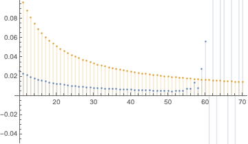
Refer to caption
Figure 10: Numerical evaluation of the upper bound (orange curve) and of the exact Wasserstein distance in (blue curve) for n∈{10,70}n\in\left\{10,70\right\}. The numerical evaluation of the Wasserstein distance becomes unstable for n≥50n\geq 50.
Example D.2 (Binomial vs Hypergeometric).

If Xn∼Hyper​(n,K,N)X_{n}\sim\mbox{Hyper}(n,K,N) and X∞∼Bin​(n,K/N)X_{\infty}\sim\mbox{Bin}(n,K/N), then a direct application of classical Stein’s method gives the bound (n−1)/(N−1)(n-1)/(N-1) already provided in [18, 29]. Equation (3.10) gives

T​V​(Bin​(n,K/N),Hyper​(n,K,N))\displaystyle TV(\mbox{Bin}(n,K/N),\mbox{Hyper}(n,K,N)) ≤I​EH​[|(n−X)​(K⁡(n−1)−N​X)(N−K)​(K+n−N−X−1)​(1+X)|​PB​(X)​(1−PB​(X))pB​(X+1)]\displaystyle\leq{\rm I\kern-1.60004ptE}_{H}\left[\left|\frac{(n-X)(K(n-1)-NX)}{(N-K)(K+n-N-X-1)(1+X)}\right|\frac{P_{B}(X)(1-P_{B}(X))}{p_{B}(X+1)}\right]

where the index HH denote the expectation computed for the hypergeometric distribution and the index BB is associated to the binomial distribution. The bound is not as readable as [17], who obtain the incredibly elegant 1−(1−1/N)n−11-(1-1/N)^{n-1}. If we choose the Hypergeometric as target distribution, we obtain

T​V​(Bin​(n,K/N),Hyper​(n,K,N))\displaystyle TV(\mbox{Bin}(n,K/N),\mbox{Hyper}(n,K,N)) ≤I​EB​[|(n−X)​(K⁡(n−1)−N​X)(N−K)​(K+n−N−X−1)​(1+X)|​PH​(X)​(1−PH​(X))pH​(X+1)].\displaystyle\leq{\rm I\kern-1.60004ptE}_{B}\left[\left|\frac{(n-X)(K(n-1)-NX)}{(N-K)(K+n-N-X-1)(1+X)}\right|\frac{P_{H}(X)(1-P_{H}(X))}{p_{H}(X+1)}\right].

The three bounds are graphically compared in Figure 11.

Refer to caption
Figure 11: Bounds for the total variation distance between the binomial (n,K/N)(n,K/N) and the hypergeometric (n,K,N)(n,K,N) for K=20K=20 and N=50N=50. The blue and orange curve correspond to our bounds, and the green one is that from [17].

We conclude with two examples which are outside the scope of our Corollaries 3.4 and B.2. To prepare for these, we make some simplifying assumptions. We suppose that p∞p_{\infty} is continuous (ℓ=0\ell=0) with support either the half line (00 may or may not be included) or the real line. Let 𝒯∞\mathcal{T}_{\infty} and ℒ∞\mathcal{L}_{\infty} be its Stein operators and set gh​(x)=ℒ∞​h​(x)c⁡(x)g_{h}(x)=\frac{\mathcal{L}_{\infty}h(x)}{c(x)}. Next let XnX_{n} have operators 𝒯nℓ\mathcal{T}_{n}^{\ell} and ℒnℓ\mathcal{L}_{n}^{\ell} (ℓ∈{−1,0,1}\ell\in\left\{-1,0,1\right\}) and suppose that 𝒮⁡(pn)\mathcal{S}(p_{n}) has infimum (minimum) an≥0a_{n}\geq 0 and supremum (maximum) bn≤∞b_{n}\leq\infty. Starting again from (3.4), we know that for all sufficiently regular functions cc we can write

𝔼​h​(Xn)−𝔼​h​(X∞)=𝔼⁡[𝒯∞​c​(Xn)​gh​(Xn)+c⁡(Xn)​gh′​(Xn)]\displaystyle\mathbb{E}h(X_{n})-\mathbb{E}h(X_{\infty})=\mathbb{E}\left[\mathcal{T}_{\infty}c(X_{n})g_{h}(X_{n})+c(X_{n})g_{h}^{\prime}(X_{n})\right]
=𝔼⁡[(𝒯∞​c​(Xn)−𝒯nℓ​c​(Xn))​gh​(Xn)]+𝔼⁡[c⁡(Xn)​(gh′​(Xn)−Δ−ℓ​gh​(Xn))]−κnℓ​(h)\displaystyle=\mathbb{E}\left[(\mathcal{T}_{\infty}c(X_{n})-\mathcal{T}_{n}^{\ell}c(X_{n}))g_{h}(X_{n})\right]+\mathbb{E}\left[c(X_{n})\left(g_{h}^{\prime}(X_{n})-\Delta^{-\ell}g_{h}(X_{n})\right)\right]-\kappa_{n}^{\ell}(h) (D.1)

where

κnℓ(h)={−c(an)/c(an−1)pn(an)ℒ∞h(an−1) if ​ℓ=1limx→bnℒ∞​h​(x)​pn​(x)−limx→anℒ∞​h​(x)​pn​(x) if ℓ=0c⁡(bn)/c⁡(bn−1)​pn​(bn)​ℒ∞​h​(bn) if ℓ=−1.\displaystyle\kappa_{n}^{\ell}(h)=\begin{cases}-c(a_{n})/c(a_{n}-1)p_{n}(a_{n})\mathcal{L}_{\infty}h(a_{n}-1)&\mbox{ if }\ell=1\\ \lim_{x\to b_{n}}\mathcal{L}_{\infty}h(x)p_{n}(x)-\lim_{x\to a_{n}}\mathcal{L}_{\infty}h(x)p_{n}(x)&\mbox{ if }\ell=0\\ c(b_{n})/c(b_{n}-1)p_{n}(b_{n})\mathcal{L}_{\infty}h(b_{n})&\mbox{ if }\ell=-1.\end{cases}

Controlling ghg_{h} and gh′g_{h}^{\prime} via the results from Sections 2.2 and 2.3 easily leads to bounds on the usual probability metrics.

Example D.3 (Maxima of independent to Fréchet).

Let the target p∞p_{\infty} be the Fréchet distribution studied in Example C.4 and suppose that XnX_{n} has continuous distribution (i.e. ℓ=0\ell=0). Then taking c⁡(x)=xα+1c(x)=x^{\alpha+1} we have 𝒯∞​c​(x)=α\mathcal{T}_{\infty}c(x)=\alpha so that (D.1) yields

|𝔼​h​(Xn)−𝔼​h​(X∞)|\displaystyle\left|\mathbb{E}h(X_{n})-\mathbb{E}h(X_{\infty})\right| =|𝔼⁡[(α−𝒯n​c1​(Xn))​gh​(Xn)]−κnℓ​(h)|\displaystyle=\left|\mathbb{E}\left[(\alpha-\mathcal{T}_{n}c_{1}(X_{n}))g_{h}(X_{n})\right]-\kappa_{n}^{\ell}(h)\right|
≤𝔼⁡[|α−𝒯n​c1​(Xn)|​1−e−Xn−αα]+|κnℓ​(h)|\displaystyle\leq\mathbb{E}\left[\left|\alpha-\mathcal{T}_{n}c_{1}(X_{n})\right|\frac{1-e^{-X_{n}^{-\alpha}}}{\alpha}\right]+\left|\kappa_{n}^{\ell}(h)\right|
≤𝔼⁡[|1−1α​𝒯n​c1​(Xn)|]−κnℓ​(h)\displaystyle\leq\mathbb{E}\left[\left|1-\frac{1}{\alpha}\mathcal{T}_{n}c_{1}(X_{n})\right|\right]-\kappa_{n}^{\ell}(h)

for all hh such that κ1≤1\kappa_{1}\leq 1, and therefore also for the Kolmogorov distance. Now suppose that Mn=max⁡(X1,…,Xn)M_{n}=\max(X_{1},\ldots,X_{n}) the maximum of nn independent positive random variables with pdf f⁡(x)f(x), cdf F⁡(x)F(x) and support [a,b][a,b]. Set Xn=Mn/rnX_{n}=M_{n}/r_{n} for rnr_{n} some sequence of normalizing constants. Then an=a/rna_{n}=a/r_{n}, bn=b/rnb_{n}=b/r_{n}, Pn​(x)=F​(rn​x)nP_{n}(x)=F({r_{n}}x)^{n} and pn​(x)=n​rn​f​(rn​x)​F​(rn​x)n−1p_{n}(x)=n{r_{n}}f({r_{n}}x)F({r_{n}}x)^{n-1} so that

𝒯n​c1​(x)=(α+1)​xα+rn​xα+1​(f′​(rn​x)f⁡(rn​x)+(n−1)​f⁡(rn​x)OPENF​r​an​x))\displaystyle\mathcal{T}_{n}c_{1}(x)=(\alpha+1)x^{\alpha}+r_{n}x^{\alpha+1}\left(\frac{f^{\prime}(r_{n}x)}{f(r_{n}x)}+(n-1)\frac{f(r_{n}x)}{Fra_{n}x)}\right)

for a/rn≤x≤b/rna/r_{n}\leq x\leq b/r_{n}. Also κnℓ​(h)=ℒ∞​h​(b−/rn)​n​rn​f​(b−)​F​(b−)n−1−ℒ∞​h​(a+/rn)​n​rn​f​(a+)​F​(a+)n−1\kappa_{n}^{\ell}(h)=\mathcal{L}_{\infty}h(b^{-}/r_{n})nr_{n}f(b^{-})F(b^{-})^{n-1}-\mathcal{L}_{\infty}h(a^{+}/r_{n})nr_{n}f(a^{+})F(a^{+})^{n-1}. If, for instance, we choose F(x)=(1−x−α)𝕀[x≥1]F(x)=(1-x^{-\alpha})\mathbb{I}[x\geq 1] the Pareto distribution with rn=n1/αr_{n}=n^{1/\alpha} then a=1a=1, an=n−1/αa_{n}=n^{-1/\alpha}, b=bn=∞b=b_{n}=\infty, and pn​(x)=α​x−α−1​(1−x−α/n)n−1p_{n}(x)=\alpha x^{-\alpha-1}(1-x^{-\alpha}/n)^{n-1} for x≥n−1/αx\geq n^{-1/\alpha} so that κnℓ​(h)=0\kappa_{n}^{\ell}(h)=0 and 1α​𝒯n​c1​(x)=n−1n​(1−x−αn)−1,\frac{1}{\alpha}\mathcal{T}_{n}c_{1}(x)=\frac{n-1}{n}\big(1-\frac{x^{-\alpha}}{n}\big)^{-1}, x≥n−1/α.x\geq n^{-1/\alpha}. We readily obtain

𝔼⁡[|1−1α​𝒯n​c1​(Xn)|]=𝔼⁡[|1−n−1n​(1−Xn−αn)−1|]=2n−1​(1−1n)n≤2/en−1\mathbb{E}\left[\left|1-\frac{1}{\alpha}\mathcal{T}_{n}c_{1}(X_{n})\right|\right]=\mathbb{E}\left[\left|1-\frac{n-1}{n}\left(1-\frac{X_{n}^{-\alpha}}{n}\right)^{-1}\right|\right]=\frac{2}{n-1}\left(1-\frac{1}{n}\right)^{n}\leq\frac{2/e}{n-1}

independently of α\alpha. See also [31, Section 2.6].

Example D.4 (Binomial to normal).

Consider p∞p_{\infty} the standard normal density, and pnp_{n} the density of XnX_{n} a standardized binomial with parameters n,θn,\theta, that is Xn=(Bn−n​θ)/n​θ​(1−θ)X_{n}=(B_{n}-n\theta)/\sqrt{n\theta(1-\theta)} where Bn∼Bin⁡(n,θ)B_{n}\sim\mathrm{Bin}(n,\theta). Let rn=n​θ​(1−θ)r_{n}=\sqrt{n\theta(1-\theta)}. Then an=−nθ/rna_{n}=-n\theta/r_{n} and bn=n⁡(1−θ)/rnb_{n}=n(1-\theta)/r_{n} and

pn(x)=(nn​θ+rn​x)θn​θ+rn​x(1−θ)n⁡(1−θ)−rn​x for x∈𝒮(pn)={k−n​θrn with k∈{0,…,n}}.p_{n}(x)=\binom{n}{n\theta+r_{n}x}\theta^{n\theta+r_{n}x}(1-\theta)^{n(1-\theta)-r_{n}x}\mbox{ for }x\in\mathcal{S}(p_{n})=\left\{\frac{k-n\theta}{r_{n}}\mbox{ with }k\in\left\{0,\ldots,n\right\}\right\}.

An appropriate derivative in this case is Δnℓ​f​(x)=rn/ℓ⁡(f⁡(x+ℓ/rn)−f⁡(x))\Delta^{\ell}_{n}f(x)=r_{n}/\ell(f(x+\ell/r_{n})-f(x)), ℓ∈{−1,1}\ell\in\left\{-1,1\right\}; note that if ff is twice differentiable then, from Taylor’s theorem

Δnℓ​f​(x)=f′​(x)+1rn​𝔼​[V​f′′​(X+U​Vrn)]\displaystyle\Delta^{\ell}_{n}f(x)=f^{\prime}(x)+\frac{1}{r_{n}}\mathbb{E}\Big[Vf^{\prime\prime}\Big(X+\frac{UV}{r_{n}}\Big)\Big]

where U,VU,V are independent uniform on [0,1][0,1]. The canonical operator for pnp_{n} is

𝒯nℓ​f​(x)\displaystyle\mathcal{T}_{n}^{\ell}f(x) =Δnℓ​(f⁡(x)​pn​(x))pn​(x)\displaystyle=\frac{\Delta^{\ell}_{n}(f(x)p_{n}(x))}{p_{n}(x)}
=rn(f(x+1rn)θ1−θn⁡(1−θ)−x​rnn​θ+1+x​rn−f(x))(ℓ=1)\displaystyle=r_{n}\left(f\left(x+\frac{1}{r_{n}}\right)\frac{\theta}{1-\theta}\frac{n(1-\theta)-xr_{n}}{n\theta+1+xr_{n}}-f(x)\right)\qquad(\ell=1)
=rn(f(x)−f(x−1rn)1−θθn​θ+x​rnn⁡(1−θ)+1−x​rn)(ℓ=−1)\displaystyle=r_{n}\left(f(x)-f\left(x-\frac{1}{r_{n}}\right)\frac{1-\theta}{\theta}\frac{n\theta+xr_{n}}{n(1-\theta)+1-xr_{n}}\right)\qquad(\ell=-1)

for x∈𝒮⁡(pn)x\in\mathcal{S}(p_{n}) and pnp_{n} satisfies the identities

𝔼⁡[𝒯nℓ​c​(Xn)​f​(Xn)+c⁡(Xn)​Δn−ℓ​f​(Xn)]=κnℓ​(c,f)\displaystyle\mathbb{E}[\mathcal{T}_{n}^{\ell}c(X_{n})f(X_{n})+c(X_{n})\Delta^{-\ell}_{n}f(X_{n})]=\kappa_{n}^{\ell}(c,f)

with κn+(c,f)=−c(−nθ/rn)f((−nθ−1)/rn)pn(−nθ/rn)\kappa_{n}^{+}(c,f)=-c(-n\theta/r_{n})f((-n\theta-1)/r_{n})p_{n}(-n\theta/r_{n}) and κn−​(c,f)=c⁡(n⁡(1−θ)/rn)​f​(((n⁡(1−θ)+1)/rn)​pn​(n⁡(1−θ)/rn)𝐶𝐿𝑂𝑆𝐸\kappa_{n}^{-}(c,f)=c(n(1-\theta)/r_{n})f(((n(1-\theta)+1)/r_{n})p_{n}(n(1-\theta)/r_{n}). If we pick c⁡(x)=1c(x)=1 then, after some simplifications,

𝒯∞​c​(x)−𝒯n+​c​(x)\displaystyle\mathcal{T}_{\infty}c(x)-\mathcal{T}_{n}^{+}c(x) =−x−rn​(rn2−x​rn​θrn2+x​rn​(1−θ)+(1−θ)−1)\displaystyle=-x-r_{n}\left(\frac{r_{n}^{2}-xr_{n}\theta}{r_{n}^{2}+xr_{n}(1-\theta)+(1-\theta)}-1\right)
=−x+rn​(x​rn−(1−θ)rn2+x​rn​(1−θ)+(1−θ))\displaystyle=-x+r_{n}\left(\frac{xr_{n}-(1-\theta)}{r_{n}^{2}+xr_{n}(1-\theta)+(1-\theta)}\right)
=−x+x⁡(rn2−(1−θ)​rn/xrn2+x​rn​(1−θ)+(1−θ))\displaystyle=-x+x\left(\frac{r_{n}^{2}-(1-\theta)r_{n}/x}{r_{n}^{2}+xr_{n}(1-\theta)+(1-\theta)}\right)
=−(1−θ)​(x2+1)​rn+xrn2+x​rn​(1−θ)+(1−θ).\displaystyle=-(1-\theta)\frac{(x^{2}+1)r_{n}+x}{r_{n}^{2}+xr_{n}(1-\theta)+(1-\theta)}.

This function is negative throughout 𝒮⁡(pn)\mathcal{S}(p_{n}) and explicit computations (we use Mathematica) inform us that

𝔼⁡[|𝒯∞​c​(x)−𝒯n+​c​(x)|]≤2​1θ−1​1n\displaystyle\mathbb{E}\left[\left|\mathcal{T}_{\infty}c(x)-\mathcal{T}_{n}^{+}c(x)\right|\right]\leq 2\sqrt{\frac{1}{\theta}-1}\frac{1}{\sqrt{n}}

(the exact expression is not very enlightening). With obvious accommodations to the notations, we have κn+(h)=(1−θ)nℒ∞h(−nθ/rn)\kappa_{n}^{+}(h)=(1-\theta)^{n}\mathcal{L}_{\infty}h(-n\theta/r_{n}). For the sake of brevity we only consider the case of Wasserstein distance with h⁡(x)h(x) Lipschitz. Then |gh​(x)|≤1|g_{h}(x)|\leq 1 and |gh′′​(x)|≤2|g_{h}^{\prime\prime}(x)|\leq 2 (this result is available e.g. from [11, Lemma 2.4]) so that

Wass⁡(pn,p∞)≤2​1θ−1​1n+2n​θ​(1−θ)+(1−θ)n.\displaystyle\mathrm{Wass}(p_{n},p_{\infty})\leq 2\sqrt{\frac{1}{\theta}-1}\frac{1}{\sqrt{n}}+\frac{2}{\sqrt{n\theta(1-\theta)}}+(1-\theta)^{n}.

We could also obtain rates in the Kolmogorov and Total Variation distances, but this would require more work for what is, ultimately, only a proof of concept. As far as we are aware, the first to have performed Stein’s method of comparison of generators for comparing a discrete and a continuous distribution are [28].

(M. Ernst) Département de Mathématique, Faculté des Sciences, Université de Liège, Belgium

(Y. Swan) Département de Mathématique, Faculté des Sciences, Université libre de Bruxelles, Belgium

E-mail address, M. Ernst m.ernst@uliege.be

E-mail address, Y. Swan yvswan@ulb.ac.be