On Locally Decodable Codes in Resource Bounded Channels
Abstract
Constructions of locally decodable codes (s) have one of two undesirable properties: low rate or high locality (polynomial in the length of the message). In settings where the encoder/decoder have already exchanged cryptographic keys and the channel is a probabilistic polynomial time (PPT) algorithm, it is possible to circumvent these barriers and design s with constant rate and small locality. However, the assumption that the encoder/decoder have exchanged cryptographic keys is often prohibitive. We thus consider the problem of designing explicit and efficient s in settings where the channel is slightly more constrained than the encoder/decoder with respect to some resource e.g., space or (sequential) time. Given an explicit function that the channel cannot compute, we show how the encoder can transmit a random secret key to the local decoder using and a random oracle . We then bootstrap the private key construction of Ostrovsky, Pandey and Sahai (ICALP, 2007), thereby answering an open question posed by Guruswami and Smith (FOCS 2010) of whether such bootstrapping techniques are applicable to s in channel models weaker than just PPT algorithms. Specifically, in the random oracle model we show how to construct explicit constant rate s with locality of in the security parameter against various resource constrained channels.
1 Introduction
Consider the classical one-way communication setting where two parties, the sender and receiver, communicate over a noisy channel that may corrupt parts of any message sent over it. An error correcting code is an invertible transformation mapping messages into codewords that are then transmitted over the noisy channel. The goal is to ensure that the decoder can (w.h.p.) reliably recover the entire message from the corrupted codeword. For locally decodable codes (s) we have an even stronger goal: The decoder should be able to reliably recover any individual bit of the original message (w.h.p.) by examining at most bits of the corrupted codeword. An ideal should have a good rate (i.e., the codeword should not be much longer than the original message) and small locality .
Historically, there have been two major lines of work associated with modelling the channel behavior. In Shannon’s symmetric channel model, the channel corrupts each bit of the codeword independently at random with some fixed probability. By contrast, in Hamming’s adversarial channel model the channel corrupts the codeword in a worst case manner subject to an upper bound on the total number of corruptions.
Unsurprisingly, when we work in Shannon’s channel model it is much easier to design s with good rate/locality. By contrast, state of the art constructions for Hamming channels either have very high locality e.g., [KMRS17] or poor rate e.g., Hadamard codes have constant locality but the codeword has exponential length. Unfortunately, in many real-world settings independent random noise is not a realistic model of channel behavior e.g., burst-errors are common in reality, but unlikely in Shannon’s model. Thus, coding schemes designed to work in Shannon’s channel model are not necessarily suitable in practice. By contrast, coding schemes designed to work in Hamming’s adversarial setting must be able to handle any error pattern.
Our central motivating goal is to find classes of adversarial channels that are expressive enough to model any error patterns that would arise in nature, yet admit s with good decoding algorithms. s have found remarkable applications throughout various fields, notably private information retrieval schemes [BI01, CKGS98, KO97], psuedo-random generator constructions [BFNW91, STV01], self-correcting computations [DJK+02, GLR+91], PCP systems [BFALS91] and fault tolerant storage systems [KT00].
Lipton [Lip94] introduced the adversarial computationally bounded model, where the channel was viewed as a Hamming channel restricted to bounded corruption by a probabilistic polynomial time (PPT) algorithm. The notion of adversaries being computationally bounded is well-motivated by real-world channels that have some sort of limitations on their computations i.e., we expect error patterns encountered in nature to be modeled by some (possibly unknown) PPT algorithm. We argue that even Lipton’s channel significantly overestimates the capability of the channel. For example, if the channel has reasonably small latency, say seconds, and the world’s fastest single core processor can evaluate 10 billion instructions per second then the depth of any (parallel) computation performed by the channel is at most billion operations.
This view of modelling the channel as more restricted than just PPT was further explored by Guruswami and Smith [GS16] who studied channels that could be described by simple (low-depth) circuits. Remarkably, even such a simple restriction allowed them to design codes that enjoyed no public/private key setup assumptions, while matching the Shannon capacity using polynomial time encoding/decoding algorithms. With such positive results, it is natural to ask whether similar results may be expected for s.
1.1 Contributions
We introduce resource bounded adversarial channel models which admit s with good locality whilst still being expressive enough to plausibly capture any error pattern for most real-world channels. We argue that these resource bounded channel models are already sufficiently expressive to model any corruption pattern that might occur in nature e.g., burst-errors, correlated errors. For example, observe that the channel must compute the entire error pattern before the codeword is delivered to the receiver. Thus, the channel can be viewed as sequentially time bounded e.g., the channel may perform arbitrary computation in parallel but the total depth of computation is bounded by the latency of the channel. The notion of a space bound (or space-time bound) channel can be similarly motivated.
We introduce safe functions as a general way to characterize friendly channels. Intuitively, a function is “safe” for a class of channels if the channel is not able to predict given . We show how to construct safe functions for several classes of resource bounded channels including time bounded, space bounded, and cumulative memory cost bounded channels in the parallel random oracle model. For example, in the random oracle model the function is a safe function for the class of sequentially time-bounded adversaries i.e., it is not possible to evaluate the function using fewer than sequential calls to the random oracle . We also discuss how to construct safe functions for the class of space (resp. space-time) bounded channels using random oracles.
Furthermore, we give a general framework for designing good locally decodable codes against resource bounded adversarial channels by using safe functions to bootstrap existing private-key constructions. Our framework assumes no a priori private or public key setup assumptions, and constructs explicit s over the binary alphabet11 1 Note that small alphabet sizes are attractive for practical channels designed to transmit bits efficiently. with constant rate against any class of resource bounded adversaries admitting safe functions.
Our local decoder can decode correctly with arbitrarily high constant probability after examining at most bits of the corrupted codeword, where is the security parameter22 2 In this paper we use the security parameter in an asymptotic sense e.g., for any attacker running in time there is a negligible function upper bounding the probability that the attacker succeeds. In particular, the function is negligible, but does not provide -bits of concrete security i.e., any attacker running in time succeeds with probability at most . and is any function such that e.g., or . By contrast, state of the art constructions for Hamming channels have very high locality e.g., [KMRS17]. Our codes are robust against a constant fraction of corruptions, and are (essentially) non-adaptive i.e., the local decoding algorithm can decode after submitting just two batches of queries.
Our constructions stand at the intersection of coding theory and cryptography, using well-known tools and techniques from cryptography to provide notions of (information theoretic) randomness and security for communication protocols between sender/receiver. To prove the security of our constructions, we introduce a two-phase distinguisher hybrid argument, which may be of independent interest for other coding theoretic problems in these resource bounded channel models.
1.2 Technical Overview
Private s.
Our starting point is the private locally decodable codes of [OPS07]. These s permit nearly optimal query complexity, asymptotically positive rate and reliable decoding with high probability, but make the strong assumption that the sender and receiver have already exchanged a secret key that is unknown to the PPT adversarial channel over which they communicate. In our setting the sender and the receiver do not have access to any secret key. Our constructions thus reduce the general setting (no setup assumptions) against resource bounded channels to the shared private key setting against these channels, so that we can bootstrap private constructions.
Bootstrapped Encoder/Decoder.
Our encoder uses the following high level template: (1) samples a random seed (2) computes a predetermined safe function on the seed and extracts a secret key from (e.g., using a random oracle) (3) Uses the private encoder to encode the message using (4) appends a reliable encoding (repetition code) of the random seed to the codeword. The local decoder (1) decodes the random seed (random sampling + majority vote). (2) Evaluates the safe function to recover the secret key . (3) Uses the private decoder with the secret key to recover the desired bit of the original message.
Security Proof.
We remark that there are a few subtle challenges that arise when we prove that our bootstrapped construction is secure. We want to prove that the channel will (w.h.p.) fail to produce a corrupted codeword that fools the local decoding algorithm. Towards this goal we might try to prove that the channel cannot distinguish the derived key from a truly random key even given the nonce . However, this is insufficient to prove that the local decoder is successful because the local decoder is able to recover from . We introduce a novel two-phase distinguisher game to address these challenges. In particular, we consider an attacker-distinguisher pair who tries to predict whether or not the secret encoding key is derived from the nonce or was selected uniformly at random . In phase 1 the (resource bounded) attacker generates a corrupted codeword which is given to the distinguisher in phase 2 who must then guess whether or . The distinguisher is computationally unbounded, but is not allowed to query the random oracle. If is a safe function then the advantage of any such attacker-distinguisher pair can be shown to be negligible. We demonstrate that any channel which succeeds at fooling our local decoder yields an attacker-distinguisher pair for this two phase game — the distinguisher works by simulating the private decoder to distinguish between the two aforementioned encodings. It follows that the channel cannot fool the local decoder (except with negligible probability).
1.3 Related Work
Many existing code constructions consider an underlying channel that can only introduce a bounded number of errors, but has an unlimited time to adversarially decide the positions of these errors. These codes are therefore resilient to any possible error pattern with a bounded number of corruptions, corresponding to Hamming’s error model, and are safe for data transmission. However, this resiliency to the worst-case error leads to coding limitations and some possibly undesirable tradeoffs. On one hand, current constructions for s that focus on efficient encoding can obtain any constant rate while simultaneously being robust to any constant fraction of errors and using queries for decoding [KMRS17]. On the other hand, codes that focus on low query complexity obtain blocklength that is subexponential in the message length while using a constant number of queries [Yek08, Efr12, DGY11]. Finally, if exactly queries are desired, any code must use blocklength exponential in the message length [KdW04]. Avoiding such drastic tradeoffs between blocklength and query complexity would be attractive for other natural channels in contrast to Hamming’s error model. For example, Shannon introduces a model in which each symbol has some independent probability of being corrupted; this probability is generally fixed across all symbols and known a priori. However, this probabilistic channel may be too weak to capture natural phenomenon such as bursts of consecutive error.
Thus it is reasonable to believe that many natural channels lie between these two extremes; in particular, Lipton [Lip94] argues that many reasonable channels are computationally bounded and can be modeled as PPT algorithms. In this model, [Lip94] introduced an analog to classical error-correcting codes that is robust to a fraction of errors beyond the rates provably tolerable by any code in the adversarial Hamming channel model. Similarly, a line of work [Lip94, MPSW05, GS16, SS16] have improved upon the error rate limits of classical error-correcting codes in slight variants of Lipton’s computationally bounded channel model. A weakness of the codes introduced by [Lip94] is the strong cryptographic assumption that the sender and receiver share a secret random string unknown to the channel. This weakness is ameliorated by [MPSW05], who observe that if a message is encoded by digitally signing a code that is list-decodable with a secret key, then an adversarial PPT is unlikely to produce valid signatures. Conversely, the decoder can select the unique message from the list of possible messages with a valid signature, effectively producing public-key error-correcting codes against computationally bounded channels. Subsequently, [GS16] further removes the public-key setup assumption specifically for the channel in which either the error is independent of the actual message being sent, or the errors can be described by polynomial size circuits. Their results are based on the idea that the sender can choose a permutation and some key that is computable by the decoder but not by the channel, since it operates with low complexity. In some loose sense, their results are an example of our framework when the channel has bounded circuit complexity, i.e. the bounded resource is circuit complexity of the error.
[OPS07] obtain s with constant information and error rates over the binary alphabet against computationally bounded errors, using a small number of queries to the corrupted word; specifically they can achieve any query complexity, where is the desired security parameter. However, their results not only assume the existence of one-way functions, but also once again assume a predetermined private key known to both the encoder and decoder but not the channel, similar to [Lip94]. Analogous to the improvements of [MPSW05] for classical error codes, [HO08, HOSW11] construct public-key s, assuming the existence of -hiding schemes [CMS99] and IND-CPA secure cryptosystems.
Ben-Sasson et al. [BGH+06] introduce the concept of relaxed locally decodable codes (s) as an alternative means of decreasing the tradeoffs between rate and locality in classical s. In contrast to s, the decoding algorithm for s is allowed to output sometimes to reveal that the correct value is unknown, though it is limited in the fraction of outputs in which it can output . The s proposed by Ben-Sasson et al. [BGH+06] obtain constant query complexity and blocklength . Subsequently, Gur et al. [GRR18] construct relaxed locally correctable codes (s) with attractive properties but significant tradeoffs; they propose codes with constant query complexity and error rate but block length roughly quartic in the message length as well as codes with constant error rate and linear block length, but quasipolynomial () query complexity. These parameters are significantly better than classical locally correctable codes and their results immediately extend to s, since the original message is embedded within the initial part of the encoding. However, these tradeoffs are still undesirable.
Recently, Blocki et al. [BGGZ19] study s and s on adversarial but computationally bounded channels in an effort to reduce these tradeoffs. They obtain s and s over the binary alphabet, with constant information rate, and poly-logarithmic locality. Moreover, their codes require no public-key or private-key cryptographic setup; the only setup assumption required is the selection of the public parameters (seed) for a collision-resistant hash function.
2 Preliminaries
2.1 Notation
We use the notation to represent the set . For any , let denote the Hamming weight of , i.e. the number of non-zero coordinates of . Let denote the Hamming distance between the vectors and . All logarithms will be base . For vectors , we use to denote the vector that appears most frequently. If such a vector is not unique, then an arbitrary vector of highest frequency is chosen. For any vector , let be the coordinate of . We also let denote the concatenation of with and denote the bitwise XOR of and . For a randomized function , the notation will be used to denote that uses random coins as its randomness. A function is said to be negligible in if for any non-zero polynomial . Finally, we distinguish between inputs and parameters to a function as follows: .
2.2 Locally Decodable Codes
We consider the setting where sender encodes a message into a codeword using an encoding algorithm so that is sent over noisy channel , which then hands over the possibly corrupted codeword to , who then uses a decoding algorithm to obtain the original message. We denote and where is the alphabet. We denote the alphabet size by . We consider the model where corresponds to with some symbols replaced with others in . The term corruptions refers to such symbol replacements within , with a single corruption meaning a single symbol replacement, so that . The encoding and decoding algorithms are denoted by and . We use the terms sender, encoder, and encoding algorithm interchangeably, and similarly for receiver, decoder, and decoding algorithm.
A code is an encoder-decoder pair. The information rate or simply rate of the code is the ratio , so that a lower rate corresponds to a larger amount of information redundancy introduced by the code. The message length, codeword length, and alphabet size characterize a coding scheme. Coding schemes with high rate and low alphabet size are desired.
An error correcting code allows the decoder to recover the entire original message by reading the entire . It is also possible to construct codes that only need to read a few symbols of rather than the entire message to recover a small part of the message. Such codes are called locally decodable codes (), and will be the focus of this work. An has locality , error rate and error correction probability if any character of may be recovered with probability at least by making at most queries to , even when the channel corrupts fraction of all symbols of to generate . We use the terms query complexity and locality interchangeably. When and are clear from context (as constants), the scheme may be referred to as an - . Naturally, s with low locality, high error rate, and high error correction probability are desired.
2.3 Definitions
The focus of this work will be the construction of s (Section 2.4) for resource-bounded channels (Section 4.1). In this section, we present several building blocks that we will require in our constructions — , private-s and safe functions. We first give two classical definitions pertaining to s that compactly summarize our discussion in Section 2.2.
Definition 1.
A -coding scheme is a pair of encoding and decoding algorithms where . The information rate of the scheme is defined as .
Definition 2.
A -coding scheme is an -locally decodable code () if , with query access to a word such that , on input index , makes at most queries to and outputs with probability at least over the randomness of the decoder.
Next, we present a simple variant of s which we denote by . These will be very similar to s except that they are required to decode the entire original message while making as few queries to the corrupted codeword as possible. They are defined with respect to the same setting as in Section 2.2.
Definition 3.
A -coding scheme is an - if , with query access to a word such that , makes at most queries to and outputs with probability at least over the randomness of the decoder.
We remark that it will be typically desired that for an , the locality be even when is very large. We now move on to define private-s analogous to Definition 2 as an alternative to that given by [OPS07] – refer to Appendix D for an overview of [OPS07].
Definition 4.
(One-Time Private Key LDC) A triplet of probabilistic algorithms is an -private locally decodable code (private ) against a class if makes at most queries and for all attackers and all messages we have
where the probability is taken over all the random coins of and . If is the set of all (computationally unbounded) attackers we simply say that the scheme is a -private LDC.
Our contributions in the subsequent sections will assume that the coding scheme and channel all have access to a random oracle. Furthermore, we assume that the channel is a pROM algorithm with respect to this random oracle (refer to the initial discussion in Section 4.1 for an overview of the pROM model). The following definition establishes a notion of privacy against classes (i.e. sets) of adversarial channels in terms of “hard to compute” functions.
Definition 5 (Safe Function).
We say that a function is -safe for a class of algorithms if for all we have
where the probability is taken over the random coins of and the selection of an input . If the function is defined using a random oracle, then the probability is also taken over the selection of the random oracle .
We will use the notation to denote a safe function for class . In the above definition, we usually think of as being a negligibly small parameter. We remark that in the parallel random oracle model, one can construct functions with sharp thresholds on the required resources. For example, the function is trivial to compute using at most sequential queries to , but any parallel algorithm making at most queries over rounds succeeds with probability at most .
Precomputation.
Definition 5 can be extended to consider an attacker who is allowed to perform precomputation with the random oracle before receiving the input . In particular, we could consider a pair of oracle algorithms where outputs an -bit hint for after making at most queries to . We could modify the definition to require that for all we have
where the randomness is taken over the selection of , the random oracle , and the random coins of . Here, (precomputation) is not necessarily constrained to be in the same class as .
We remark that for , a precomputing attacker can succeed with probability at least by having output the hint . Then first checks if and, if so, simply returns the output which is already recorded in the hint . Thus, we need the length of the random nonce to be sufficiently large to resist brute-force precomputation attacks. By contrast, if the attacker does not get to perform any precomputation then can be negligible even when .
All of the safe functions we consider would also be secure under this stronger notion. For example, is -safe for where is a random bit string, makes at most total random oracle queries, and makes at most total queries in at most rounds to . In our constructions we select a random nonce of length to ensure that a precomputing attacker fails.
2.4 Our Model
We first define an experiment to model the interaction between a code and an algorithm from a class of pROM algorithms adversarial against the code. For random oracle , let be a -coding scheme in the random oracle model and let be a class of pROM algorithms. Then, the interaction of having error rate , with the code is defined in Figure 2 (analogous to priv-LDC-Sec-Game defined in Figure 1). Here, the security parameter , and the decoding probability are also given as inputs to the game. We now formally define a notion of s analogous to Definition 2, but with respect to general classes of adversarial (pROM) channels.
Definition 6.
Let be a class of pROM algorithms. A -coding scheme is an -locally decodable code () if makes at most queries and for all and all messages we have
where the probability is taken over the random coins of and the selection of the random oracle .
We remark that our codes need not require that each message have the same length. Jumping slightly ahead, longer messages only need proportionally longer repetition codes to guarantee transmittance of the secret key. However for the sake of presentation, we use notation for fixed length messages.
3 Constructions
We begin by discussing the use of safe functions in Section 3.1 and give several examples of constructing such functions in Section 4. We then show how allowing an encoder/decoder pair with enough resources to compute safe functions can effectively generate a random shared secret key between the pair. This secret key can then be bootstrapped into existing private constructions to give codes against resource bounded adversaries. We give our final framework in Section 3.2 and the main proofs in Sections 3.3 and 3.4.
3.1 Using Safe Functions
Let be a class of algorithms with safe function . For some input to , we will be interested in bounding the probability of the undesirable event where the queries the random oracle at any string of the form with . In the absence of such an event, would information theoretically appear random to . Lemma 1 shows that such an event may only happen with negligible probability where is the total number of random oracle queries.
Lemma 1.
For a some class of pROM algorithms with safe function , let be the event that on some input , queries the random oracle at for any . Then , where is the number of oracle queries made by .
Proof.
We prove the claim by a reduction argument. By way of contradiction, suppose there exists a such that on input string , makes queries to the random oracle and . We construct an adversary as follows: on input , the adversary
- •
Simulates with input
- •
Keeps track of all queries by which queries the random oracle
- •
On termination of , returns the suffix of length |(x)| from one of the queries selected uniformly at random
However, we know that queries the random oracle at with probability . Since picks one of ’s queries at random, , which contradicts the definition of safe function. ∎
Assuming that never queries the random oracle at any point of the form with (for some ) we can view each as a fresh -bit string. Thus, we can obtain a random -bit string by concatenating all of the labels for each . This motivates the following definition of an expansion family which will be used in subsequent sections.
Definition 7 (Expansion Family).
For random oracle the expansion family of functions where each function is defined as , where the prefix of for each oracle query in the definition is expressed in binary using bits.
3.2 Framework for s against Resource Bounded Channels
Our aim in this section will be to achieve s having no asymptotic loss in rate, query complexity, or success probability of private locally decodable codes. In contrast to the private setting, we will assume no private (or public) key setup assumptions. We will also aim for s that may be used for multiple (polynomial) rounds of communication, a notion which we describe later in the section.
Let be an (recall Definition 3). Furthermore, let be a private (recall Definition 4). Against classes of pROM algorithms permitting safe functions, our encoder will use to bootstrap off of even in the absence of shared private randomness with the decoder.
Framework Overview:
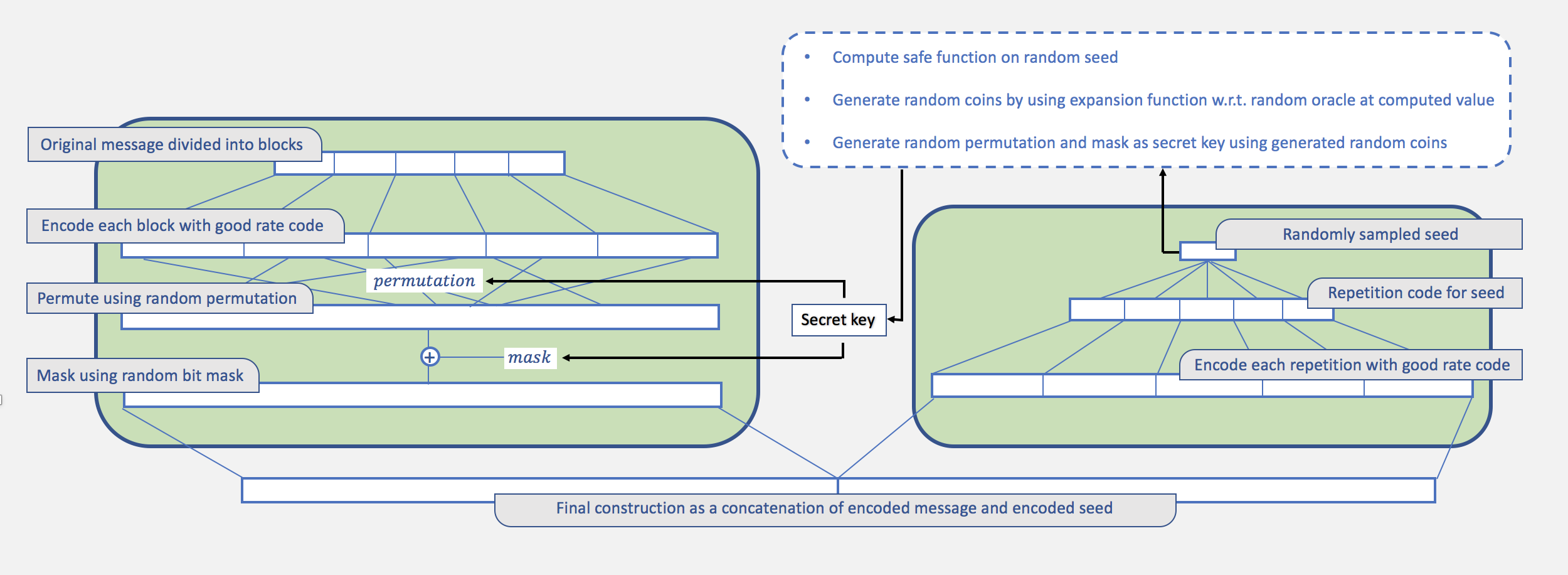
The encoding algorithm first samples a random seed of modest length (). By embedding an encoding of (via ) in our final codeword, we can ensure that our decoder will also have access to . Let the channel, over which the communication happens, belong to a class of pROM algorithms (w.r.t. random oracle ) permitting some -safe function . Even though the channel has access to the seed , it will be unable to compute by definition of the safe function. Thus is effectively a random string to the channel. We can expand this randomness via an expansion function (Definition 7), and use with this randomness to compute a key. The computed key is effectively secret from the channel and can be used in conjunction with to obtain an encoding of any input message. Note that since the decoder also has access to , it may also compute the secret key using exactly the same procedure and use this key in conjunction with to perform the required decoding. Thus the use of , safe and expansion functions on a random seed reduces the setting to that of . Our framework is parameterized by .
Explicit Constructions:
We provide explicit constructions of s against adversarial pROM channels permitting safe functions by instantiating the framework discussed above. Figure 3 gives an overview of the instantiation. For private s, we will make use of the constructions of Theorem 5. Furthermore, we instantiate as follows: The encoder encodes the seed with a standard constant rate error correcting code – we instantiate this with Justesen codes – composed with a repetition code. The local decoder then randomly samples seed-encodings and takes a majority vote over the decoded samples to determine the seed. We refer the reader to Appendix A for a formal explanation of this instantiation.
Detailed descriptions of our encoder () and decoder (), given a message , security parameter , and random oracle , may be described in Figure 4. In particular, our framework lead to the following theorem.
| o | X | X | | |
|---|---|
| 1. Sample a random seed of length . 2. Encode random seed using an . 3. Generate randomness uncomputable by channel via safe and expansion functions. 4. Generate a secret key from the randomness. 5. Use private encoder with generated key. 6. Output | 1. Decode the original random seed. 2. Compute randomness used by encoder. 3. Compute secret key used by encoder. 4. Use private decoder with computed key. Output |
Theorem 1.
Let be a private and be an . Then for any class of pROM algorithms admitting a safe function , the coding scheme in the random oracle model is an - with , , , , , . Here is an upper bound on the number of queries any algorithm makes to the random oracle .
The final codeword generated by is simply the concatenation of the codewords generated by and , resulting in . By construction, the only queries makes to the corrupted codeword are during the executions of and . This gives the locality . Furthermore for correct overall decoding, it is necessary that the individual codes are correctly decoded. Thus the total errors that the code can tolerate is bounded by the maximum number of errors any individual one of the codes can tolerate. This gives the claimed (worst case) error rate. We emphasize that the proofs of the bounds on the decoder’s success probability and the security of the framework is much more involved than the above discussion and is included in Section 3.3 and 3.4. In particular, we show that no adversary admitting -safe functions can distinguish between the encodings of and those of with random strings appended to them. Furthermore, even the decoder, who has no computational restrictions and gets the appropriate secret key used during the respective encoding processes may not make this distinction, thereby effectively reducing the security of to that of with negligible loss. The following two corollaries exhibit decoding probability vs locality tradeoffs when our framework is instantiated with the in Appendix A and the private-s of Appendix D.
Corollary 1.
For security parameter , a class of pROM adversaries admitting safe function where and for every such that where is any non-zero polynomial, there exists a coding scheme in the random oracle model that is an where (such that ), is a constant, is a constant dependent on , and . Here is a constant, is a negligible function of and is an upper bound on the total queries any algorithm in makes to the random oracle.
Corollary 2.
For security parameter , a class of pROM adversaries admitting safe function where and for every such that where is any non-zero polynomial, there exists a coding scheme in the random oracle model that is an where , is a constant, , and . Here is a constant, and are negligible functions of , and is an upper bound on the total queries any algorithm in makes to the random oracle.
Precomputation.
We remark that Steps - of may be precomputed. This may be advantageous in some settings to speed up encoding time as the sender may precompute multiple pairs. When a message is ready to be encoded, the sender then simply needs to generate using and append to generate the final codeword. However, we do note that this precomputation must be done after the selection of the random oracle, and that such precomputation is not possible for .
Multi-round Communication.
Existing constructions of private s [OPS07] are secure only for a single round of communication (see Appendix D for details on the round-based game between the encoder/decoder and the channel in the private setting). We may generalize our model to be in terms of rounds as well, where each round runs an instance of the experiment defined in Section 2.4. We remark that our codes work for this generalized model as well. In every round of the experiment, the encoder can sample a fresh random seed . This is not directly possible in the existing private constructions as an attacker listening to the decoder’s queries may learn information about the secret key after a single round of communication. For this Ostrovsky et al. introduce a new construction which hides the secret key behind a layer of encryption, which in turn increases the locality of their final constructions to .
3.3 Two-Phase Hybrid Distinguisher Argument
To prove the security of the framework in section 3.2, our approach is to argue the following: if any channel wins the LDC-Sec-Game against an instantiation of our constructions (, ), then this channel can win the priv-LDC-Sec-Game against its constituent private- (contradicting its security guarantee).
Standard Hybrid Argument Failure:
A natural attempt to prove this, yet one that fails, is to use the following standard hybrid argument. In the first hybrid we use our original encoding scheme to obtain a codeword . In the second hybrid, we replace the second component with an encoding of a random unrelated nonce to get . Here is an encoding of some random nonce which is sampled completely independent of the message encoding . We would like to argue that the two hybrids are indistinguishable and conclude that a resource bounded channel cannot fool the local decoder from original encoding scheme (first hybrid) — since we cannot fool the private- local decoder in the second hybrid. However, if the distinguisher is able to evaluate the safe-function then the hybrids are trivially distinguishably. On the other hand, if we assume that the distinguisher is resource bounded like the channel then indistinguishability does not suffice to argue that the local decoder i.e., fooling the decoder does not yield a resource bounded distinguisher since the decoder is not constrained in the same way as the resource bounded channel.
Two-Phase Argument Overview:
We address the previous issue by introducing a two-phase distinguisher game defined over adversary/distinguisher pairs. In the first phase of this game, a random coin toss randomly selects one of the hybrid encoders to encode a message. The selected hybrid hands its encoding to the adversary which outputs a corrupted codeword .
In the second phase, the distinguisher is given the initial message , the corrupted codeword , along with the secret key used to obtain , and tries to predict the value of , i.e., which hybrid encoder was used.
An important point to note is that is not constrained in any way. However, it is not given access to the random oracle.
We show (Lemma 2) that for any such attacker-distinguisher pair, the distinguisher succeeds at guessing which hybrid encoding was used with at most negligible probability.
The two phase hybrid argument allows us to reason about our original goal: the probability that the channel fools the honest decoder. In particular, a channel that wins the LDC-Sec-Game with non-negligible probability can be used in phase 1 in conjunction with a distinguisher that can simulate the decoding algorithm (with the correct key) in phase 2 to distinguish between the hybrids with non-negligible probability. This gives the required contradiction (Lemma 3). We formally define the two hybrid encoders in Figure 5.
| o | X | X | | |
|---|---|
| : (same as Figure 3) 1. Sample a random seed of length . 2. Encode random seed using an . 3. Generate randomness uncomputable by channel via safe and expansion functions. 4. Generate a secret key from the randomness. 5. Use private encoder with generated key. 6. Output | : 1. Sample a random seed of length . 2. Encode random seed using an . 3. Use private encoder with input key. 4. Output |
Let be an adversarial channel belonging to a class of pROM algorithms w.r.t random oracle permitting safe functions. Furthermore, let be a computationally unbounded algorithm. We will term and as attacker and distinguisher respectively. Using the hybrid encoders in Figure 5, we define the indistinguishability experiment over all attacker-distinguisher pairs . Note that in this experiment, is provided with the secret key that the selected hybrid used during encoding, and does not have access to the random oracle. With respect to this experiment, we define the advantage of the attacker-distinguisher pair as follows:
where the probability is taken over the randomness of , , and the selection of the random oracle . Our first aim will be to show that the advantage of any attacker-distinguisher pair, as defined above, is negligible at best.
Phase I 1. Encode message with both hybrids. Let and be the secret keys used by first and second hybrid respectively. . . 2. Flip an unbiased coin to randomly select a hybrid encoding. 3. Hand the selected encoding to the channel to get corrupted codeword. Phase II 1. Distinguisher, given the message, secret key, corrupted codeword, and security parameter, guesses the coin toss. 2.
Let be any attacker-distinguisher pair and hybrid encoders be instantiated with parameters . For security parameter and message , consider an execution of the indistinguishability experiment . Let
be the event that the attacker queries the random oracle at position where is the random seed chosen by the selected hybrid encoder and is any constant expressed in binary. Furthermore, let be the event where the attacker-distinguisher pair succeed in distinguishing the hybrid encodings in the experiment, i.e., the event where
The next proposition follows from the observation that conditioning on the event not occurring, the secret key used during the encoding process remains (information theoretically) private to both the adversary and the distinguisher. To the pair, appears information theoretically identical to which gets a secret key as its input, and thus any advantage on distinguishing the encoding schemes would allow the pair to distinguish between random strings.
Proposition 1.
The following lemma shows that the advantage for any attacker-distinguisher pair is negligible.
Lemma 2.
for any execution of the game . Here is an upper bound on the number of queries makes to the random oracle.
Proof.
Consider some execution of the game . Using conditional probability to partition the event space, the advantage of the attacker-distinguisher pair is:
By Proposition 1, we may view the event of conditioned on not occurring as an unbiased random choice. Thus . This allows us to bound the advantage of the attacker-distinguisher pair by a factor of the probability of event bad occurring by . Therefore by Lemma 1, the advantage of the attacker-distinguisher pair for the execution of is at most .
∎
3.4 Security and Decoding Probability of Constructions
Note that is identical to and is identical to with random strings appended to its output. Consider a private instance and an instantiation of our constructions . With respect to these instances, we define as the following:
Consider the codes and formed by our hybrid encoders. Here is defined identical to except that it ignores the strings appended to the output of during the encoding execution of . With respect to these codes, we define the following:
Note that by our definitions, and . The second observation follows from the following:
where the first inequality follows because , while the second inequality follows since i.e., the attacker gets to make more corruptions against . Lemma 3 upper bounds and it immediately follows that .
Lemma 3.
. Here is an upper bound on the number of queries the attacker makes to the random oracle.
Proof.
Recall that an attacker wins the if there exists some index which the corresponding decoder fails to decode with probability at least . Suppose for sake of contradiction that for some attacker . Consider the distinguisher in Figure 7. With respect to the indistinguishability experiment, takes as input the original message , the corrupted codeword , the key used by hybrid during encoding, and the security parameter .
Note that the computationally intensive step of is possible since we assume no computational restrictions. Thus by conditional probability, the advantage of distinguisher paired with any may be given by
where the penultimate equality is by definition of the distinguisher . Our initial assumption then implies that , contradicting Lemma 2. ∎
The following proposition is a direct consequence of Lemma 3 and the observation that .
Proposition 2.
where is an upper bound to the number of queries that the attacker makes to the random oracle.
Finally, we complete the proof by showing that that in Lemma 4. Combined with proposition 2 this completes the proof since .
Lemma 4.
Proof.
Let denote the event that incorrectly decodes for . We define to be the event that to simplify notation. It suffices to argue that for any since . Let be the event that recovers the correct seed from . We first observe that
Second we observe that since there are at most errors in the second part of the codeword . Finally, observe that by definition we have . The claim now directly follows. ∎
4 Constructing Safe Functions
In this section we provide several examples of safe functions in the parallel random oracle model (pROM) [AS15]. We first define the parallel random oracle model and introduce several cost metrics that measure the resources used by a pROM algorithm .
4.1 Parallel Random Oracle Model
Computation in the pROM proceeds in rounds. Each round ends when the algorithm outputs a batch of random oracle queries to be answered in parallel and a new round begins when the attacker receives the answer(s) to this batch of queries. In between rounds the may perform arbitrary computation. Formally, in the initial round the pROM algorithm takes input , performs some arbitrary computation, and outputs a state and list of random oracle queries. In general, we then have where are the answers to the random oracle queries asked in the previous round. The execution ends in round if the algorithm returns an output value along with an empty batch of random oracle queries . We use
to denote the sequence of states (and oracle queries) output when we run the pROM attacker on input fixing the random oracle and fixing ’s random coins .
Cost Metrics.
Figure 8 defines the resources we will consider as characterizing the cost of a particular execution trace . We can define the time (resp. space) cost as (resp. ). Similarly, the space time cost measures the product and cumulative memory complexity measures . Intuitively, cumulative memory complexity captures the amortized space time complexity of a function that we want to evaluate many times in parallel [AS15]. Finally, the cumulative query cost is .
| Resource | Notation | Definition |
|---|---|---|
| Time | ||
| Space | ||
| Space-Time | ||
| Cumulative memory | ||
| Cumulative query |
For a resource listed in Figure 8, the term complexity will refer to a upper bound on resource .
Definition 8.
(Resource Bounded Algorithms) We use to refer to the set of all pROM algorithms with the property that for all inputs , random oracles , and all random strings , we have . We use to refer to the subset of all pROM algorithms with the additional constraint that for all inputs , random oracles , and all random strings , we have and . Similarly, (resp. ) refers to the subset of all pROM algorithms with the additional constraint that for all inputs , random oracles , and all random strings , we have (resp. ). The definition of is symmetric — we add the additional constraint that for all .
The assumption that the channel is resource constrained with respect to one or more of the above resources (time, space, cmc, etc.) is natural in most real word settings. For example, if a low latency channel uses to compute the corruptions to an encoded message then we can plausibly assume that the attacker is time bounded — denotes the maximum number of sequential evaluations of before the corrupted codeword must be delivered. It would also be reasonable to assume that the total number of random oracle queries is polynomial in the relevant parameters. One can also argue that in most practical settings the channel will have other resource constraints e.g., space-bounded etc. In general one can define complexity classes for various combinations of resource constraints — see Definition 9.
Definition 9.
For constraints on resources listed in Figure 8, the constraint class is the set of all pROM such that is -bounded with constraints . Here, a pROM algorithm is said to be -bounded with constraints if for all and on all inputs , random coins , and random oracles , we have
SCRYPT.
Alwen et al. [ACP+17] proved that Percival’s [Per09] memory hard function is maximally memory hard. In particular, can be computed in sequential time , but any pROM attacker evaluating the scrypt function has cumulative memory complexity at least , where is the length of the output. Thus, could be used to obtain safe functions for the classes and — observe that for any execution trace .
4.2 Sequentially Hard Function
The hash iteration function , defined recursively as where , is a simple example of a safe function for the class of time bounded attackers — see Claim 1. The trade-off is sharp since it is trivial to compute in sequential time . This is a desirable property in our context since the encoder/decoder both need to compute for a random input .
We remark that the proof of Claim 1 is very similar to an argument of Cohen and Pietrzak [CP18]. Our bound is slightly tighter, but less general. Cohen and Pietrzak [CP18] proved that any pROM algorithm running in time can produce an arbitrary -sequence with probability at most . We can reduce the bound to since the attacker needs to compute a specific -sequence i.e., with . In general, we may have .
Claim 1.
Let and let then the function is -safe for the class .
Proof.
(sketch) Let . We remark that if are all distinct then
Thus, the probability of the event that for some is at most . We say that a particular random oracle query in round is lucky if the output is but the label had not previously been observed as the output to any earlier random oracle query. If denotes the maximum index such that has been observed as a random oracle output, then the probability that a particular query is lucky is at most
Conditioning on the event that no collisions occur, we can apply union bounds to show that, except with probability , there are no lucky queries. If there are no lucky queries, then after sequential rounds the output can be viewed as uniformly random and the probability that the attacker outputs is at most in this case. ∎
If we let denote the maximum number of sequential calls to that can be evaluated in a second33 3 Bonneau and Schechter [BS14] estimated that SHA256 can be evaluated times per second on a single core processor then we could set , where denotes the maximum latency of the channel. Note that the encoder/decoder would need require time marginally higher than the latency to compute .
4.3 Graph Labeling Functions
We first define a labeling function , given a graph , a hash function , and an input .
Definition 10.
Given a DAG and a random oracle function over an alphabet , we define the labeling of graph as . In particular, given an input the labeling of is defined recursively by
where are the parents of in , according to some predetermined lexicographical order. We define . If there is a single sink node then . We omit the subscripts when the dependency on the graph and hash function is clear.
The graph labeling function can be used to construct safe functions for several different classes of resource bounded adversaries. In particular, the resources necessary to compute in the pROM are tightly linked to the black pebbling cost of the DAG .
Parallel Black Pebbling Game.
A legal (parallel) pebbling of a DAG consists of a sequence of pebbling configurations — representing the set of labels which are stored in memory at time . We start with no pebbles on the graph , and can remove pebbles from the graph (free memory) at any time. For any newly pebbled node , it must be the case that where . Intuitively, this is because we cannot compute unless each of the dependent values for each is already available in memory. In the parallel version of the black pebbling game, there is no constraint on the number of new pebbles that can be placed on the graph in each round.
The space cost of a pebbling is defined as and the space complexity of a graph is . The space-time (resp. cumulative cost) cost of a pebbling is the product (resp. ). We remark that .
For constant degree graphs with nodes it is known that and that [AB16]. One can also construct graphs s.t. [ABP17, ABH17] and Paul et al. [PTC76] constructed a constant indegree graph with [PTC76, ABP18] — this last bound is tight as Hopcroft et al. [HPV77] showed that any static DAG on nodes with constant indegree can be pebbled with at most pebbles.
Pebbling Reductions.
In the appendix we prove that if and then is safe for the class . The pebbling reduction is conceptually very similar to the reduction of Alwen and Serbinenko [AS15] who proved that i.e., if the graph has high cumulative pebbling cost then is safe for the class , and by extension safe for the class . In particular, given an execution trace for an algorithm computing we can (with high probability) extract a legal pebbling for and then use an extractor argument to show that during each round — otherwise we could derive a contradiction by using the extractor to compress the random oracle. Thus, to construct a safe function one simply needs to find a graph with sufficiently large pebbling cost.
4.4 Brief Note on Candidate Constructions without Random Oracles
Recall that the proof of correctness for our constructions on space bounded channels uses the random oracle model inherently through an extractor argument showing that any space bounded channel that fools a decoding algorithm can also essentially predict a random string. However, we do not inherently require the random oracle model for general resource bounded channels. Thus in this section, we sketch candidate constructions for s on resource bounded channels that do not require the random oracle model.
In the case where the channel must forward the (corrupted) codeword to the receiver within a certain amount of time, we can use other cryptographic primitives rather than a sequence of nested hash functions. For example, time-lock puzzles [RSW96] are designed so that a sender can quickly generate a puzzle with a solution that remains hidden until some predetermined amount of time has elapsed, even if an adversary has a polynomially large number of parallel processors. On the other hand, the solution is straightforward to calculate for any honest user who has spent the desired amount of time computing the puzzle. [BGJ+16] propose time-lock puzzles through the use of succinct randomized encodings from indistinguishability obfuscation and the minimal assumption that “inherently sequential” languages exist.
For our purposes, an encoding algorithm can generate a time-lock puzzle whose solution is the random key and then transmit the time-lock puzzle along with the encoded message, using some repetition code to ensure that the time-lock puzzle can be determined by the decoding algorithm. The decoding algorithm can then solve the time-lock puzzle to obtain the random key and decode the message. However, if the channel is bounded by time and the hardness parameter of the time-lock puzzle is greater than , then the channel cannot recover the random key. It is plausible that the same construction would also yield space-bound (or space-time bound) puzzles from minimal assumptions.
Acknowledgements
We would like to thank anonymous reviewers for helpful feedback that improved the presentation of this paper. This research was supported in part by the National Science Foundation (CCF Award #1910659).
References
- [AB16] Joël Alwen and Jeremiah Blocki. Efficiently computing data-independent memory-hard functions. In Matthew Robshaw and Jonathan Katz, editors, Advances in Cryptology – CRYPTO 2016, Part II, volume 9815 of Lecture Notes in Computer Science, pages 241–271, Santa Barbara, CA, USA, August 14–18, 2016. Springer, Heidelberg, Germany.
- [ABH17] Joël Alwen, Jeremiah Blocki, and Ben Harsha. Practical graphs for optimal side-channel resistant memory-hard functions. In Bhavani M. Thuraisingham, David Evans, Tal Malkin, and Dongyan Xu, editors, ACM CCS 2017: 24th Conference on Computer and Communications Security, pages 1001–1017, Dallas, TX, USA, October 31 – November 2, 2017. ACM Press.
- [ABP17] Joël Alwen, Jeremiah Blocki, and Krzysztof Pietrzak. Depth-robust graphs and their cumulative memory complexity. In Jean-Sébastien Coron and Jesper Buus Nielsen, editors, Advances in Cryptology – EUROCRYPT 2017, Part III, volume 10212 of Lecture Notes in Computer Science, pages 3–32, Paris, France, April 30 – May 4, 2017. Springer, Heidelberg, Germany.
- [ABP18] Joël Alwen, Jeremiah Blocki, and Krzysztof Pietrzak. Sustained space complexity. In Jesper Buus Nielsen and Vincent Rijmen, editors, Advances in Cryptology – EUROCRYPT 2018, Part II, volume 10821 of Lecture Notes in Computer Science, pages 99–130, Tel Aviv, Israel, April 29 – May 3, 2018. Springer, Heidelberg, Germany.
- [ACP+17] Joël Alwen, Binyi Chen, Krzysztof Pietrzak, Leonid Reyzin, and Stefano Tessaro. Scrypt is maximally memory-hard. In Jean-Sébastien Coron and Jesper Buus Nielsen, editors, Advances in Cryptology – EUROCRYPT 2017, Part III, volume 10212 of Lecture Notes in Computer Science, pages 33–62, Paris, France, April 30 – May 4, 2017. Springer, Heidelberg, Germany.
- [AS15] Joël Alwen and Vladimir Serbinenko. High parallel complexity graphs and memory-hard functions. In Rocco A. Servedio and Ronitt Rubinfeld, editors, 47th Annual ACM Symposium on Theory of Computing, pages 595–603, Portland, OR, USA, June 14–17, 2015. ACM Press.
- [BFALS91] László Babai, Lance Fortnow, Leonid A. Levin, and Mario Szegedy. Checking computations in polylogarithmic time. pages 21–31, 01 1991.
- [BFNW91] L. Babai, L. Fortnow, N. Nisan, and A. Wigderson. Bpp has subexponential time simulations unless exptime has publishable proofs. In [1991] Proceedings of the Sixth Annual Structure in Complexity Theory Conference, pages 213–219, June 1991.
- [BGGZ19] Jeremiah Blocki, Venkata Gandikota, Elena Grigorescu, and Samson Zhou. Relaxed locally correctable codes in computationally bounded channels. In IEEE International Symposium on Information Theory, ISIT, page (to appear), 2019.
- [BGH+06] Eli Ben-Sasson, Oded Goldreich, Prahladh Harsha, Madhu Sudan, and Salil P. Vadhan. Robust pcps of proximity, shorter pcps, and applications to coding. SIAM J. Comput., 36(4):889–974, 2006. A preliminary version appeared in the Proceedings of the 36th Annual ACM Symposium on Theory of Computing (STOC).
- [BGJ+16] Nir Bitansky, Shafi Goldwasser, Abhishek Jain, Omer Paneth, Vinod Vaikuntanathan, and Brent Waters. Time-lock puzzles from randomized encodings. In Madhu Sudan, editor, ITCS 2016: 7th Conference on Innovations in Theoretical Computer Science, pages 345–356, Cambridge, MA, USA, January 14–16, 2016. Association for Computing Machinery.
- [BI01] Amos Beimel and Yuval Ishai. Information-theoretic private information retrieval: A unified construction. In Fernando Orejas, Paul G. Spirakis, and Jan van Leeuwen, editors, Automata, Languages and Programming, pages 912–926, Berlin, Heidelberg, 2001. Springer Berlin Heidelberg.
- [BS14] Joseph Bonneau and Stuart E. Schechter. Towards reliable storage of 56-bit secrets in human memory. In Kevin Fu and Jaeyeon Jung, editors, USENIX Security 2014: 23rd USENIX Security Symposium, pages 607–623, San Diego, CA, USA, August 20–22, 2014. USENIX Association.
- [CKGS98] Benny Chor, Eyal Kushilevitz, Oded Goldreich, and Madhu Sudan. Private information retrieval. J. ACM, 45(6):965–981, November 1998.
- [CMS99] Christian Cachin, Silvio Micali, and Markus Stadler. Computationally private information retrieval with polylogarithmic communication. In Advances in Cryptology - EUROCRYPT ’99, International Conference on the Theory and Application of Cryptographic Techniques, Prague, Czech Republic, May 2-6, 1999, Proceeding, pages 402–414, 1999.
- [CP18] Bram Cohen and Krzysztof Pietrzak. Simple proofs of sequential work. In Jesper Buus Nielsen and Vincent Rijmen, editors, Advances in Cryptology – EUROCRYPT 2018, Part II, volume 10821 of Lecture Notes in Computer Science, pages 451–467, Tel Aviv, Israel, April 29 – May 3, 2018. Springer, Heidelberg, Germany.
- [DGY11] Zeev Dvir, Parikshit Gopalan, and Sergey Yekhanin. Matching vector codes. SIAM J. Comput., 40(4):1154–1178, 2011.
- [DJK+02] A. Deshpande, R. Jain, T. Kavitha, S. V. Lokam, and J. Radhakrishnan. Better lower bounds for locally decodable codes. In Proceedings 17th IEEE Annual Conference on Computational Complexity, pages 184–193, May 2002.
- [DKW11] Stefan Dziembowski, Tomasz Kazana, and Daniel Wichs. One-time computable self-erasing functions. In Theory of Cryptography - 8th Theory of Cryptography Conference, TCC Proceedings, pages 125–143, 2011.
- [Efr12] Klim Efremenko. 3-query locally decodable codes of subexponential length. SIAM J. Comput., 41(6):1694–1703, 2012.
- [GLR+91] Peter Gemmell, Richard Lipton, Ronitt Rubinfeld, Madhu Sudan, and Avi Wigderson. Self-testing/correcting for polynomials and for approximate functions. In Proceedings of the Twenty-third Annual ACM Symposium on Theory of Computing, STOC ’91, pages 33–42, New York, NY, USA, 1991. ACM.
- [GRR18] Tom Gur, Govind Ramnarayan, and Ron D. Rothblum. Relaxed locally correctable codes. In 9th Innovations in Theoretical Computer Science Conference, ITCS, pages 27:1–27:11, 2018.
- [GS16] Venkatesan Guruswami and Adam Smith. Optimal rate code constructions for computationally simple channels. J. ACM, 63(4):35:1–35:37, September 2016.
- [HO08] Brett Hemenway and Rafail Ostrovsky. Public-key locally-decodable codes. In Advances in Cryptology - CRYPTO 2008, 28th Annual International Cryptology Conference, Proceedings, pages 126–143, 2008.
- [HOSW11] Brett Hemenway, Rafail Ostrovsky, Martin J. Strauss, and Mary Wootters. Public key locally decodable codes with short keys. In 14th International Workshop, APPROX, and 15th International Workshop, RANDOM, Proceedings, pages 605–615, 2011.
- [HPV77] John Hopcroft, Wolfgang Paul, and Leslie Valiant. On time versus space. J. ACM, 24(2):332–337, April 1977.
- [Jus72] J. Justesen. Class of constructive asymptotically good algebraic codes. IEEE Transactions on Information Theory, 18(5):652–656, Sep. 1972.
- [KdW04] Iordanis Kerenidis and Ronald de Wolf. Exponential lower bound for 2-query locally decodable codes via a quantum argument. J. Comput. Syst. Sci., 69(3):395–420, 2004.
- [KMRS17] Swastik Kopparty, Or Meir, Noga Ron-Zewi, and Shubhangi Saraf. High-rate locally correctable and locally testable codes with sub-polynomial query complexity. J. ACM, 64(2):11:1–11:42, 2017.
- [KO97] E. Kushilevitz and R. Ostrovsky. Replication is not needed: single database, computationally-private information retrieval. In Proceedings 38th Annual Symposium on Foundations of Computer Science, pages 364–373, Oct 1997.
- [KT00] Jonathan Katz and Luca Trevisan. On the efficiency of local decoding procedures for error-correcting codes. In Proceedings of the Thirty-second Annual ACM Symposium on Theory of Computing, STOC ’00, pages 80–86, New York, NY, USA, 2000. ACM.
- [Lip94] Richard J. Lipton. A new approach to information theory. In STACS 94, pages 699–708, Berlin, Heidelberg, 1994.
- [MPSW05] Silvio Micali, Chris Peikert, Madhu Sudan, and David A. Wilson. Optimal error correction against computationally bounded noise. In Joe Kilian, editor, Theory of Cryptography, pages 1–16, Berlin, Heidelberg, 2005. Springer Berlin Heidelberg.
- [OPS07] Rafail Ostrovsky, Omkant Pandey, and Amit Sahai. Private locally decodable codes. In Automata, Languages and Programming, pages 387–398, 2007.
- [Per09] C. Percival. Stronger key derivation via sequential memory-hard functions. In BSDCan 2009, 2009.
- [PTC76] Wolfgang J. Paul, Robert Endre Tarjan, and James R. Celoni. Space bounds for a game on graphs. In Proceedings of the Eighth Annual ACM Symposium on Theory of Computing, STOC ’76, pages 149–160, New York, NY, USA, 1976. ACM.
- [RSW96] Ronald L Rivest, Adi Shamir, and David A Wagner. Time-lock puzzles and timed-release crypto. 1996.
- [SS16] Ronen Shaltiel and Jad Silbak. Explicit list-decodable codes with optimal rate for computationally bounded channels. In Approximation, Randomization, and Combinatorial Optimization. Algorithms and Techniques, APPROX/RANDOM, pages 45:1–45:38, 2016.
- [STV01] Madhu Sudan, Luca Trevisan, and Salil Vadhan. Pseudorandom generators without the xor lemma. Journal of Computer and System Sciences, 62(2):236 – 266, 2001.
- [Yek08] Sergey Yekhanin. Towards 3-query locally decodable codes of subexponential length. J. ACM, 55(1):1:1–1:16, 2008.
Appendix A Repetition with Justesen Codes
As a preliminary to this section, we require familiarity with the following form of standard one-sided Chernoff Bounds.
Proposition 3 (Chernoff Bound).
Let be independent random variables such that for each . Let and . Then for any ,
In this section, we will describe our encoding scheme in order to recover the random seed used by our main constructions in Section 3.2. Recall that our approach was to encode using a repetition code by repeating multiple () times, and then encoding each repetition of into using an off-the-shelf error correcting code with constant error and information rates. While any constant rate error correcting code may be used, we make use of Justesen Codes:
Theorem 2.
[Jus72] For any , there exist binary linear codes of rate , that are efficiently decodable from fraction of errors, where is a function that only depends on .
We will denote as the code that achieving the guarantees of Theorem 2, i.e. having constant rate and error correction rate . Let denote the length of these codewords. We now give our code constructions to recover via repetition with Justesen codes.
(): 1. . 2. where is repeated times for a fixed . 3. OutputThe following lemma states that the code may be used to recover the original with high probability using good locality.
Lemma 5.
Let be as in Theorem 2 and be the number of samples that makes to the corrupted codeword. Then for all , the coding scheme is an - where , is some constant, and .
Proof.
The adversary makes a total of corruptions to . Let . By Theorem 2, for a block to be non-decodable by , the adversary must make at least corruptions in this block. This allows us to bound the total blocks the adversary may corrupt as at most . Thus the probability of sampling a block that is non-decodable is at most . Setting , we get that the probability of sampling a block that may be recovered is at least . Let denote the number of samples that are successfully recovered. Thus, and by standard Chernoff Bounds (Proposition 3), we have that
Note that if , then our majority vote succeeds in determining the original message. Thus . Finally, each block has size . Since we sample blocks, we get the claimed locality. ∎
Appendix B Memory Bounded Adversary
In this section we show that the memory complexity of the function is characterized by the space cost in the parallel random oracle model just as Alwen and Serbinenko [AS15] showed that cumulative memory complexity can be characterized by the black pebbling game.
Graph Pebbling
Given a directed acyclic graph (DAG) , the goal of the (parallel) black pebbling game is to place pebbles on all sink nodes of (not necessarily simultaneously). The game is played in rounds and we use to denote the set of currently pebbled nodes on round . Initially all nodes are unpebbled, , and in each round we may only include if all of ’s parents were pebbled in the previous configuration () or if was already pebbled in the last round ().
The cumulative cost of the pebbling is defined to be . Graph pebbling is a particularly useful as a tool to analyze the security of an iMHF [AS15]. A pebbling of naturally corresponds to an algorithm to compute the iMHF. Alwen and Serbinenko [AS15] proved that in the parallel random oracle model (pROM) of computation, any algorithm evaluating such an iMHF could be reduced to a pebbling strategy with (approximately) the same cumulative memory cost.
However for our purposes, we are more concerned about the space cost rather than the cumulative memory cost. The space of the pebbling is defined to be and accordingly, , where the minimum is taken over all valid pebblings .
Reduction
Similar to [AS15] our reduction uses Lemma 6 as a core building block. In particular, if the space complexity is significantly smaller than for a pROM attacker then we will be able to build an extractor that receives a small hint and predicts the random oracle output on an index contradicting Lemma 6. By contrast, a black pebbling move always corresponds to a specific random oracle query.
Lemma 6.
[DKW11] Let be a series of random bits and let be an algorithm that receives a hint and can query at specific indices. If outputs a subset of indices of that were previously not queried, as well as guesses for each of the bits, the probability there exists some so that all the guesses are correct is at most .
B.1 Memory and Cache in the Parallel Random Oracle Model
Before we present our reduction, we first recall the formal definition of space complexity in the pROM model. Let the state of an algorithm at time to be , which contains the contents of the memory. Let be a pROM attacker who is given oracle access to a random oracle . An execution of on input proceeds in rounds as follows. Initially, the state at time is , which encodes the initial input . At the beginning of round the attacker is given the initial state as well as the answers to any random oracle queries that were asked at the end of the last round. The algorithm may then perform arbitrary computation and choose to update the memory, outputting a new state , along with a batch of queries .
Execution Trace.
Recall that the execution trace of the algorithm is defined by the sequence of memory states and queries made to the random oracle . Formally, the execution trace is , where the trace is dependent on the algorithm , random oracle , internal randomness , and input value . Then the memory cost of the execution trace is
Recall that Alwen and Serbinenko [AS15] show that the computation of a function with hash function and underlying directed acyclic graph yields a legal black pebbling with high probability. Thus, we use to extract a legal . Given an execution trace , the corresponding pebbling is defined by setting and define the pebbles at each subsequent time step based on the corresponding batch of queries made during iteration . We then apply the following rules:
- •
For each query in batch , if the query has the form for some vertex and its parents , then we add a pebble to node in .
- •
If there exists another query for before is used as input for a query, then is deleted from .
Intuitively, at each time , contains all nodes whose label will appear as input to a future random oracle query before the label appears as the output of a random oracle query. In this manner, we define , which Alwen and Serbineneko show is legal with high probability:
Theorem 3.
[AS15] The pebbling extracted from an execution trace,
is a legal black pebbling with probability at least , where is the label size and is the number of queries made by .
We now show that any algorithm that computes correctly with probability at least has memory cost dependent on the space complexity of the resulting legal black pebbling, . The proof uses that fact that if an attacking strategy does not yield a corresponding legal black pebbling, then the attacking strategy can be modified to form an extractor for the labels of a subset of nodes. Specifically, an extractor with access to the attacking strategy, the state of the memory, and a few select hints can successfully predict a large number of random bits, which cannot happen with high probability. The hints given to the extractor describes the positions of the random bits, and ensure these bits remain “random” (that is, we do not explicitly query these locations later). In particular, the extractor uses the hints to simulate but the hints do not include the current state of memory .
Theorem 4.
Let be a DAG with nodes, , , and be a fixed input. Let . For any algorithm that makes at most queries, let be the event that the attacker either uses in its computation of or fails to compute the function correctly. Then
Proof.
Consider an instance of that succeeds in calculating , making at most queries. By Theorem 3, with probability at least , we can extract a legal black pebbling from . Conditioned on the success of the extraction of a legal black pebbling, let be the space complexity of the execution trace of the evaluation algorithm. By definition of , there exists a time step such that the corresponding legal black pebbling contains at least pebbles. Suppose, by way of contradiction, that so that . By construction of the pebbling, there is a set containing labels that appear as input for a query after time step before they are returned as output. Moreover, there are collisions among labels with probability at most , so conditioned on the event that there are no collisions among the labels, then the algorithm would have to generate the labels out of thin air. Specifically, an extractor using will be able to predict labels, each of size bits, using a bits of information from the state of , along with the following hint, which consists of three parts:
- 1.
The set is given as a hint to denote the indices that form the string that the extractor will ultimately predict. Since contains positions, then the size of this component of the hint is bits.
- 2.
For each , the index of the first query that appears in which is needed as input. This component of the hint tells the extractor the queries that require the prediction of random strings, and has size at most bits, where is the total number of queries made by the attacker.
- 3.
For each , the index of the first query when might be compromised. Observe that if the extractor successfully predicts a random string at a location , but then is later queried by the attacker, we cannot distinguish this case at the end from the case that the extractor simply read after making the query. Effectively, the extractor is no longer predicting a random string. To avoid this, the hint given to the extractor details queries that would compromise the randomness of the desired locations. Formally, the hint is the minimal index such that , which yields returns the query . This component of the hint tells the extractor the locations of the random strings to be predicted, and has size at most bits.
See Figure 9 for intuition.
The size of the hint is at most bits. However, the extractor is able to use to predict fresh input/output pairs from the random oracle. That is, the extractor can predict labels of length from the random oracle for a total of random bits from bits. Thus for and , the extractor predicts random bits from random bits, which can only occur with probability by Lemma 6. Hence, the probability that the attacker either uses in its computation of or fails to compute the function correctly is at least , where the possible events of failure are the inability to extract a legal pebbling from the attacker, the probability of extracting random bits from random bits, and collisions among the labels, respectively. ∎
Appendix C Code Scrambling
Code scrambling was a technique introduced by Lipton [Lip94] for transforming codes designed for the symmetric channel, to be used against any PPT adversarial channel. Assume that the sender and receiver share some private randomness . Here is a random permutation on and is a random mask. is then length of the encoding obtained by , a constant rate code in the symmetric channel. Consider the following code against the PPT adversarial channel: given message ,
The key observation is that and are independent due to . This may be observed by considering a specific and realizing that the final encoding may take on any values due to the . Thus if the error vector added by the adversarial channel is , then we have
Thus the errors added are random, due to the random permutation, and may recover the original message.
Appendix D Private s
Private locally decodable codes were introduced by Ostrovsky, Pandey and Sahai [OPS07]. These s are termed private as they crucially assume a secret key given to both the sender and the receiver before the protocol, but kept private from the PPT channel.
Definition 11.
Let be the security parameter. A private -locally decodable code for a parameters , is a triplet of probabilistic polynomial time algorithms such that:
- •
is the key generation algorithm that takes as input the security parameter and outputs a secret key .
- •
is the encoding algorithm that takes as input the message of length and the secret key . The algorithm outputs that denotes an encoding of .
- •
denotes the decoding algorithm, which takes as input a bit position and the secret key . It outputs a single bit denoting the decoding of by making at most (adaptive) queries into a given a codeword possibly different from .
Here, denotes the query complexity or locality of the code and is termed the error rate.
Furthermore, we say that the private decodes with probability if for PPT channels in the experiment of definition 12 (defined below) for all and , we have
The game between the encoder/decoder and PPT adversarial channel may be described as follows:
Definition 12.
A computationally bounded adversarial channel with error rate is a probabilistic polynomial time algorithm which repeatedly interacts with the encoding algorithm and the decoding algorithm polynomially many times until it terminates. Each iteration takes place as follows:
- 1.
Given a security parameter , the key generation algorithm outputs a secret key . The secret is given to both the sender (encoder) and the receiver (decoder) but not to the channel. The channel is given .
- 2.
In the iteration, the channel chooses a message and hands it to the sender.
- 3.
The sender computes and hands the codeword back to the channel.
- 4.
The channel corrupts at most a fraction of all bits in to output the corrupted codeword , i.e., . It gives and a challenge bit to the receiver’s
- 5.
The receiver makes at most (possibly adaptive) queries into the new codeword and outputs .
Using such a setup, Ostrovsky et al. give explict constructions of one-time private s i.e. s that may be used for exactly one-round of communication in definition 12. They achieve this by code scrambling (Appendix C) a simple repetition code of the original message. Good locality is then achieved by reading and unscrambling only the bits exactly corresponding to indices of repetitions of the queried bit. It turns out that this simple code does not have good rate as the number of repetitions that need to be applied per symbol of the original message in the repetition code is not constant. Due to this, the authors employ a strategy where the message to be encoded is divided into blocks of small size. Each block is then encoded using an error correcting code of constant rate, and then the concatenation of all the encoded blocks is scrambled using the secret key. Good locality is achieved by reading and unscrambling only the bits exactly corresponding to the block containing the queried bit. Specifically, Ostrovsky et al. give constructions of private over the binary alphabet and show the following against adversarial channels:
Theorem 5 ([OPS07]).
Let be any function such that . Then, there exists a constant such that is a one time private -locally decodable code with and constant information rate that correctly decodes from error rate with probability at least .
In Section 2.3, we introduce Definition 4 as an alternative to working with Definitions 11 and 12. Furthermore, we make use of this alternative definition of private-s throughout the main sections. We thus present Theorem 5 in an alternative form where private s are presented as Definition 4. We use this in instantiating our framework in Section 3.2 (Corollaries 1 and 2).
Theorem 6 (Alternative to Theorem 5).
Let be any function such that . Then, for security parameter and for all such that where is any non-zero polynomial, there exists a coding scheme that is a one-time private where , is a constant, , and is negligible in the security parameter.