Topological Spaser

The concept of the surface plasmon amplification by stimulated emission of radiation (spaser, also called plasmonic nanolaser) Bergman and Stockman 2003; Stockman and Bergman 2009; Stockman 2010 has recently been experiencing rapid development. Many different types of spasers have been proposed Li et al. 2005; Fedyanin 2012; Baranov et al. 2013; Zheludev et al. 2008 and demonstrated Noginov et al. 2009; Oulton et al. 2009; Ma et al. 2010; Flynn et al. 2011; Marell et al. 2011; v. Beijnum et al. 2013; Lu et al. 2014; Zhang et al. 2014; Chou et al. 2016; Lee et al. 2017; Sun et al. 2017. The spasers were also applied to various problems including explosives detection Ma et al. 2014, monitoring of the nano-environment Wang et al. 2017a; Wang et al. 2017b, cancer therapeutics and diagnostics (theranostics) Galanzha et al. 2017.

A particular type of the spasers is represented by plasmonic crystals that include gain media Zheludev et al. 2008; Zhou et al. 2013; Stockman 2013; v. Beijnum et al. 2013. Such spasers belong to the class of lasing spasers Zheludev et al. 2008, which are nanostructured plasmonic metasurfaces consisting of a periodic lattice of individual spasers. Due to interactions in the near-field, the individual spasers lock in phase to generate temporaly- and spatially-coherent fields. However, such a fundamental question as the effects of topological properties (the Berry curvature) Berry 1984; Xiao et al. 2010 of the plasmonic Bloch bands of such crystals has not yet been investigated.

Recently, a groundbreaking work has been carried out aimed at obtaining a topological lasing in a plasmonic-photonic (diffractive) lattice of honeycomb symmetry Guo et al. 2019. The plasmonic lasing was observed at the $\mathbf{K}$-points but only in a mode of the $A_{1}^{\prime}$ symmetry, which is a singlet (scalar) representation. Therefore, this mode does not possess a chiral topological charge.

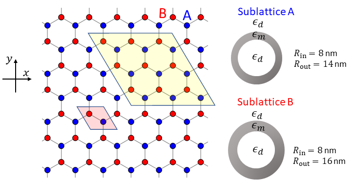
In this Letter, we propose a topological spaser that geometrically is a deeply-subwavelength two-dimensional (2d) crystal (metasurface) with a honeycomb symmetry built of two different triangular sublattices, $\mathrm{A}$ and $\mathrm{B}$ – see Fig. 1. A metaatom of such a lattice is a plasmonic metal nanoshell containing an achiral gain medium, similar to the spaser geometry of Ref. Stockman 2010. The $\mathrm{A}$- and $\mathrm{B}$-sublattices of such a topological spaser differ in size and shape of the constituent nanoshells (see the caption to Fig. 1), so their individual spasers have different eigenfrequencies. Note that a natural example of a honeycomb lattice consisting of two different sublattices is provided by the transition metal dichalcogenide (TMDC) crystals You et al. 2015; Novoselov et al. 2016; Basov et al. 2016.

The spasing eigenmodes are surface plasmons (SPs) that should be classified corresponding to irreducible representations of the symmetry point group of the lattice unit cell, which is $D_{3h}$ Landau and Lifshitz 1965. This group has six representations, of which $E^{\prime}$ is a two-dimensional (doublet) representation with the desired properties – see Appendix. It describes two degenerate modes time-reversed to each other, which carry topological charges of $Q_{T}=\pm 1$ defining their chirality; their local fields rotate in time and space in the opposite directions.

For the proposed topological spaser, we will show that the degenerate eigenmodes at the $\mathbf{K}$- and $\mathbf{K}^{\prime}$-points strongly compete with each other, making such a topological spaser bistable: either $Q_{T}=1$ or $Q_{T}=-1$ mode can generate. These spasing modes are topological Berry plasmons Song and Rudner 2016. However, in Ref. Song and Rudner 2016, the system’s chirality was due to the induced valley polarization. In a sharp contrast, in our case the system is originally achiral and $\mathcal{T}$-reversible: no integral Berry curvature or magnetic field are present; the chirality is self-organized due to the mode competition causing a spontaneous violation of the $\mathcal{T}$-reversal and $\sigma_{v}^{\prime}$-reflection symmetries.

The quasistatic SPs eigenmodes Bergman and Stroud 1992 are electric potentials, $\varphi_{\nu\mathbf{k}}(\mathbf{r})$, characterized by lattice momentum $\mathbf{k}$ and band index $\nu$. These eigenmodes can be found from the quasistatic equation Stockman et al. 2001

where $1>s_{\nu\mathbf{k}}>0$ are the eigenvalues, and $\Theta(\mathbf{r})$ is the characteristic function, which is 1 inside and 0 outside the metal. These eigenmodes satisfy an orthonormality condition: $\int\nabla\varphi_{\nu\mathbf{k}}\nabla\varphi_{\nu^{\prime}\mathbf{k}^{\prime}}^{\ast}d^{3}r=\delta_{\nu\nu^{\prime}}\delta_{\mathbf{k}\mathbf{k}^{\prime}}$.

We employ the tight-binding approximation where the on-site states are the modes of isolated metal nanoshells, and the coupling between them is the nearest-neighbor dipole interaction. For each nanoshell, we consider two eigenmodes constituting a basis for the $E^{\prime}$ doublet representation of the $D_{3h}$ point symmetry group, $\varphi^{(\alpha)}_{m}\propto Y_{1m}$, where $Y_{1m}$ are the spherical harmonics, $m=\pm 1$, and $\alpha=\mathrm{A}$ or $\mathrm{B}$. These eigenmodes with $m=\pm 1$ have the electric field components in the $xy$-plane of the lattice and are coupled by the dipole interaction.

The eigenmodes $\varphi^{(\alpha)}_{m}$ of an isolated nanoshell of a sublattice $\alpha=\mathrm{A},\mathrm{B}$ satisfy the following equation [cf. Eq. (1)]

where $\Theta^{(\alpha)}(\mathbf{r})$ is 1 inside the metal of nanoshell $\alpha$ and 0 elsewhere, and $\mathbf{r}$ is relative to the center of this nanoshell. The solution of Eq. (2) can be expressed as an expansion over the spherical harmonics, $Y_{1m}$, see Appendix.

With the known eigenmodes of the isolated nanoshells, we express the quasistatic potential for a mode with quantum numbers $\nu,\mathbf{k}$ as a sum over the lattice and $m=\pm 1$,

where $\mathbf{R}^{(\alpha)}_{j}$ is the lattice vector of the nanoshell $j$ center in sublattice $\alpha$. Expansion coefficients $C^{(\alpha)}_{\nu\mathbf{k}m}$ satisfy the following tight-binding equations

Here the nearest neighbor tight-binding Hamiltonian is

where $j$ is an arbitrary lattice site, and $j^{\prime}$ are the nearest-neighbor sites to it.

The solution of Eq. (4) produces four bands whose dispersions are shown in Fig. 2(a). Due to the broken inversion symmetry owing to the sublattices A and B being inequivalent, there are band gaps opened at the $\mathbf{K}$- and $\mathbf{K}^{\prime}$-points.

The structure of SP excitations at these points is the following. At either the $\mathbf{K}$-point or the $\mathbf{K}^{\prime}$-point, the SP modes are excited in the real space only on a single sublattice, $A$ – see an illustration in Fig. 2(b). The SPs at the $\mathbf{K}$- and $\mathbf{K}^{\prime}$-points are mutually time-reversed: the magnetic quantum numbers are $m=\pm 1$ corresponding to the topological charges $Q_{T}=\pm 1$, and the phase shifts between the nearest sites on the $A$ sublattice are $\pm 2\pi/3$, respectively, as illustrated in Fig. 3(a)-(d). Below we assume that the frequency of the optical transitions in the gain medium is equal to the frequency of SPs in the valence band at the $\mathbf{K}$- and $\mathbf{K}^{\prime}$-points – see a schematic in Fig. 3(e).

The SP’s at the $\mathbf{K}$- and $\mathbf{K}^{\prime}$-points have equal frequencies, $\omega_{\nu\mathbf{K}}=\omega_{\nu\mathbf{K}^{\prime}}$, as protected by the $\mathcal{T}$ symmetry. We write down the Hamiltonian of the plasmonic system in the second quantization as

where $\hat{a}_{\nu\mathbf{k}}^{\dagger}$ and $\hat{a}_{\nu\mathbf{k}}$ are the SP creation and annihilation operators. Here the frequency $\omega_{\nu\mathbf{k}}$ is found from equation Re$[s(\omega_{\nu\mathbf{k}})]=s_{\nu\mathbf{k}}$, where $s(\omega)=\epsilon_{d}/(\epsilon_{d}-\epsilon_{m}(\omega))$ is the Bergman spectral parameter, $\epsilon_{d}$ and $\epsilon_{m}(\omega)$ are the dielectric functions of the host material and the metal, respectively. The corresponding electric field is given by Bergman and Stockman 2003

where $A_{\nu\mathbf{k}}=\sqrt{\left.4\pi\hbar s_{\nu\mathbf{k}}\right/{\epsilon_{d}s_{\nu\mathbf{k}}^{\prime}}}$, $s_{\nu\mathbf{k}}^{\prime}=\mathrm{Re}[{ds(\omega)}/{d\omega}|_{\omega=\omega_{\nu\mathbf{k}}}]$.

The gain medium is assumed to be achiral with a linear transition dipole moment $\mathbf{d}$; this dipole equally couples to both the $\mathbf{K}$ and $\mathbf{K}^{\prime}$ SP modes. The gain medium is described quantum mechanically using density matrix $\rho^{(p)}$ for a $p$th nanoshell. Within the rotating wave approximation (RWA), the non-diagonal elements of the density matrix can be written as $(\rho^{(p)})_{12}=\bar{\rho}^{(p)}\exp(i\omega_{\nu\mathbf{K}}t)$, while the diagonal elements determine the population inversion, $n^{(p)}=\rho^{(p)}_{22}-\rho^{(p)}_{11}$. The interaction between the gain medium and the SP system is determined by Hamiltonian

Following Ref. Stockman 2010, we treat the plasmonic field quasiclassically by replacing the creation and annihilation operators of the SP’s by the respective complex $c$-number amplitudes $a_{\nu\mathbf{K}}^{\ast}$, $a_{\nu\mathbf{K}}$, and $a_{\nu\mathbf{K}^{\prime}}^{\ast}$, $a_{\nu\mathbf{K}^{\prime}}$. The corresponding SP population numbers per the composite unit cell are $N_{\mathbf{K}}=\left|a_{\nu\mathbf{K}}\right|^{2}$ and $N_{\mathbf{K}^{\prime}}=\left|a_{\nu\mathbf{K}^{\prime}}\right|^{2}$.

The coupled system of equations Stockman 2010, which describes both the SPs and the gain medium, takes the following form

where $N_{g}$ is the number of electrons of the gain medium inside each shell, $\gamma_{sp}$ is the SP relaxation rate, $\gamma_{2}$ is the non-radiative decay rate of the level $|2\rangle$ of the chromophore, $\Gamma_{12}$ is polarization relaxation rate for the $|2\rangle\to|1\rangle$ transition of the chromophores, $g$ is the excitation (pumping) rate per a chromophore, and $\tilde{\Omega}_{\nu\mathbf{k}}^{(p)}=\frac{1}{\hbar}A_{\nu\mathbf{k}}\nabla\varphi_{\nu\mathbf{k}}(\mathbf{r}^{(p)})\mathbf{d}^{(p)}$ is the Rabi frequency. In computations, we set: $\epsilon_{d}=2$, $d=10$ debye, $N_{\mathrm{g}}=514$, $\gamma_{\mathrm{sp}}=4.1\times 10^{13}$ $\mathrm{s^{-1}}$, $\Gamma_{12}=2.1\times 10^{14}$ $\mathrm{s^{-1}}$, and $\gamma_{2}=4\times 10^{12}$ $\mathrm{s^{-1}}$. We used dielectric data Johnson and Christy 1972 for silver as the nanoshells’ metal.

The Rabi frequencies, $\tilde{\Omega}_{\nu\mathbf{K}}^{(p)}$ and $\tilde{\Omega}_{\nu\mathbf{K}^{\prime}}^{(p)}$, are periodic with respect to the position vector, $\mathbf{r}^{(p)}$, with the periods that are determined by the crystal momenta $\mathbf{K}$ and $\mathbf{K}^{\prime}$, respectively. Any solution of Eqs. (9)-(12), which contains both the $\mathbf{K}$ and $\mathbf{K}^{\prime}$ components, will be periodic on a superlattice with an eighteen-nanoshell unit cell (“supercell”) shown in Fig. 1. Then the summation over $p$ in Eqs. (9) and (10) is extended over the corresponding eighteen points.

As initial conditions for Eqs. (9)-(12), we set $n^{(p)}(t)|_{t=0}=-1$, which implies that initially all the chromophores of the gain medium are in the ground state. Similarly, we assume that initially there is no polarization, $\bar{\rho}(t)|_{t=0}=0$. With respect to the initial SP amplitudes, $a_{\nu\mathbf{K}}$ and $a_{\nu\mathbf{K}^{\prime}}$, we consider three cases: (i) The initial SP amplitude is small and located only at the $\mathbf{K}$-point where we set $a_{\nu\mathbf{K}}=0.1$ and $a_{\nu\mathbf{K}^{\prime}}=0$; (ii) The same as the previous case but with the SP amplitude located at the $\mathbf{K}^{\prime}$-point, $a_{\nu\mathbf{K}}=0$ and $a_{\nu\mathbf{K}^{\prime}}=0.1$; (iii) The SP’s are initially present at both the $\mathbf{K}$- and $\mathbf{K}^{\prime}$-points but with different amplitudes, $a_{\nu\mathbf{K}}=1$ and $a_{\nu\mathbf{K}^{\prime}}=0.2$.

We start with case (iii) where initially both the $\mathbf{K}$- and $\mathbf{K}^{\prime}$-valleys are weakly populated, with a higher population at the $\mathbf{K}$-point, which emulates a random initial condition created by quantum fluctuations. The pumping begins at $t=0$ with a rate of $g=10^{13}$ $\mathrm{s^{-1}}$. The dynamics of the SP populations in both the valleys as a function of time $t$ after the beginning of the pumping is displayed in Fig. 4(a). As we see, after the initial period of decay and relaxation oscillations, the population of the dominant $\mathbf{K}$-valley starts growing exponentially and then levels off becoming stationary with the SP population $N_{\mathbf{K}}\approx 150$. At the same time, the minor SP population, $N_{\mathbf{K}^{\prime}}$, decays exponentially for $t\gtrsim 200$ fs. This occurs due to a strong competition of the $\mathbf{K}$- and $\mathbf{K}^{\prime}$-modes for the common gain. At the same time, the decay to zero, $N_{\mathbf{K}^{\prime}}\to 0$, implies that there is no cross-mode talk, which is due to the topological protection: these two SP modes carry conserved topological charges $Q_{T}=\pm 1$. Due to the $\mathcal{T}$-symmetry, the valleys are symmetric: starting with the $\mathbf{K}^{\prime}$-valley with a dominant SP population, the final population will only be in that valley. Thus the topological spaser is a topologically-protected symmetric bistable device.

The kinetics of the topological spaser, i.e., the dependence of the stationary SP population numbers, $N_{\mathbf{K}}$ and $N_{\mathbf{K}^{\prime}}$ for $t\to\infty$, as functions of the pumping rate $g$, is illustrated in Fig. 4(b) for case (i) when only the $\mathbf{K}$-valley has a non-zero initial population: $N_{\mathbf{K}}=0.01$ and $N_{\mathbf{K}^{\prime}}$=0. There is a pronounced threshold after which the SP population in the $\mathbf{K}$-valley grows linearly with the pumping rate. The population in the $\mathbf{K}^{\prime}$-valley remains zero due to the topological protection. Similarly, in case (ii), the SP population will be amplified and remain only in the $\mathbf{K}^{\prime}$-valley.

The dynamics of the real-space distributions of the local fields in the topological spaser is shown in Fig. 6 (a)-(e) for the case of the $\mathbf{K}$-valley generation (see also Appendix for the $\mathbf{K}^{\prime}$ mode). The fields are normalized to one SP in the unit supercell. This distribution contains three dipolar fields localized on the A-sublattice nanoshells, which rotate clockwise in the optical cycle. This field distribution is generally chiral and compliant with the $E^{\prime}$ representation of the $D_{3h}$ group. At a given moment of time, this field distribution can also be described as a chiral lattice wave propagating in the clockwise direction along the unit cell boundary. The 2d $E^{\prime}$ representation also describes a mode with the opposite (counter-clockwise) chirality, which can be obtained by an application of either $\mathcal{T}$ or $\sigma_{v}^{\prime}$ symmetry operations.

The present topologically-charged $E^{\prime}$ spasing mode is indeed dark: obviously, it does not possess a net dipole moment. However, there is a non-zero chiral current propagating unidirectionally clockwise (for $Q_{T}=1$) or counterclockwise (for $Q_{T}=-1$) within the A-sublattice unit cell. Such currents for the neighboring cells cancel out each other. However, there will be an uncompensated chiral current at the edge of the 2d plasmonic lattice, which is illustrated in Fig. 6 (e). The corresponding local fields resemble a field of a plasmon polariton propagating clockwise along the edge despite the absence of the edge states, similar to the edge plasmon polaritons in Ref. Song and Rudner 2016.

There is the second $E^{\prime}$ mode of the same frequency, which is related to the above-discussed right-rotating one by the application of either $\mathcal{T}$ or $\sigma_{v}^{\prime}$ symmetry operations. That mode is generated in the $\mathbf{K}^{\prime}$-valley; it is rotating counter-clockwise within the unit cell and propagating counter-clockwise along the edge. The choice of which one of these modes will be generated is random and is a spontaneous violation of the $\mathcal{T}$ and $\sigma_{v}^{\prime}$ symmetries.

In conclusion, we propose a topological spaser constituted by a honeycomb lattice of spherical metal nanoshells containing a gain medium. The two sublattices, A and B, are built from two different types of nanoshells. Such a spaser generates one of two chiral plasmonic modes characterized by topological charge $Q_{T}=\pm 1$ whose local fields rotate clockwise or counter-clockwise, respectively. Which of these two modes is generated is determined by a spontaneous violation of symmetry as defined by the initial conditions. The chirality of the spasing mode is stable and topologically protected. The macroscopic fields of the spasing mode are localized along the edge of the lattice despite the absence of the edge states. These edge fields propagate clockwise (for $Q_{T}=1$) or counter-clockwise ($Q_{T}=-1$). Due to a very high lattice momentum $\mathbf{k}=\mathbf{K}$ or $\mathbf{k}=\mathbf{K}^{\prime}$, they are dark in contrast to the original lasing spaser of Ref. Zheludev et al. 2008. Nevertheless, they can be outcoupled by using a corresponding coupler, e.g., grating. Application-wise, such a topological spaser is a symmetric bistable that can be used for ultrafast optical storage and processing of information.

References

- Bergman and Stockman (2003) D. J. Bergman and M. I. Stockman, Surface plasmon amplification by stimulated emission of radiation: Quantum generation of coherent surface plasmons in nanosystems, Phys. Rev. Lett. 90, 027402 (2003).
- Stockman and Bergman (2009) M. I. Stockman and D. J. Bergman, Surface plasmon amplification by stimulated emission of radiation (spaser), US Patent 7,569,188 (2009).
- Stockman (2010) M. I. Stockman, The spaser as a nanoscale quantum generator and ultrafast amplifier, Journal of Optics 12, 024004 (2010).
- Li et al. (2005) K. Li, X. Li, M. I. Stockman, and D. J. Bergman, Surface plasmon amplification by stimulated emission in nanolenses, Phys. Rev. B 71, 115409 (2005).
- Fedyanin (2012) D. Y. Fedyanin, Toward an electrically pumped spaser, Opt. Lett. 37, 404 (2012).
- Baranov et al. (2013) D. G. Baranov, A. P. Vinogradov, A. A. Lisyansky, Y. M. Strelniker, and D. J. Bergman, Magneto-optical spaser, Opt. Lett. 38, 2002 (2013).
- Zheludev et al. (2008) N. I. Zheludev, S. L. Prosvirnin, N. Papasimakis, and V. A. Fedotov, Lasing spaser, Nat. Phot. 2, 351 (2008).
- Noginov et al. (2009) M. A. Noginov, G. Zhu, A. M. Belgrave, R. Bakker, V. M. Shalaev, E. E. Narimanov, S. Stout, E. Herz, T. Suteewong, and U. Wiesner, Demonstration of a spaser-based nanolaser, Nature 460, 1110 (2009).
- Oulton et al. (2009) R. F. Oulton, V. J. Sorger, T. Zentgraf, R.-M. Ma, C. Gladden, L. Dai, G. Bartal, and X. Zhang, Plasmon lasers at deep subwavelength scale, Nature 461, 629 (2009).
- Ma et al. (2010) R.-M. Ma, R. F. Oulton, V. J. Sorger, G. Bartal, and X. Zhang, Room-temperature sub-diffraction-limited plasmon laser by total internal reflection, Nat. Mater. 10, 110 (2010).
- Flynn et al. (2011) R. A. Flynn, C. S. Kim, I. Vurgaftman, M. Kim, J. R. Meyer, A. J. Mäkinen, K. Bussmann, L. Cheng, F. S. Choa, and J. P. Long, A room-temperature semiconductor spaser operating near 1.5 micron, Opt. Express 19, 8954 (2011).
- Marell et al. (2011) M. J. H. Marell, B. Smalbrugge, E. J. Geluk, P. J. van Veldhoven, B. Barcones, B. Koopmans, R. Nötzel, M. K. Smit, and M. T. Hill, Plasmonic distributed feedback lasers at telecommunications wavelengths, Opt. Express 19, 15109 (2011).
- v. Beijnum et al. (2013) F. v. Beijnum, P. J. v. Veldhoven, E. J. Geluk, M. J. A. d. Dood, G. W. t. Hooft, and M. P. v. Exter, Surface plasmon lasing observed in metal hole arrays, Phys. Rev. Lett. 110, 206802 (2013).
- Lu et al. (2014) Y.-J. Lu, C.-Y. Wang, J. Kim, H.-Y. Chen, M.-Y. Lu, Y.-C. Chen, W.-H. Chang, L.-J. Chen, M. I. Stockman, C.-K. Shih, and S. Gwo, All-color plasmonic nanolasers with ultralow thresholds: Autotuning mechanism for single-mode lasing, Nano Lett. 14, 4381–4388 (2014).
- Zhang et al. (2014) Q. Zhang, G. Li, X. Liu, F. Qian, Y. Li, T. C. Sum, C. M. Lieber, and Q. Xiong, A room temperature low-threshold ultraviolet plasmonic nanolaser, Nat. Commun. 5, 4953 (2014).
- Chou et al. (2016) B. T. Chou, Y. H. Chou, Y. M. Wu, Y. C. Chung, W. J. Hsueh, S. W. Lin, T. C. Lu, T. R. Lin, and S. D. Lin, Single-crystalline aluminum film for ultraviolet plasmonic nanolasers, Sci. Rep. 6, 19887 (2016).
- Lee et al. (2017) C.-J. Lee, H. Yeh, F. Cheng, P.-H. Su, T.-H. Her, Y.-C. Chen, C.-Y. Wang, S. Gwo, S. R. Bank, C.-K. Shih, and W.-H. Chang, Low-threshold plasmonic lasers on a single-crystalline epitaxial silver platform at telecom wavelength, ACS Photonics 4, 1431 (2017).
- Sun et al. (2017) S. Sun, C. Zhang, K. Wang, S. Wang, S. Xiao, and Q. Song, Lead halide perovskite nanoribbon based uniform nanolaser array on plasmonic grating, ACS Photonics 4, 649–656 (2017).
- Ma et al. (2014) R.-M. Ma, S. Ota, Y. Li, S. Yang, and X. Zhang, Explosives detection in a lasing plasmon nanocavity, Nature Nanotechnology 9, 600 (2014).
- Wang et al. (2017a) S. Wang, B. Li, X. Y. Wang, H. Z. Chen, Y. L. Wang, X. W. Zhang, L. Dai, and R. M. Ma, High-yield plasmonic nanolasers with superior stability for sensing in aqueous solution, ACS Photonics 4, 1355 (2017a).
- Wang et al. (2017b) X. Y. Wang, Y. L. Wang, S. Wang, B. Li, X. W. Zhang, L. Dai, and R. M. Ma, Lasing enhanced surface plasmon resonance sensing, Nanophotonics 6, 472 (2017b).
- Galanzha et al. (2017) E. I. Galanzha, R. Weingold, D. A. Nedosekin, M. Sarimollaoglu, J. Nolan, W. Harrington, A. S. Kuchyanov, R. G. Parkhomenko, F. Watanabe, Z. Nima, A. S. Biris, A. I. Plekhanov, M. I. Stockman, and V. P. Zharov, Spaser as a biological probe, Nat. Commun. 8, 15528 (2017).
- Zhou et al. (2013) W. Zhou, M. Dridi, J. Y. Suh, C. H. Kim, D. T. Co, M. R. Wasielewski, G. C. Schatz, and T. W. Odom, Lasing action in strongly coupled plasmonic nanocavity arrays, Nature Nano 8, 506 (2013).
- Stockman (2013) M. I. Stockman, Lasing spaser in two-dimensional plasmonic crystals, NPG Asia Mater. 5, e71 (2013).
- Berry (1984) M. V. Berry, Quantal phase factors accompanying adiabatic changes, Proc. Royal Soc. London Ser. A 392, 45 (1984).
- Xiao et al. (2010) D. Xiao, M.-C. Chang, and Q. Niu, Berry phase effects on electronic properties, Reviews of Modern Physics 82, 1959 (2010).
- Guo et al. (2019) R. Guo, M. Necada, T. K. Hakala, A. I. Vakevainen, and P. Torma, Lasing at points of a honeycomb plasmonic lattice, Phys. Rev. Lett. 122, 013901 (2019).
- You et al. (2015) Y. M. You, X. X. Zhang, T. C. Berkelbach, M. S. Hybertsen, D. R. Reichman, and T. F. Heinz, Observation of biexcitons in monolayer wse2, Nat. Phys. 11, 477 (2015).
- Novoselov et al. (2016) K. S. Novoselov, A. Mishchenko, A. Carvalho, and A. H. C. Neto, 2d materials and van der Waals heterostructures, Science 353, 461 (2016).
- Basov et al. (2016) D. N. Basov, M. M. Fogler, and F. J. G. de Abajo, Polaritons in van der waals materials, Science 354, aag1992 (2016).
- Landau and Lifshitz (1965) L. D. Landau and E. M. Lifshitz, Quantum Mechanics: Non-Relativistic Theory (Pergamon Press, Oxford and New York, 1965).
- Song and Rudner (2016) J. C. W. Song and M. S. Rudner, Chiral plasmons without magnetic field, Proceedings of the National Academy of Sciences 113, 4658 (2016).
- Bergman and Stroud (1992) D. J. Bergman and D. Stroud, Properties of macroscopically inhomogeneous media, in Solid State Physics, Vol. 46, edited by H. Ehrenreich and D. Turnbull (Academic Press, Boston, 1992) pp. 148–270.
- Stockman et al. (2001) M. I. Stockman, S. V. Faleev, and D. J. Bergman, Localization versus delocalization of surface plasmons in nanosystems: Can one state have both characteristics?, Phys. Rev. Lett. 87, 167401 (2001).
- Johnson and Christy (1972) P. B. Johnson and R. W. Christy, Optical constants of noble metals, Phys. Rev. B 6, 4370 (1972).