Symplectic P-stable Additive Runge–Kutta MethodsThanks: ^† Matematisk institutt, Universitetet i Bergen, Norway, email: Antonella.Zanna@uib.no

Antonella Zanna^†

Date: August 11, 2026

Abstract.

Symplectic partitioned Runge–Kutta methods can be obtained from a variational formulation where all the terms in the discrete Lagrangian are treated with the same quadrature formula. We construct a family of symplectic methods allowing the use of different quadrature formulas (primary and secondary) for different terms of the Lagrangian. In particular, we study a family of methods using Lobatto quadrature (with corresponding Lobatto IIIA-B symplectic pair) as a primary method and Gauss–Legendre quadrature as a secondary method. The methods have the same favourable implicitness as the underlying Lobatto IIIA-B pair, and, in addition, they are P-stable, therefore suitable for application to highly oscillatory problems.

1. Introduction

In this paper we introduce a family of Runge–Kutta methods of additive type particularly suited to highly oscillatory problems. Our method are derived from a variational formulation, using different quadrature formulas for different parts of the Lagrangian. We will consider mainly a formulation where we use a primary method (giving rise to a symplectic PRK) and a secondary method, that is based on different quadrature weight and nodes. The final formulation of the hybrid method can be classified as special subclass of symplectic Additive Runge–Kutta (ARK) methods. ARK were introduced already in the 80’s [CS83] to deal with stiff ODEs. These methods have been recently generalized by [SG15] (GARK methods) to add flexibility in treating different force terms in the differential equation by different sets of coefficients. In the context of algebraic differential equations, similar approaches have been followed by [Jay98] with special attention to structure preservation in Hamiltonian systems. Recently, GARK methods for stiff ODEs and DAEs were considered in [Tan18] with focus on the combination Gauss/Radau IIA and Gauss/Lobatto IIIC.

Our motivation comes from the study of highly oscillatory problems, trigonometric integrators (see [EH06] and references therein), in particular, the intriguing properties of the second-order implicit-explicit (IMEX) method originally proposed by [ZS97] and further analyzed in a variational setting in [SG09] and as a modified trigonometric integrator in [MS14]. This method is equivalent to applying the ‘‘midpoint rule’’¹¹ 1 In facts, the method uses a linear interpolation for the internal stage of the implicit midpoint rule. to the fast, linear part of the system, and the leapfrog (Störmer/Verlet) method to the slow, nonlinear part. It has the following properties: (i) it is symplectic; (ii) it is free of artificial resonances; (iii) it is the unique method that correctly captures slow energy exchange to leading order; (iv) it conserves the total energy and a modified oscillatory energy up to to second order; (v) it is uniformly second-order accurate in the slow components; and (vi) it has the correct magnitude of deviations of the fast oscillatory energy, which is an adiabatic invariant [MS14].

The Störmer/Verlet method belongs to the family of Lobatto IIIA-B partitioned Runge–Kutta methods (PRK). In an unpublished report from 1995, Jay and Petzold studied the linear stability of Lobatto PRK and proved that none of the methods in this family is P-stable, as they are not unconditionally stable when applied to the harmonic oscillatory. They concluded that these methods were not suitable for highly oscillatory systems [JP95]. Further stability properties of these Lobatto PRK were also studied in the context of multisymplectic integration and the wave equation in [MST11].

Being the lack of P-stability well established for Lobatto PRK, it is therefore quite a surprise that the combination implicit midpoint and Störmer/Verlet is unconditionally stable. Intrigued by the properties of the IMEX, [Zan17] introduced a family of symplectic, unconditionally stable modified trigonometric integrators of second order, which included the IMEX as a special case.

In this paper we construct higher order integrators pursuing the variational approach of the Lagrangian formalism. The technique used is very close to the one described in [EH06] for the derivation of symplectic PRK methods. The main idea is similar to that described above for the second order IMEX: to use a Lobatto method for the kinetic energy and slow potential (the latter being costly to compute) and Gauss-Legendre of the same order for the linear highly oscillatory part (easy to compute). To avoid the introduction of further function evaluation of the potential, we approximate the internal stages values by two techniques, interpolation and collocation. Although we focus especially on the Lobatto and Gauss–Legendre combination as primary and secondary method respectively, the derivation presented is general and applies to different combinations of primary and secondary methods.

Other variational approaches exist, especially in the community of computational mechanics, see for instance [MW01]. Recently, the latter approach has been used, together to a splitting of the Lagrangian, in the context of higher order variational integrators for dynamical systems with holonomic constraints [WOBL17] and in order to devise mixed order integrators for systems with multiple scales [WOBL16]. The approach in [WOBL17] and the one presented in this paper have several common features but also diversities, like the choice of the independent variables with respect to which the variations are done. Having said this, it is not unlikely that some of the methods derived by the two approaches will coincide for some similar choices of coefficients and some problems, but a thorough comparison is outside the scope of the present paper.

The paper is organized as follows. In Section 2 we show the general theory for the derivation of the methods and how to construct the coefficients by either interpolation or collocation. In Section 3 we prove some results on the order of the proposed methods. In Section 4 we study the P-stability of the methods and in Section 5 we show how the methods can be put in the framework of modified trigonometric integrators. In Section 6 we show several numerical tests on the Fermi-Pasta-Ulam-Tsingou problem and compare with higher order construction of the IMEX method using the Yoshida time-stepping technique. Finally, we have some concluding remarks and in the Appendix we present explicitly tables with the coefficients for the methods of the Lobatto–Gauss-Legendre family based on interpolation for order two, four and six.

2. Variational derivation

It is well known that symplectic Partitioned Runge-Kutta methods (PRK) can be obtained by a variational method, doing discrete variations on a discrete Lagrangian approximating the continuous Lagrangian $L(q,\dot{q})$ [EH06].

Consider a Lagrangian $L(q,\dot{q})$ and assume that it can be written as sum of two (or more) terms,

L(q,\dot{q})=L^{1}(q,\dot{q})+L^{2}(q,\dot{q})+L^{3}(q,\dot{q})+\cdots.

Whereas the derivation of symplectic PRK uses the same quadrature for all the terms, we consider the case when one would like to use a different quadrature for one or more terms in the sum. A motivating example is the case of highly oscillatory problems in molecular dynamics, with a Lagrangian of the form

L(q,\dot{q})=T(\dot{q})-V^{1}(q)-V^{2}(q),

where $V^{1}$ is a slow potential while $V^{2}$ is a fast oscillating potential, for instance of the form $V^{2}=-\frac{1}{2}q^{T}\Omega^{2}q$ , $\Omega$ being a diagonal matrix with elements $\omega_{i}\gg 1$ . A natural splitting in this context would be

L^{1}=T-V^{1},\qquad L^{2}=-V^{2}.

In this paper, we restrict the discussion to the case when the Lagrangian is split in two terms as above, but the generalization to several terms is straightforward.

We focus on a discrete Lagrangian of the form

(1)

L_{h}=h\sum_{i=1}^{s_{1}}b_{i}L^{1}(Q_{i},\dot{Q}_{i})+h\sum_{k=1}^{s_{2}}\tilde{b}_{k}L^{2}(\tilde{Q}_{k}),

with

(2)		$\displaystyle Q_{i}$	$\displaystyle=$	$\displaystyle q_{0}+h\sum_{j=1}^{s_{1}}a_{i,j}\dot{Q}_{j}$
(3)		$\displaystyle q_{1}$	$\displaystyle=$	$\displaystyle q_{0}+h\sum_{i=1}^{s_{1}}b_{i}\dot{Q}_{i}$

where the coefficients $(A,b,c)$ are the coefficients of a standard RK method with $s_{1}$ stages (primary method), while $(\tilde{b},\tilde{c})$ are the weights and nodes of the secondary quadrature with $s_{2}$ weights and nodes respectively. To avoid the introduction of extra internal stages due to the secondary method, we assume that the $\tilde{Q}_{i}$ can be written as

(4)

\tilde{Q}_{i}=q_{0}+h\sum_{j=1}^{s_{1}}\tilde{a}_{i,j}\dot{Q}_{j}

for some coefficients $\tilde{a}_{i,j}$ , with $i=1,\ldots,s_{1}$ and $j=1,\ldots,s_{2}$ to be determined. Because of the linear dependence between the $Q_{i}$ s, the $\tilde{Q}_{i}$ and $\dot{Q}_{i}$ s, we perform the variation of $(\ref{eq:1})$ using the method of Lagrange multipliers in a manner very similar to the derivation of symplectic PRK described in [EH06]. The augmented discrete Lagrangian using the constraint $(\ref{eq:3})$ is then

(5)

h\sum_{i=1}^{s_{1}}b_{i}L^{1}(Q_{i},\dot{Q}_{i})+h\sum_{k=1}^{s_{2}}\tilde{b}_{k}L^{2}(\tilde{Q}_{k})-\lambda(q_{1}-q_{0}-h\sum_{i=1}^{s_{1}}b_{i}\dot{Q}_{i}).

The variation variables are now the $\dot{Q}_{i}$ and $\lambda$ . Derivation with respect to $\lambda$ imposes the constraint $(\ref{eq:3})$ , while derivation with respect to the $\dot{Q}_{j}$ gives the relation between the multiplier $\lambda$ and the other variables,

(6)

\sum_{i=1}^{s_{1}}b_{i}\left(\frac{\partial L^{1}(Q_{i},\dot{Q}_{i})}{\partial q}\frac{\partial Q_{i}}{\partial\dot{Q}_{j}}\right)+b_{j}\frac{\partial L^{1}}{\partial\dot{Q}_{j}}+\sum_{k=1}^{s_{2}}\tilde{b}_{k}\frac{\partial L^{2}}{\partial q}(\tilde{Q}_{k})\frac{\partial\tilde{Q}_{k}}{\partial\dot{Q}_{j}}=\lambda b_{j}

We set

(7)			$\displaystyle P_{j}=\frac{\partial L^{1}}{\partial\dot{q}}(Q_{j},\dot{Q}_{j}),\quad\dot{P}_{j}=\frac{\partial L^{1}}{\partial q}(Q_{j},\dot{Q}_{j}),$
(8)			$\displaystyle\tilde{P}_{j}=\frac{\partial L^{2}}{\partial\dot{q}}(\tilde{Q}_{j})=0,\quad\dot{\tilde{P}}_{j}=\frac{\partial L^{2}}{\partial q}(\tilde{Q}_{j}).$

With this notation, and using the relations $\frac{\partial Q_{i}}{\partial\dot{Q}_{j}}=ha_{ij}I$ , $\frac{\partial\tilde{Q}_{i}}{\partial\dot{Q}_{j}}=h\tilde{a}_{ij}I$ , the constraint conditions in equation $(\ref{eq:6})$ read

(9)

b_{j}P_{j}=b_{j}\lambda-h\sum_{i=1}^{s_{1}}b_{i}a_{i,j}\dot{P}_{i}-h\sum_{k=1}^{s_{2}}\tilde{b}_{k}\tilde{a}_{k,j}\dot{\tilde{P}}_{k}.

The symplectic method is obtained via the discrete Euler–Lagrange equations, which can be formulated introducing the conjugate variables $p_{0}$ and $p_{1}$ as

(10)

p_{0}=-\frac{\partial L_{h}}{\partial q_{0}},\qquad p_{1}=\frac{\partial L_{h}}{\partial q_{1}}

and thereafter eliminating $\lambda$ using $(\ref{eq:9})$ .

By direct computation, we have

(11)	$\displaystyle p_{0}$	$\displaystyle=$	$\displaystyle-\frac{\partial L_{h}}{\partial q_{0}}=-h\sum_{i=1}^{s_{1}}b_{i}\dot{P}_{i}(I+h\sum_{l=1}^{s_{1}}a_{i,l}\frac{\partial\dot{Q}_{l}}{\partial q_{0}})$
(11)			$\displaystyle\qquad\mbox{}-h\sum_{i=1}^{s_{1}}b_{i}P_{i}\frac{\partial\dot{Q}_{i}}{\partial q_{0}}-h\sum_{k=1}^{s_{2}}\tilde{b}_{k}\dot{\tilde{P}}_{k}(I+h\sum_{m=1}^{s_{1}}\frac{\partial\dot{Q}_{m}}{\partial q_{0}})$
(12)		$\displaystyle=$	$\displaystyle-h\sum_{i+1}^{s_{1}}b_{i}\dot{P}_{i}-h\sum_{k=1}^{s_{2}}\tilde{b}_{k}\dot{\tilde{P}}_{k}-\sum_{i=1}^{s_{1}}b_{i}P_{i}\frac{\partial\dot{Q}_{i}}{\partial q_{0}}+\sum_{l=1}^{s_{1}}(b_{l}P_{l}-\lambda b_{l})\frac{\partial\dot{Q}_{l}}{\partial q_{0}}$
(13)		$\displaystyle=$	$\displaystyle-h\sum_{i+1}^{s_{1}}b_{i}\dot{P}_{i}-h\sum_{k=1}^{s_{2}}\tilde{b}_{k}\dot{\tilde{P}}_{k}+\lambda,$

where in $(\ref{eq:12})$ we have used $(\ref{eq:9})$ and in $(\ref{eq:13})$ we have used $\sum_{i=1}^{s_{1}}b_{l}\frac{\partial\dot{Q}_{l}}{\partial q_{0}}=-I$ which comes from the derivation of $(\ref{eq:3})$ .

By a similar token, we find

(14)

p_{1}=\frac{\partial L_{h}}{\partial q_{1}}=\lambda,

so that, eliminating $\lambda$ , we get the relation

(15)

p_{1}=p_{0}+h\sum_{i=1}^{s_{1}}b_{i}\dot{P}_{i}+h\sum_{k=1}^{s_{2}}\tilde{b}_{k}\dot{\tilde{P}}_{k}.

To obtain the definition of the $P_{j}$ , we use $(\ref{eq:13})$ and substitute in $(\ref{eq:9})$ to obtain

(16)

P_{j}=p_{0}+h\sum_{i=1}^{s_{1}}\widehat{a}_{i,j}\dot{P}_{i}+h\sum_{k=1}^{s_{2}}(\tilde{b}_{k}-\frac{\tilde{b}_{k}\tilde{a}_{k,j}}{b_{j}})\dot{\tilde{P}}_{k}.

We recognize that the first set of coefficients is $\widehat{a}_{i,j}=b_{j}-b_{j}a_{j,i}/b_{i}$ , so that the $L^{1}$ part is treated with a classical symplectic pair of PRK [EH06]. The second set of coefficients imposes the symplecticity condition for the use of the secondary method in the treatment of the $L^{2}$ .

2.1. General format of the methods

The generalization to $L=L^{1}+L^{2}+\cdots+L^{n}$ is straightforward and leads to a symplectic subclass of ARK methods. In this paper we describe in detail the case $n=2$ , that is $L^{1}=\frac{1}{2}\dot{q}^{T}\dot{q}-V^{1}(q)$ , $L^{2}=-V^{2}(q)$ . Let $-\nabla V^{1}=F^{1}$ and $-\nabla V^{2}=F^{2}$ the forces corresponding to the potentials $V^{1},V^{2}$ . Denote by $(A,b,c)$ the primary method so that, with $(\widehat{A},b,c)$ , it forms symplectic PRK pair. Let $(\tilde{b},\tilde{c})$ be the secondary method (only quadrature weights and nodes are necessary). We have

\frac{\partial L^{1}}{\partial q}=-\nabla V(q)=F^{1}(q),\qquad\frac{\partial L^{2}}{\partial q}=-\nabla V(q)=F^{2}(q)\qquad\frac{\partial L^{1}}{\partial\dot{q}}=\dot{q}.

The constraint relation $(\ref{eq:6})$

h\sum_{i=1}^{s_{1}}b_{i}a_{i,j}F^{1}(Q_{i})+b_{j}\dot{Q}_{j}+h\sum_{k=1}^{s_{2}}\tilde{b}_{k}\tilde{a}_{k,j}F^{2}(\tilde{Q}_{k})=\lambda_{j}b_{j}

allows us to find the derivatives $\dot{Q}_{i}(=P_{i})$ at the intermediate stages. The full method reads

(17)

\begin{array}[]{rcl}\displaystyle p_{1}&=&\displaystyle p_{0}+h\sum_{i=1}^{s_{1}}b_{i}F^{1}(Q_{i})+h\sum_{k=1}^{s_{2}}\tilde{b}_{k}F^{2}(\tilde{Q}_{k})\\ P_{i}&=&\displaystyle p_{0}+h\sum_{j=1}^{s_{1}}\widehat{a}_{i,j}F^{1}(Q_{j})+h\sum_{k=1}^{s_{2}}\widehat{\tilde{a}_{i,k}}F^{2}(\tilde{Q}_{k})\\ Q_{i}&=&\displaystyle q_{0}+h\sum_{j=1}^{s_{1}}a_{i,j}P_{j}\\ \tilde{Q}_{i}&=&\displaystyle q_{0}+h\sum_{j=1}^{s_{2}}\tilde{a}_{i,j}P_{j},\end{array}

where $\widehat{\tilde{a}}_{i,k}=\tilde{b}_{k}-\frac{\tilde{b}_{k}\tilde{a}_{k,i}}{b_{i}}$ . In matrix notation,

(18)			$\displaystyle\widehat{\tilde{A}}=(\mathbbm{1}_{s_{1}\times s_{2}}-B^{-1}\tilde{A}^{T})\tilde{B},\qquad B=\hbox{{\rm diag}}(b),\tilde{B}=\hbox{{\rm diag}}(\tilde{b}),$
(19)			$\displaystyle\widehat{A}=(\mathbbm{1}_{s_{1}\times s_{2}}-B^{-1}A^{T})B$

The method requires the evaluation of extra internal stages for the secondary method (the $\tilde{Q}_{i}$ ) but only as many function evaluations of $F^{1}$ as for the underlying (symplectic) PRK method, allowing for different number of function evaluations for $F^{2}$ . This can be particularly interesting when $F^{1}$ is expensive, while $F^{2}$ is cheap to compute.

The methods $(\ref{eq:20})$ can be applied to an Hamiltonian system

\dot{q}=\frac{\partial H}{\partial p},\qquad\dot{p}=-\frac{\partial H}{\partial q}.

with Hamiltonian energy $H(q,p)=p^{T}\dot{q}-L(q,\dot{q})$ where $L(q,\dot{q})=\frac{1}{2}\dot{q}^{T}\dot{q}-V^{1}(q)-V^{2}(q)$ .

Theorem 2.1.

The methods $(\ref{eq:20})$ with $\widehat{\tilde{A}}$ and $\widehat{A}$ as in $(\ref{eq:widehattildeA})$ and $(\ref{eq:widehatA})$ are symplectic.

Proof.

Follows immediately from the fact that the variational derivation of the methods uses essentially generating forms of the first kind. ∎

While the symplectic requirements for the matrix $\widehat{A}$ are well known in the the context of PRK, those for $\widehat{\tilde{A}}$ are the same as those derived by algebraic arguments in [SG15, Jay98]. In their approaches, one uses the relations $(\ref{eq:widehattildeA})$ and $(\ref{eq:widehatA})$ as (nonlinear) constraints to solve for the coefficients of the methods, obeying, in addition, some given order conditions. The solution of the nonlinear system needs not be unique.

In this paper, we follow a different approach which leads to at least two solutions for the matrix ${\tilde{A}}$ and consequently $\widehat{\tilde{A}}$ .

2.2. Construction of the matrix $\tilde{A}$

There are two natural choices to construct the approximations $\tilde{Q}_{j}$ in $(\ref{eq:4})$ . We assume that the primary method is desribed by the RK tableau

\begin{array}[]{c| ccc}c_{1}&a_{1,1}&\cdots&a_{1,s_{1}}\\ \vdots&\\ c_{s_{1}}&a_{s_{1},1}&\cdots&a_{s_{1},s_{1}}\\ \hline\cr&b_{1}&\cdots&b_{s_{1}}\end{array}.

For the secondary method, we construct a tableau of the type

\begin{array}[]{c| ccc}\tilde{c}_{1}&\tilde{a}_{1,1}&\cdots&\tilde{a}_{1,s_{1}}\\ \vdots&\\ \tilde{c}_{s_{2}}&\tilde{a}_{s_{2},1}&\cdots&\tilde{a}_{s_{2},s_{1}}\\ \hline\cr\\[-10.0pt] &\tilde{b}_{1}&\cdots&\tilde{b}_{s_{2}}\end{array}

where the $\tilde{c}_{k}$ and $\tilde{b}_{k}$ are respectively the nodes and weights of the secondary. Note that the matrix $\tilde{A}$ has dimension $s_{2}\times s_{1}$ .

Interpolation:

Given the primary nodes $c_{1},\ldots c_{s_{1}}$ , we let $\mathcal{L}_{i}(t)=\prod_{k\not=i}\frac{t-c_{k}}{c_{i}-c_{k}}$ be the $i$ th cardinal Lagrange polynomial and construct the interpolating polynomial

(20)

\tilde{Q}(t)=\sum_{l=1}^{s_{1}}\mathcal{L}_{l}(\tau)Q_{l},

where the $Q_{l}=q_{0}+h\sum_{j=1}^{s_{1}}a_{l,j}\dot{Q}_{j}$ are obtained by the primary method. Substituting $Q_{l}$ in $(\ref{eq:17})$ , recalling that $\sum_{j}\mathcal{L}_{j}(\tau)=1$ and computing in the nodes $\tilde{c}_{i}$ of the secondary method, we recover $(\ref{eq:4})$ , with coefficients

\tilde{a}_{i,j}=\sum_{l=1}^{s_{1}}\mathcal{L}_{l}(\tilde{c}_{i})a_{l,j},\qquad i=1,\ldots,s_{2},\quad j=1,\ldots,s_{1}.

Let $\mathcal{L}(\tilde{c})$ the $s_{2}\times s_{1}$ matrix with elements $\mathcal{L}(\tilde{c})_{i,j}=\mathcal{L}_{j}(\tilde{c}_{i})$ of the primary Lagrange cardinal polynomials evaluated in the secondary nodes. Then

(21)

\tilde{A}=\mathcal{L}(\tilde{c})A.

where $A$ is the coefficient matrix of the primary method.

Collocation:

Another natural choice is to use the interpolation of the $\dot{Q}_{j}$ s: we use the cardinal interpolating polynomials $\mathcal{L}_{j}(t)$ constructed with the nodes of the primary method to construct $\dot{Q}\approx\sum_{j=1}^{s_{1}}\mathcal{L}_{j}(t)\dot{Q}_{j}$ . The polynomial is integrated to obtain $\tilde{Q}(t)\approx q_{0}+h\int_{0}^{t}\sum_{j=1}^{s_{1}}\mathcal{L}_{j}(\tau)\dot{Q}_{j}\,{\rm d}\tau$ . Thereafter, evaluating in the secondary nodes $\tilde{c}_{i}$ , we recover $(\ref{eq:4})$ with coefficients

(22)

\tilde{a}_{i,j}=\int_{0}^{\tilde{c}_{i}}\mathcal{L}_{j}(\tau)\,{\rm d}\tau,\qquad i=1,\ldots,s_{2},\quad j=1,\ldots,s_{1}.

3. Order of the methods

A general treatment of the order conditions for these ARK methods can be developed using the algebraic tree theory in a manner very similar to the order analysis of the ARK, GARK methods [SG15, Tan18] using the formalism of colored trees [EH06]. The order conditions are used to derive the coefficients of the methods.

In our setting, the primary method, leading to a PRK pair $(A,\widehat{A},b,c)$ , and the secondary method, $(\tilde{A},\widehat{\tilde{A}},\tilde{b},\tilde{c})$ , are given by the choices $(\ref{eq:18})$ - $(\ref{eq:19})$ , but the order of the resulting method $(\ref{eq:20})$ is not obvious.

Lemma 3.1.

Assume that for the primary method, $Ac^{k-1}=\frac{1}{k}c^{k}$ , where the power is intended componentwise on the vector elements. With the same notation as above, if $s_{1}\geq s_{2}\geq 1$ , we have

(23)

\displaystyle\tilde{A}c^{k-1}

\displaystyle=

\displaystyle\frac{\tilde{c}^{k}}{k},\qquad\hbox{for }k=1,\ldots s_{1}-1.

In particular, $\sum_{j=1}^{s_{1}}\tilde{a}_{i,j}=\tilde{c}_{i}$ , $i=1,\ldots,s_{2}$ . Moreover, if:

(1)

the quadrature formula based on the nodes $\tilde{b}_{i}$ is exact for polynomials of degree at least $s_{1}-1$ for the interpolation $(\ref{eq:18})$ and the primary method satisfies $\sum_{i}b_{i}a_{i,j}=b_{j}(1-c_{j})$ for all $j$ ; and
(2)

the quadrature formula based on $\tilde{b}_{i}$ and $b_{i}$ are of order at least $s_{1}+1$ for the collocation $(\ref{eq:19})$ ,

then we have

(24)

\displaystyle\widehat{\tilde{A}}\mathbbm{1}_{s_{2}}

\displaystyle=

\displaystyle c,

that is $\sum_{j=1}^{s_{2}}\widehat{\tilde{a}}_{i,j}=c_{i}$ , $i=1\ldots,s_{1}$ .

Proof.

We first prove $(\ref{eq:39})$ in the case $k=1$ ( $c^{0}=\mathbbm{1}_{s_{1}}$ ).

For the interpolative scheme $(\ref{eq:17})$ , we have

\sum_{j=1}^{s_{1}}\tilde{a}_{i,j}=\sum_{j=1}^{s_{1}}\sum_{l=1}^{s_{1}}\mathcal{L}_{l}(\tilde{c}_{i})a_{l,j}=\sum_{l=1}^{s_{1}}\mathcal{L}_{l}(\tilde{c}_{i})\sum_{j}^{s_{1}}a_{l,j}=\sum_{l=1}^{s_{1}}\mathcal{L}_{l}(\tilde{c}_{i})c_{l}=\tilde{c}_{i}

where the second last passage holds provided that $\sum_{j}a_{l,j}=c_{l}$ , which is true as long as the primary method has order at least one. The function $\sum_{l=1}^{s_{1}}\mathcal{L}_{l}(t)c_{l}$ is the interpolant at $c_{1},\ldots,c_{s_{1}}$ of the function with values $c_{1},\ldots,c_{s_{1}}$ and therefore it is the identity function: $\sum_{l=1}^{s_{1}}\mathcal{L}_{l}(t)c_{i}=t$ . Evaluating this function in $\tilde{c}_{i}$ completes the proof of the statement.

The proof for $k>1$ for the interpolative methods follows by a similar argument as for $k=1$ , using the property of the primary RK method that $Ac^{k-1}=\frac{c^{k}}{k}$ and the fact that the $\mathcal{L}_{i}$ are interpolating polynomials on $s_{1}$ nodes interpolating exactly up to degree $s_{1}-1$ .

For the collocative stages $(\ref{eq:19})$ , we have

(\tilde{A}c^{k-1})_{i}=\sum_{j}\int_{0}^{\tilde{c}_{i}}\mathcal{L}_{j}(\tau)c_{j}^{k-1}=\int_{0}^{\tilde{c}_{i}}\sum_{j}\mathcal{L}_{j}(\tau)c_{j}^{k-1}=\int_{0}^{\tilde{c}_{i}}\tau^{k-1}\,{\rm d}\tau=\frac{1}{k}\tilde{c}_{i}^{k}.

since the $\mathcal{L}_{j}$ interpolate exactly polynomials up do degree $s_{1}-1$ as above.

For the proof of $(\ref{eq:41})$ , we observe that

(25)		$\displaystyle\widehat{\tilde{A}}\mathbbm{1}_{s_{2}}$	$\displaystyle=$	$\displaystyle(\mathbbm{1}_{s_{1}\times s_{2}}-B^{-1}\tilde{A}^{T})\tilde{B}\mathbbm{1}_{s_{2}}=(\mathbbm{1}_{s_{1}\times s_{2}}-B^{-1}\tilde{A}^{T})\tilde{b}$
(25)			$\displaystyle=$	$\displaystyle\mathbbm{1}_{s_{1}}-B^{-1}\tilde{A}^{T}\tilde{b},$

where in the last passage we have used the fact that $\sum\tilde{b}_{i}=1$ . In the interpolative setting $(\ref{eq:18})$ , we look at the term $B^{-1}\tilde{A}^{T}\tilde{b}=B^{-1}A^{T}\mathcal{L}(\tilde{c})^{T}\tilde{b}$ . By construction,

(\mathcal{L}(\tilde{c})^{T}\tilde{b})_{i}=\tilde{b}_{1}\mathcal{L}_{i}(\tilde{c}_{1})+\cdots+\tilde{b}_{s_{2}}\mathcal{L}_{i}(\tilde{c}_{s_{2}})=\int_{0}^{1}\mathcal{L}_{i}(\tau)\,{\rm d}\tau=b_{i}

provided that the quadrature formula based on the nodes $\tilde{b}_{i}$ is exact for polynomials of degree at least $s_{1}-1$ . It follows that $\mathcal{L}(\tilde{c})^{T}\tilde{b}=b$ . Further, we have $\tilde{A}^{T}b=B(\mathbbm{1}_{s_{1}}-c)$ because of the property of the primary RK method. Thus, $B^{-1}\tilde{A}^{T}\tilde{b}=B^{-1}A^{T}\mathcal{L}(\tilde{c})^{T}\tilde{b}=\mathbbm{1}_{s_{1}}-c$ , which, substituted in $(\ref{eq:42})$ completes the proof.

In the collocative setting $(\ref{eq:19})$ ,

$\displaystyle(\tilde{A}^{T}\tilde{b})_{i}$	$\displaystyle=$	$\displaystyle\sum_{j=1}^{s_{2}}\tilde{a}_{j,i}\tilde{b}_{j}=\sum_{j=1}^{s_{2}}\tilde{b}_{j}\int_{0}^{\tilde{c}_{j}}\mathcal{L}_{i}(\tau)\,{\rm d}\tau$
	$\displaystyle=$	$\displaystyle\sum_{j=1}^{s_{2}}\tilde{b}_{j}f_{i}(\tilde{c}_{j}),\qquad f_{i}(t)=\int_{0}^{t}\mathcal{L}_{i}(\tau)\,{\rm d}\tau$
	$\displaystyle=$	$\displaystyle\int_{0}^{1}f_{i}(t)\,{\rm d}t$

since the $f_{i}$ s are polynomials of degree $s_{1}$ and the quadrature formula based on the nodes $\tilde{b}_{i}$ has order at least $s_{1}$ . Then $(B^{-1}\tilde{A}^{T}\tilde{b})_{i}=\frac{1}{b_{i}}\int_{0}^{1}\int_{0}^{t}\mathcal{L}_{i}(\tau)\,{\rm d}\tau\,{\rm d}t$ . Applying integration by parts, $\int_{0}^{1}\int_{0}^{t}\mathcal{L}_{i}(\tau)\,{\rm d}\tau\,{\rm d}t=[t\int_{0}^{t}\mathcal{L}_{i}(\tau)\,{\rm d}\tau]_{0}^{1}-\int_{0}^{1}t\mathcal{L}_{i}(t)\,{\rm d}t=b_{i}-\sum_{j}b_{j}c_{j}\mathcal{L}_{i}(c_{j})=b_{i}-b_{i}c_{i}$ . The second last passage follows provided that the integration formula with weights and nodes $(b,c)$ is exact for polynomials of degree $s_{1}+1$ and from $\mathcal{L}_{i}(c_{j})=\delta_{i,j}$ . Thus $B^{-1}\tilde{A}^{T}\tilde{b}=\mathbbm{1}_{s_{1}}-c$ , which, substituted in $(\ref{eq:41})$ , completes the proof. ∎

Theorem 3.2.

Consider the methods $(\ref{eq:20})$ under the conditions of Lemma 3.1. Assume that $(b,c)$ and $(\tilde{b},\tilde{c})$ $s_{1}$ and $s_{2}\leq s_{1}$ quadrature nodes and weights of a quadrature formula of order at least $r\geq s_{1}$ , so that

(26)

b^{T}c^{n}=\tilde{b}^{T}\tilde{c}^{n}=\frac{1}{n+1},\qquad n=0,\ldots,r

(the power is intended componentwise). Then the interpolative $(\ref{eq:18})$ and collocative $(\ref{eq:19})$ methods $(\ref{eq:20})$ have also order $r$ .

Proof.

To prove the theorem it is sufficient to show that that quadrature formula interpolating the nodes $\tilde{c}$ using the nodes $c$ ,

(27)

\int_{0}^{1}f(x)\,{\rm d}x\approx\sum_{i=1}^{s_{2}}\tilde{b}_{i}\tilde{f}_{i}\qquad\tilde{f}_{i}=\sum_{j=1}^{s_{1}}\mathcal{L}_{j}(\tilde{c}_{i})f(c_{j})

as well as the quadrature formula collocating the nodes $\tilde{c}$ ,

(28)

\int_{0}^{1}f(x)\,{\rm d}x\approx\sum_{i=1}^{s_{2}}\tilde{b}_{i}\tilde{f}_{i}\qquad\tilde{f}_{i}=\int_{0}^{\tilde{c}_{i}}\sum_{j=1}^{s_{1}}\mathcal{L}_{j}(x)f^{\prime}(c_{i})\,{\rm d}x

have also order $r$ when $f(x)=x^{n}$ , $n=0,\ldots,r$ , for which $\int_{0}^{1}x^{n}\,{\rm d}x=\frac{1}{n+1}$ .

We start with proving $(\ref{eq:quad_interp})$ for the interpolative formulas. For $n=0,\ldots,s_{1}-1$ the statement is immediate as the function $\sum_{j}\mathcal{L}_{j}(x)f(c_{j})$ exactly interpolates polynomials of degree up to degree $n=s_{1}-1$ , hence $\sum_{j}\mathcal{L}_{j}(\tilde{c}_{i})c_{j}^{n}=\tilde{c}_{i}^{n}$ . Hence by virtue of $(\ref{eq:quad_ord})$ the statement follows.

When $n=s_{1},\ldots,r$ , note that $\sum_{i=1}^{s_{2}}\tilde{b}_{i}\tilde{x}_{i}^{n}=\tilde{b}^{T}\tilde{x}^{n}=\tilde{b}^{T}\mathcal{L}(\tilde{c})c^{n}$ , where $\tilde{x}^{n}=\mathcal{L}(\tilde{c})c^{n}$ . As shown in Lemma 3.1, $\tilde{b}^{T}\mathcal{L}(\tilde{c})=b^{T}$ , hence $\sum_{i=1}^{s_{2}}\tilde{b}_{i}\tilde{x}_{i}^{n}=b^{T}c^{n}=\frac{1}{n+1}$ and the statement follows from the assumption $(\ref{eq:quad_ord})$ .

For the collocative formulas and $(\ref{eq:quad_coll})$ , when $f(x)=x^{n}$ , we have $f^{\prime}(x)=nx^{n-1}$ so that the interpolation $\sum_{j}\mathcal{L}_{j}(x)c_{j}^{n-1}=x^{n-1}$ is exact for polynomials of degree $n=0,\ldots,s_{1}$ . Consequently, $\tilde{f}_{i}=\tilde{c}_{i}^{n}$ and the statement follows. When $n=s_{1}+1,\ldots,r$ , we refer again to the computations in Lemma 3.1: $(\tilde{b}^{T}\tilde{A})_{i}=\int_{0}^{1}\int_{0}^{T}\mathcal{L}_{i}(\tau)\,{\rm d}\tau=b^{T}(I-\hbox{{\rm diag}}(c))$ (the last passage follows integrating by part). Therefore

	$\displaystyle\tilde{b}^{T}\tilde{f}$	$\displaystyle=$	$\displaystyle b^{T}(I-\hbox{{\rm diag}}(c))nc^{n-1}$
		$\displaystyle=$	$\displaystyle nb^{T}c^{n-1}-nb^{T}c^{n}=n\frac{1}{n}-n\frac{1}{n+1}=\frac{1}{n+1},$

which completes the proof. ∎

We are especially interested on the family of methods generated by the Lobatto IIIA-B (primary method) and Gauss-Legendre (secondary method) of the same order ( $r=2s_{2}=2(s_{1}-1)$ ). These quadrature formulas are superconvergent and the proof of superconvergence is heavily based on the roots and weights of the corresponding orthogonal polynomials, so that, in principle, the interpolation might destroy the super convergence. Fortunately, this does not happen because the methods satisfy the hypotheses of Theorem 3.2, and the order is preserved. This statement is summarized in the Corollary below.

Corollary 3.2.1.

The methods $(\ref{eq:20})$ with primary method Lobatto IIIA-B with $s_{1}$ stages and secondary method Gauss–Legendre with $s_{2}=s_{1}-1$ stages has order $r=2(s_{1}-1)=2s_{2}$ both for coefficients based on interpolation and collocation.

4. P-stability

P-stability is a desirable property when applying a numerical method to highly oscillatory systems. The test model is the harmonic oscillator

(29)

\begin{bmatrix}q^{\prime}\\ p^{\prime}\end{bmatrix}=\begin{bmatrix}0&1&\\ -\omega^{2}&0\end{bmatrix}\begin{bmatrix}q\\ p\end{bmatrix},\qquad\omega\in\mathbb{R}^{+},

whose exact solution can be written as

(30)

\begin{bmatrix}q(t_{0}+h)\\ p(t_{0}+h)\end{bmatrix}=D_{\omega}\Theta(\mu)D_{\omega}^{-1}\begin{bmatrix}q(t_{0})\\ p(t_{0})\end{bmatrix},\quad\Theta(\mu)=\begin{bmatrix}\cos\mu&\sin\mu\\ -\sin\mu&\cos\mu,\end{bmatrix},\qquad\mu=\omega h

where $D_{\omega}=\hbox{{\rm diag}}(1,\omega)$ . It is well known that the application of a $s$ -stages PRK pair with coefficient $(A,b)$ and $(\widehat{A},b)$ yields a numerical approximation

(31)

\begin{bmatrix}q_{1}\\ p_{1}\end{bmatrix}=D_{\omega}M(\mu)D_{\omega}^{-1}\begin{bmatrix}q_{0}\\ p_{0}\end{bmatrix}

with $2\times 2$ stability matrix $M(\mu)$

(32)

M(\mu)=I_{2}+\mu\begin{bmatrix}O&b^{T}\\ -b^{T}&0\end{bmatrix}\begin{bmatrix}I_{s}&-\mu A\\ \mu\widehat{A}&I_{s}\end{bmatrix}^{-1}\begin{bmatrix}\mathbbm{1}_{s}&O\\ O&\mathbbm{1}_{s}\end{bmatrix}.

We are interested in methods that preserve the unit modulus of the eigenvalues of the rotation matrix $\Theta(\mu)$ .

Definition 4.1.

A numerical method is P-stable if for all $\mu\in\mathbb{R}$ the eigenvalues $\lambda_{i}(\mu)$ , $i=1,2$ of $M(\mu)$ satisfy

•

$|\lambda_{i}(\mu)|=1$ , $i=1,2$ and $\lambda_{1}(\mu)\not=\lambda_{2}(\mu)$ ; or
•

$\lambda_{1}(\mu)=\lambda_{2}(\mu)=\pm 1$ and the eigenvalues possesses two distinct eigenvectors.

It is well known that symmetric RK methods are P-stable, and, as a consequence, the methods Lobatto IIIA and Lobatto IIIB, taken individually, are P-stable. However, the PRK combination Lobatto IIIA-B, which include the Verlet scheme for order 2, is not P-stable [JP95, MST11]. Motivated by the positive results of the IMEX method, that was proven to be P-stable (unconditionally stable, [MS14]), we study the methods $(\ref{eq:20})$ and, the same spirit of the IMEX methods, the oscillatory part is treated by the secondary method (i.e. we set $F^{1}=0$ ).

Theorem 4.1.

The matrix $M(\mu)$ for the method $(\ref{eq:20})$ is given as

(33)

M(\mu)=I_{2}+\mu\begin{bmatrix}0&b^{T}\\ -\tilde{b}^{T}&0\end{bmatrix}\begin{bmatrix}I_{s_{2}}&-\mu\tilde{A}\\ \mu\widehat{\tilde{A}}&I_{s_{1}}\end{bmatrix}^{-1}\begin{bmatrix}\mathbbm{1}_{s_{2}}&0\\ 0&\mathbbm{1}_{s_{1}}\end{bmatrix},\qquad\mu=\omega h.

Moreover, as the methods are symplectic,

(34)

\det M(\mu)=1.

Proof.

For the test equation $(\ref{eq:25})$ ( $F^{1}=0$ ), the method $(\ref{eq:20})$ can be written as

$\displaystyle P_{i}$	$\displaystyle=$	$\displaystyle p_{0}-h\omega^{2}\sum_{j=1}^{s_{2}}\widehat{\tilde{a}}_{i,j}\tilde{Q}_{j}$
$\displaystyle\tilde{Q}_{i}$	$\displaystyle=$	$\displaystyle q_{0}+h\sum_{j=1}^{s_{2}}\tilde{a}_{i,j}P_{j}$
$\displaystyle p_{1}$	$\displaystyle=$	$\displaystyle p_{0}-h\omega^{2}\sum_{j=1}^{s_{2}}\tilde{b}_{j}\tilde{Q}_{j}$
$\displaystyle q_{1}$	$\displaystyle=$	$\displaystyle q_{0}+h\sum_{j=1}^{s_{1}}b_{j}P_{j}.$

To ease notation, we denote by capital letters $\tilde{Q}$ the vector of the internal stages $\tilde{Q}_{i}$ , by $P$ the vector of the internal momenta $P_{i}$ , and abuse notation, to avoid the use of tensor products. So, for instance, $\tilde{A}P$ has, as an $i$ -component, the vector $\tilde{a}_{i,1}P_{1}+\cdots+\tilde{a}_{i,s_{1}}P_{s_{1}}$ .

In block form, we have

\begin{bmatrix}I&-h\tilde{A}\\ \omega^{2}h\widehat{\tilde{A}}&I\end{bmatrix}\begin{bmatrix}\tilde{Q}\\ P\end{bmatrix}=\begin{bmatrix}q_{0}\\ p_{0}\end{bmatrix}

which we use to solve for the $\tilde{Q}$ and $P$ . From $q_{1}=q_{0}+hb^{T}P$ and $p_{1}=p_{0}-h\omega^{2}\tilde{b}^{T}\tilde{Q}$ , we get

(35)		$\displaystyle\begin{bmatrix}q_{1}\\ p_{1}\end{bmatrix}$	$\displaystyle=$	$\displaystyle\begin{bmatrix}q_{0}\\ p_{0}\end{bmatrix}+h\begin{bmatrix}0&b^{T}\\ -\omega^{2}\tilde{b}^{T}&0\end{bmatrix}\begin{bmatrix}I&-h\tilde{A}\\ h\omega^{2}\widehat{\tilde{A}}&I\end{bmatrix}^{-1}\begin{bmatrix}q_{0}\\ p_{0}\end{bmatrix}$
(35)			$\displaystyle=$	$\displaystyle D_{\omega}M(\mu)D_{\omega}^{-1}\!\!\begin{bmatrix}q_{0}\\ p_{0}\end{bmatrix}$

where the last passage follows in a manner very similar as corresponding proof for PRK methods with $M(\mu)$ as in $(\ref{eq:Mlambda})$ .

As for $(\ref{eq:detMlambda})$ , if the method is symplectic, then it must be volume preserving for Hamiltonian systems, which, in this case implies that $\det M(\mu)=1$ . ∎

Since the eigenvalues of the matrix $M(\mu)$ are

\lambda_{i}(\mu)=\frac{1}{2}\hbox{{\rm tr}}M\pm\sqrt{(\frac{1}{2}\hbox{{\rm tr}}M)^{2}-\det M},\qquad i=1,2,

because of the determinant condition $(\ref{eq:detMlambda})$ one has $\lambda_{1}\lambda_{2}=1$ . Hence the eigenvalues lie on the unit circle if and only if

(36)

|\hbox{{\rm tr}}M(\mu)|\leq 2.

In addition, when $\hbox{{\rm tr}}M=2$ , the eigenvalues are both equal to $1$ , while for $\hbox{{\rm tr}}M=-2$ , the eigenvalues are both equal to $-1$ . When studying P-stability, we will refer to the function

\frac{1}{2}|\hbox{{\rm tr}}M(\mu)|

as stability function of the method.

Provided that the method is P-stable, it can be interpreted as an oscillator with a modified frequency. Comparing with the matrix $\Theta(\mu)$ in $(\ref{eq:26})$ , we have

(37)

\frac{1}{2}\hbox{{\rm tr}}M(\mu)=\cos(\tilde{\omega}h)=\cos(\tilde{\mu}),\qquad\tilde{\mu}=\tilde{\omega}h

corresponding to a modified frequency $\tilde{\omega}$ satisfying

(38)

\tilde{\mu}=\tilde{\omega}h=\arccos(\frac{1}{2}\hbox{{\rm tr}}M(\mu)),\qquad\mu=\omega h.

Corollary 4.1.1.

The IMEX method is P-stable.

Proof.

By direct computation, the IMEX method has stability matrix

M(\mu)=\frac{1}{1+\nu^{2}}\begin{bmatrix}1-\nu^{2}&\mu\\ -\mu&1-\nu^{2}\end{bmatrix},\qquad\nu=\frac{\mu}{2},

with trace $\hbox{{\rm tr}}M=2\frac{1-\nu^{2}}{1+\nu^{2}}$ which always satisfies $(\ref{eq:30})$ . ∎

The modified frequency of the IMEX is thus $\tilde{\omega}=\frac{1}{h}\arccos(\frac{1-\lambda^{2}h^{2}/4}{1+\lambda^{2}h^{2}/4})$ , as already found in [MS14].

Because of the symplecticity of the methods $(\ref{eq:20})$ , it is obvious that in order to study the P-stability it is sufficient to look at the diagonal elements $M_{1,1}$ and $M_{2,2}$ of the matrix $M(\mu)$ in $(\ref{eq:Mlambda})$ . By direct computation, one has that

(39)		$\displaystyle M_{1,1}$	$\displaystyle=$	$\displaystyle 1-\mu^{2}b^{T}\widehat{\tilde{A}}(I_{s_{2}}+\mu^{2}\tilde{A}\widehat{\tilde{A}})^{-1}\mathbbm{1}_{s_{2}}$
(40)		$\displaystyle M_{2,2}$	$\displaystyle=$	$\displaystyle 1-\mu^{2}\tilde{b}^{T}\tilde{A}(I_{s_{1}}+\mu^{2}\widehat{\tilde{A}}\tilde{A})^{-1}\mathbbm{1}_{s_{1}}.$

Lemma 4.2.

Under the requirements of the Lemma 3.1, $(\ref{eq:M11})$ - $(\ref{eq:M22})$ can be written as

(41)		$\displaystyle M_{1,1}$	$\displaystyle=$	$\displaystyle 1-\mu^{2}b^{T}(I_{s_{1}}+\mu^{2}\widehat{\tilde{A}}\tilde{A})^{-1}c$
(42)		$\displaystyle M_{2,2}$	$\displaystyle=$	$\displaystyle 1-\mu^{2}\tilde{b}^{T}(I_{s_{2}}+\mu^{2}\tilde{A}\widehat{\tilde{A}})^{-1}\tilde{c}.$

Moreover, if

(43)

b^{T}(\widehat{\tilde{A}}\tilde{A})^{k}c=\tilde{b}^{T}(\tilde{A}\widehat{\tilde{A}})^{k}\tilde{c},\qquad k=0,\ldots,\min\{s_{1},s_{2}\}-1,

then $M_{1,1}=M_{2,2}$ .

Proof.

We use the formal series $(I+G)^{-1}=\sum_{k}(-1)^{k}G^{k}$ . The first part of the statement says that we can push $\widehat{\tilde{A}}$ and $\tilde{A}$ on the other right hand side using $(\ref{eq:39})$ and $(\ref{eq:41})$ from Lemma 3.1, that is $\tilde{A}\mathbbm{1}_{s_{1}}=\tilde{c}$ and $\widehat{\tilde{A}}\mathbbm{1}_{s_{2}}=c$ .

For the second part of the statement, if all the infinite terms of the series in $M_{1,1}$ and $M_{2,2}$ are equal for $k=1,2,\ldots$ , then the series are also equal, even if the series do not converge. To prove this, note that the matrices $(\tilde{A}\widehat{\tilde{A}})$ and $(\widehat{\tilde{A}}\tilde{A})$ have the same $n$ nonzero eigenvalues $\lambda_{1},\ldots,\lambda_{n}$ , $n\leq\min\{s_{1},s_{2}\}$ . By the Cayley–Hamilton theorem, $G^{m}$ can obtained as a linear combination of $I,\ldots,G^{n-1}$ for $m\geq n$ . Therefore only the terms in $(\ref{eq:46})$ need be checked. ∎

Remark. Note that for $k=0$ , we have $b^{T}c=\frac{1}{2}=\tilde{b}^{T}\tilde{c}$ is always verified for methods of order at least one.

The combination Lobatto IIIA-B and Gauss-Legendre of the same order satisfies the requirements of Lemma 4.2, hence it is sufficient to check $(\ref{eq:46})$ only up to $k=1$ (method of order 4) and $k=2$ for the method of order six.

We show the verifications for the methods based on interpolation. For order 4, the proof is immediate for all $k$ because $\tilde{c}=\frac{1}{2}\mathbbm{1}_{2}$ ), hence

(44)	$\displaystyle b^{T}(\widehat{\tilde{A}}\tilde{A})^{k}c$	$\displaystyle=$	$\displaystyle b^{T}\widehat{\tilde{A}}(\tilde{A}\widehat{\tilde{A}})^{k-1}\tilde{A}c$
		$\displaystyle=$	$\displaystyle\tilde{b}^{T}(I-\hbox{{\rm diag}}(\tilde{c}))(\tilde{A}\widehat{\tilde{A}})^{k-1}\tilde{A}\widehat{\tilde{A}}\mathbbm{1}_{2}$
		$\displaystyle=$	$\displaystyle\frac{1}{2}\tilde{b}^{T}(\tilde{A}\widehat{\tilde{A}})^{k}\mathbbm{1}_{2}$
		$\displaystyle=$	$\displaystyle\tilde{b}^{T}(\tilde{A}\widehat{\tilde{A}})^{k}\tilde{c}$

where we have used $b^{T}\widehat{\tilde{A}}=\tilde{b}^{T}(I-\hbox{{\rm diag}}(\tilde{c}))$ and $(\ref{eq:41})$ . When going to higher order, a general proof of $M_{1,1}=M_{2,2}$ using an argument as above doesn’t seem straightforward because of in general $\widehat{\tilde{A}}\tilde{c}^{k-1}\not=\frac{c^{k}}{k}$ for $k>1$ (see $(\ref{eq:41})$ ). Yet, $(\ref{eq:46})$ can be verified by direct computation. For instance, for the order six combination

		$\displaystyle\tilde{b}^{T}\tilde{A}\widehat{\tilde{A}}\tilde{c}=b^{T}\widehat{\tilde{A}}\tilde{A}c=\frac{1}{24},$
		$\displaystyle\tilde{b}^{T}(\tilde{A}\widehat{\tilde{A}})^{2}\tilde{c}=b^{T}(\widehat{\tilde{A}}\tilde{A})^{2}c=\frac{1}{720}.$

Our preliminary numerical tests seem to confirm that Lemma 4.2 yields for a larger class of methods, therefore we conjecture that $M_{1,1}=M_{2,2}$ whenever the secondary quadrature has order at least equal to the order of the primary method.

Theorem 4.3.

The methods $(\ref{eq:20})$ based on Lobatto IIIA and Gauss–Legendre of order four and six with $\tilde{A}$ by interpolation $(\ref{eq:17})$ are P-stable and correspond to oscillators with modified frequencies. These are

(45)

\tilde{\omega}h=\tilde{\mu}=\arccos\left(\frac{1-\frac{5}{12}\mu^{2}+\frac{1}{144}\mu^{4}}{1+\frac{1}{12}\mu^{2}+\frac{1}{144}\mu^{4}}\right)\qquad\mu=\omega h

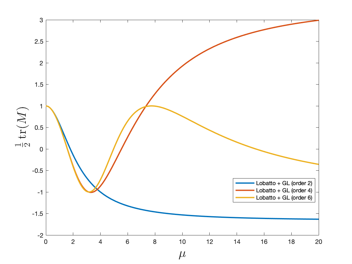
for the method of order four. The $\tilde{\mu}$ touches the line $-1$ at $\mu=2\sqrt{3}$ .

Moreover,

(46)

\tilde{\omega}h=\tilde{\mu}=\arccos\left(\frac{1-\frac{9}{20}\mu^{2}+\frac{11}{600}\mu^{4}-\frac{1}{14400}\mu^{6}}{1+\frac{1}{20}\mu^{2}+\frac{1}{600}\mu^{4}+\frac{1}{14400}\mu^{6}}\right)\qquad\mu=\omega h

for the methods of order six. The $\tilde{\mu}$ touches the line $-1$ at $\mu=\sqrt{10}$ and $1$ at $\mu=2\sqrt{15}$ .

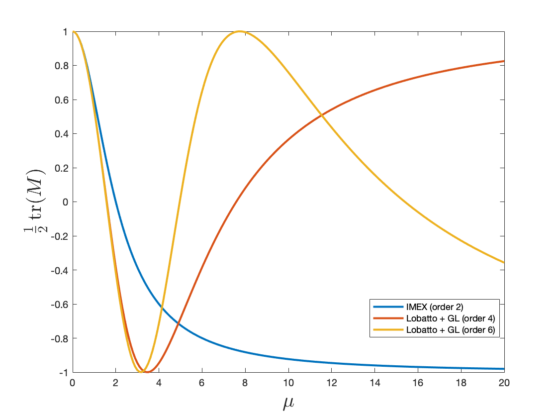
The methods $(\ref{eq:20})$ based on Lobatto IIIA-B and Gauss-Legendre of order four and six with $\tilde{A}$ by collocation $(\ref{eq:18})$ are not P-stable.

The interval of stability in the positive half plane are: $[0,4]$ for the method of order two, $[0,\frac{6}{11}\sqrt{33}]\cup[2\sqrt{3},3\sqrt{6}]$ for for the method of order four, and $[0,\sqrt{70-2\sqrt{905}}]\cup[\sqrt{10},\frac{8}{5}\sqrt{15}]\cup[2\sqrt{15},\sqrt{70+2\sqrt{905}}]$ for the methods of order six.

Proof.

The methods satisfy Lemma 4.2 therefore one has that $M_{1,1}=M_{2,2}$ . Taking either of them, the stability functions have been computed using a symbolic manipulator, as well as their points of intersections with the lines $\pm 1$ . ∎

A plot of the stability functions for the the LobattoIIIA and Gauss–Legendre combinations by interpolation $(\ref{eq:17})$ (left) and with $\tilde{A}$ by collocation $(\ref{eq:18})$ (right) for the methods of order two (IMEX), order four and order 6 is shown in Fig 1.

Refer to caption — Figure 1. *Left:* Plot of the stability functions for the the Lobatto IIIA-B and Gauss–Legendre combinations of order two (IMEX), order four and order six with coefficients constructed by interpolation $(\ref{eq:17})$ . These methods are P-stable. *Right:* Stability function plot for the methods with coefficients constructed by collocation $(\ref{eq:18})$ . For P-stability, the function must have values between $-1$ and $1$ for all $\mu$ . These methods are not P-stable. See text for their interval of stability.

5. The methods as modified trigonometric integrators

We consider the application to the test equation

(47)

\ddot{q}=-\omega^{2}q+f(q),\qquad F^{1}(q)=f(q),\quad F^{2}(q)=-\omega^{2}q.

Theorem 5.1 (Modified trigonometric integrator).

Consider the symplectic methods $(\ref{eq:17})$ applied to the test oscillatory problem $(\ref{eq:testeq})$ . Assume that the primary method has symmetric stages and that $|\frac{1}{2}\hbox{{\rm tr}}M(\mu)|\leq 1$ , with matrix $M(\mu)$ as in $(\ref{eq:Mlambda})$ having two independent eigenvectors in case of equality. Then the method can be considered as a symplectic modified trigonometric integrator with modified frequency satisfying the implicit relation

(48)

\cos(\tilde{\mu})=\frac{1}{2}\hbox{{\rm tr}}M(\mu),\qquad\tilde{\mu}=\tilde{\omega}h,\mu=\omega h

and can be written in the form

(49)

q_{1}-2\cos(\tilde{\mu})q_{0}+q_{-1}=h^{2}\psi_{1}(\tilde{\mu})(f(Q_{1})+f(Q_{-1}))+\cdots+h^{2}\psi_{s_{1}}(\tilde{\mu})(f(Q_{s_{1}})+f(Q_{-{s_{1}}})),

for $s_{1}$ implicitly defined filter functions

(50)

\psi_{i}(\tilde{\mu})=b^{T}(I_{s_{1}}+\mu^{2}\widehat{\tilde{A}}\tilde{A})^{-1}\widehat{A}_{i},\qquad\mu=\omega h,

where $\widehat{A}_{i}$ is the $i$ th column of $\widehat{A}$ . The $p$ -variables are reconstructed from the formula

(51)

2\frac{\tilde{\mu}}{\mu}\operatorname{sinc}({\tilde{\mu}})p_{0}=q_{1}-q_{-1}-h^{2}\psi_{1}(\tilde{\mu})(f(Q_{1})-f(Q_{-1}))+\cdots+h^{2}\psi_{s_{1}}(\tilde{\mu})(f(Q_{{s_{1}}})-f(Q_{-{s_{1}}})),

where the $\psi_{i}$ are the same as in $(\ref{eq:36})$ .

Proof.

As in the proof of P-stability, we ease notation and denote by capital letters $\tilde{Q}$ the vector of the internal stages $\tilde{Q}_{i}$ , by $P$ the vector of the internal momenta $P_{i}$ , by $F(Q)$ the vector of the $f(Q_{i})$ and abuse notation, to avoid the use of tensor products. Thus, the expression $b^{T}F(Q)$ means

b^{T}F(Q)=b_{1}f(Q_{1})+b_{2}f(Q_{2})+\cdots+b_{s_{1}}f(Q_{s_{1}}).

Similarly, for matrix products, the expression $\widehat{A}F(Q)$ has, as the $i$ -component, the vector $\widehat{a}_{i,1}f(Q_{1})+\cdots+\widehat{a}_{i,s_{1}}f(Q_{s_{1}})$ , etc.

Proceding as for P-stability, we see that

\begin{bmatrix}I&-h\tilde{A}\\ \omega^{2}h\widehat{\tilde{A}}&I\end{bmatrix}\begin{bmatrix}\tilde{Q}\\ P\end{bmatrix}=\begin{bmatrix}q_{0}\\ p_{0}+h\widehat{A}F(Q)\end{bmatrix}

which we use to solve for the $\tilde{Q}$ and $P$ . From $q_{1}=q_{0}+hb^{T}P$ and $p_{1}=p_{0}+hb^{T}F(Q)-h\omega^{2}\tilde{b}^{T}\tilde{Q}$ , we get

(52)		$\displaystyle\begin{bmatrix}q_{1}\\ p_{1}\end{bmatrix}$	$\displaystyle\!\!\!=\!\!\!$	$\displaystyle\begin{bmatrix}q_{0}\\ p_{0}+hb^{T}F(Q)\end{bmatrix}+h\begin{bmatrix}0&b^{T}\\ -\omega^{2}\tilde{b}^{T}&0\end{bmatrix}\begin{bmatrix}I&-h\tilde{A}\\ h\omega^{2}\widehat{\tilde{A}}&I\end{bmatrix}^{-1}\begin{bmatrix}q_{0}\\ p_{0}+h\widehat{A}F(Q)\end{bmatrix}$
(52)			$\displaystyle\!\!\!=\!\!\!$	$\displaystyle D_{\omega}M(\mu)D_{\omega}^{-1}\!\!\begin{bmatrix}q_{0}\\ p_{0}\end{bmatrix}+h\!\!\begin{bmatrix}0\\ b^{T}F(Q)\end{bmatrix}+h^{2}\!\!\begin{bmatrix}0&b^{T}\\ -\omega^{2}\tilde{b}^{T}&0\end{bmatrix}\!\!\begin{bmatrix}I&-h\tilde{A}\\ h\omega^{2}\widehat{\tilde{A}}&I\end{bmatrix}^{-1}\!\!\!\begin{bmatrix}0\\ \widehat{A}F(Q)\end{bmatrix}.$

Let $\begin{bmatrix}X_{1}&X_{2}\\ X_{3}&X_{4}\end{bmatrix}=\begin{bmatrix}I&-h\tilde{A}\\ h\omega^{2}\widehat{\tilde{A}}&I\end{bmatrix}^{-1}$ . One has

$\displaystyle X_{1}$	$\displaystyle=$	$\displaystyle(I_{s_{2}}+\mu^{2}\tilde{A}\widehat{\tilde{A}})^{-1}$
$\displaystyle X_{2}$	$\displaystyle=$	$\displaystyle h\tilde{A}(I_{s_{1}}+\mu^{2}\widehat{\tilde{A}}\tilde{A})^{-1}$
$\displaystyle X_{3}$	$\displaystyle=$	$\displaystyle-h\mu\widehat{\tilde{A}}(I_{s_{2}}+\mu^{2}\tilde{A}\widehat{\tilde{A}})^{-1}$
$\displaystyle X_{4}$	$\displaystyle=$	$\displaystyle(I_{s_{1}}+\mu^{2}\widehat{\tilde{A}}\tilde{A})^{-1}.$

Thus $q_{1}$ is given by

q_{1}=\cos(\tilde{\mu})q_{0}+h\frac{\tilde{\mu}}{\mu}\operatorname{sinc}(\tilde{\mu})p_{0}+h^{2}b^{T}(I_{s_{1}}+\mu^{2}\widehat{\tilde{A}}\tilde{A})^{-1}\widehat{A}F(Q_{+}),

where, as above, $\mu=\omega h$ and $\tilde{\mu}=\tilde{\omega}h$ is the modified frequency and $F(Q_{+})$ indicates that the internal stages are in $[0,h]$ . The $\cos(\tilde{\mu})$ and $\operatorname{sinc}(\tilde{\mu})$ terms come form $D_{\omega}M(\mu)D_{\omega^{-1}}$ in the usual way, provided that $|\frac{1}{2}M(\mu)|\leq 1$ . By replacing $h$ with $-h$ , we have

q_{-1}=\cos(\tilde{\mu})q_{0}-h\frac{\tilde{\mu}}{\mu}\operatorname{sinc}(\tilde{\mu})p_{0}+h^{2}b^{T}(I_{s_{1}}+\mu^{2}\widehat{\tilde{A}}\tilde{A})^{-1}\widehat{A}F(Q_{-}),

where, as above, $F(Q_{-})$ indicates that indicates that the internal stages are in $[0,-h]$ Taking the sum of $q_{1}$ and $q_{-1}$ , we obtain

q_{1}-2\cos(\tilde{\mu})q_{0}+q_{-1}=h^{2}b^{T}(I_{s_{1}}+\mu^{2}\widehat{\tilde{A}}\tilde{A})^{-1}\widehat{A}(F(Q_{+})+F(Q_{-})),

while subtracting the two expressions, we obtain

2h\frac{\tilde{\mu}}{\mu}\operatorname{sinc}(\tilde{\mu})p_{0}=q_{1}-q_{-1}-h^{2}b^{T}(I_{s_{1}}+\mu^{2}\widehat{\tilde{A}}\tilde{A})^{-1}\widehat{A}(F(Q_{+})-F(Q_{-})).

With some simple algebraic manipulations, it is easy to recover the filter functions. The theorem statement follows by assuming that the primary method has symmetric stages. ∎

Remark. The above theorem is also valid for all the methods described in the paper in the region where the step size $h$ is such that $|\frac{1}{2}\hbox{{\rm tr}}M|\leq 1$ .

When the first node $c_{1}=0$ then $Q_{1}=Q_{-1}=q_{0}$ so the first term on the right hand side of $(\ref{eq:29})$ becomes $2\psi_{1}(\tilde{\mu})f(q_{0})$ while it cancels in $(\ref{eq:37})$ . Moreover, in the case of the Lobatto primary method, $c_{s_{1}}=1$ hence $Q_{s_{1}}=q_{1}$ and $Q_{-s_{1}}=q_{-1}$ . However, the last column of the matrix $\widehat{A}$ is zero, and so is the last filter function $\psi_{s_{1}}$ .

For the IMEX method, we have $c_{1}=0,c_{2}=1$ ( $s_{1}=2$ ), hence $(\ref{eq:37})$ gives

2h\frac{\tilde{\mu}}{\mu}\operatorname{sinc}(\tilde{\mu})p_{0}=q_{1}-q_{-1}.

We have $\psi_{2}=0$ and

q_{1}-2\cos(\tilde{\mu})q_{0}+q_{1}=h^{2}2\psi_{1}(\tilde{\mu})f(q_{0})=h^{2}\left(1+\frac{\mu^{2}}{4}\right)^{-1}f(q_{0})

and we recover its expression as a modified trigonometric integrator

q_{1}-2\cos(\tilde{\mu})q_{0}+q_{1}=h^{2}\psi(\tilde{\mu})f(\phi(\tilde{\mu})q_{0})

with filter functions $\phi=1$ , $\psi(\xi)=\cos\xi$ satisfying the implicit relation $\cos(\tilde{\mu})=(1+\frac{\mu^{2}}{4})^{-1}$ , as derived in [MS14].

Similarly, for the order four Lobatto–Gauss-Legendre method, we have

\displaystyle 2h\frac{\tilde{\mu}}{\mu}\operatorname{sinc}(\tilde{\mu})p_{0}

\displaystyle=

\displaystyle q_{1}-q_{-1}-h^{2}\psi_{2}(\tilde{\mu})(f(q_{\frac{1}{2}})-(f(q_{-\frac{1}{2}}))

and

(53)

q_{1}-2\cos(\tilde{\mu})q_{0}+q_{-1}=h^{2}2\psi_{1}(\tilde{\mu})f(q_{0})+h^{2}\psi_{2}(\tilde{\mu})(f(q_{\frac{1}{2}})+f(q_{-\frac{1}{2}})),

with filter functions $\psi_{i}$ , $i=1,2,3$ , satisfying the implicit relations

(54)

\psi_{1}(\tilde{\mu})=\frac{2(-\mu^{2}+12)}{\mu^{4}+12\mu^{2}+144},\qquad\psi_{2}(\tilde{\mu})=\frac{2(\mu^{2}+24)}{\mu^{4}+12\mu^{2}+144},\qquad\psi_{3}=0

( $\phi_{i}=1$ , $i=1,2,3$ ). The modified frequency is given by $(\ref{eq:35})$ .

Finally, for the of order 6 Lobatto–Gauss-Legendre method, we have similar expressions, with filters implicitly defined by

(55)

\begin{array}[]{rcl}\psi_{1}(\tilde{\mu})&=&\frac{2\mu^{4}-140\mu^{2}+1200}{\mu^{6}+24\mu^{4}+720\mu^{2}+14400},\\ \psi_{2}(\tilde{\mu})&=&\frac{-(\mu^{4}+50\mu^{2}-600)\sqrt{5}-50\mu^{2}+3000}{\mu^{6}+24\mu^{4}+720\mu^{2}+14400},\\ \psi_{3}(\tilde{\mu})&=&\frac{(\mu^{4}+50\mu^{2}-600)\sqrt{5}-50\mu^{2}+3000}{\mu^{6}+24\mu^{4}+720\mu^{2}+14400},\\ \psi_{4}(\tilde{\mu})&=&0,\end{array}

and modified frequency given by $(\ref{eq:50})$ .

6. Numerical experiments

As a bed test, we consider the Fermi-Pasta-Ulam-Tsingou (FPUT, formerly FPU) problem of alternating soft and stiff springs, that has been extensively used in literature to study methods for oscillatory problems. Because of the oscillatory nature of the problem, among all the methods proposed, we test only those that are P-stable, as methods that are not P-stable are likely to produce diverging solution as soon as the step size leaves the region of P-stability. Therefore, in what follows, all the numerical experiments are performed with the Lobatto–Gauss-Legendre family $(\ref{eq:20})$ with coefficients by interpolation $(\ref{eq:18})$ . We will compare these methods also with higher order integrators obtained using the IMEX (wich is the Lobatto–Gauss-Legendre method of order 2) and the Yoshida time stepping technique.

6.1. The Fermi-Pasta-Ulam-Tsingou problem

For comparison with [EH06, MS14], we consider the same setup with $2\ell$ points of unit mass representing alternating soft nonlinear springs and stiff linear springs. Setting $q$ to be the concatenation of slow (index $s$ ) and fast (index $f$ ) position variables,

q=[q_{s,1},\ldots,q_{s,\ell},q_{f,1},\ldots,q_{f,\ell}]^{T},

and $p$ the corresponding momenta, the Hamiltonian reads

\begin{split}H(q,p)&=\frac{1}{2}\sum_{i=1}^{\ell}(p_{s,i}^{2}+p_{f,i}^{2})+\frac{\omega^{2}}{2}\sum_{i=1}^{\ell}q_{f,i}^{2}\\ &\qquad+\frac{1}{4}\left[(q_{s,1}-q_{f,1})^{4}+\sum_{i=1}^{\ell-1}(q_{s,i+1}-q_{f,i+1}-q_{s,i}-q_{f,i})^{4}+(q_{s,\ell}+q_{f,\ell})^{4}\right].\end{split}

In our setup, the nonlinear potential and kinetic energy are treated with the Lobatto IIIA-B pair, while the linear stiff energy $\frac{\omega^{2}}{2}\sum_{i=1}^{\ell}q_{f,i}^{2}$ is treated with the Gauss–Legendre methods based on interpolation.

The total oscillatory energy $I$ ,

I(q_{f},p_{f})=\frac{1}{2}\sum_{i=1}^{\ell}p_{f,i}^{2}+\frac{\omega^{2}}{2}\sum_{i=1}^{\ell}q_{f,i}^{2}=I_{1}+\ldots+I_{\ell}

is defined as the sum of the oscillatory energies of each fast spring. For ease of comparison with the numerical examples in literature, the initial conditions used in the simulations are the same as those in [EH06, MS14]

q_{s,1}(0)=1,\quad p_{s,1}(0)=1,\quad q_{f,1}(0)=\omega^{-1},\quad p_{f,1}(0)=1,

and all the other initial values equal to zero. In the numerical experiments, we use $\ell=3$ .

The left plot in figure $(\ref{fig:OsciHerr})$ shows the oscillatory energies for each spring and the total oscillatory energy, comparing the IMEX method (which is the lowest method in the class) and the higher order proposed method based interpolation (Lobatto–Gauss-Legendre of order 4 and 6). The right plot shows the corresponding error in the Hamiltonian energy.

When the modified frequency $\tilde{\omega}$ is such that $\cos(h\tilde{\omega})=\pm 1$ , see Figure 1, left plot, we expect to observe resonances. This happens for $h\omega/\pi=2\sqrt{3}/\pi\approx 1.1$ for order four method and for $h\omega/\pi=\sqrt{10}/\pi\approx 1$ and $h\omega/\pi=2\sqrt{15}/\pi\approx 2.47$ for the order six method. Resonances can be observed in the preservation of the Hamiltonian (total) energy of the system and in the scaled total oscillatory energy $\omega I$ in the range $(0,4.5\pi]$ , the latter being more uniform in dealing with the frequencies. It is clear that the width of the resonance region is inversely propotional to the curvature at the resonance point. The flatter the stability function is at the resonance points in Figure reffig:Mlambda, the wider the region of resonance.

The left plot in Figure 5 displays the solution obtained by the methods by taking a relatively large step size, with $h\omega/\pi\approx 1.59$ . The approximations to the solutions are still fairly acceptable and the methods do not display excessive oscillations as other trigonometric integrators do.

The right plot in Figure 5 depicts the behavior of the methods as they approach their high-frequency limit, in a similar experiment as in [MS14]. We keep $h=0.1$ but take $\omega=1000$ with a ratio $h\omega/\pi\approx 31.8$ . In this experiment $\omega$ is scaled by a factor of $20$ (compared to 200 in [MS14]) and the time interval must also be scaled correspondingly to $[0,4000]$ .

A rough analysis of the slow energy exchange can be performed by using the modified trigonometric integrator form of the method and the expansion of the exact and numerical solution using modulate Fourier expansions, see [EH06, MS14]. One difficulty with respect to the standard analysis using modified trigonometric integrators is the presence of more filter functions $\psi$ in $(\ref{eq:29})$ and of the internal stages of the methods. However, performing a Taylor expansion of the internal stages, one can put the methods in the form

q_{1}-2\cos(\tilde{\mu})q_{0}+q_{-1}=h^{2}\psi(\tilde{\mu})f(\phi(\tilde{\mu})q_{0})+\mathcal{O}(h^{4})

and apply the standard analysis as for trigonometric integrators.

For instance, for the Lobatto–Gauss-Legendre method of order 4, one has that $\phi=1$ , $\psi(\tilde{\mu})=2(\psi_{1}(\tilde{\mu})+\psi_{2}(\tilde{\mu}))=1/(1+\frac{1}{12}\mu^{2}+\frac{1}{144}\mu^{4})$ , with $\mu=h\omega$ (the $\psi$ -functions are defined implicitly).

Using the same setup as in [EH06, MS14], one finds that $\alpha=1+\frac{1}{6}\mu^{2}+\mathcal{O}(\mu^{4})$ , $\beta=1$ , and $\gamma=1-\frac{1}{1728}\mu^{6}+\mathcal{O}(\mu^{8})$ . In order to preserve the slow energy exchange at a correct rate, it is required that $\alpha=\beta=\gamma=1$ , a property that is satisfied only by the IMEX, as proven in [MS14]. It is in particular the value of $\alpha$ that has the strongest effect on the slow energy exchange. Nevertheless, the methods perform way better than classical trigonometric integrators.

Figure 6 shows the Hamiltonian maximum error ratio computed for $h=0.04$ and $h=0.02$ for various values of $\omega$ up to $4.5\pi$ . In the convergence region we would expect that the ratio would be $16$ for the method of order $4$ and $64$ for the method of order $6$ , however the plot does not cover well the convergence region. Overall, we see that the methods have a conservation of $\mathcal{O}(h^{2})$ , except from the regions corresponding to resonances. This behaviour seems to indicate that the methods suffer of order reduction, a phenomenon that is not uncommon for higher order methods in prescribed regions of the step-size. This effect will be discussed more thoroughly below.

6.2. Order reduction

Ultimately, it is the error in the slow variables one of the most relevant quantities in the numerical simulations of these kind of problems, because the fast variables will be in any case poorly resolved. In figures (7–8) we show the errors in the slow variables for the FPUT problem for different values of the step-size and different $\omega$ . The errors are evaluated at $T=3$ and the exact solution is computed using Matlab’s ode45 to about machine precision (setting AbsTol, RelTol = 1e-14). It is observed that the methods suffer of order reduction both in the positions and the momenta, manifested as a platou in the error plots.

In figures (9)-(10) we repeat the same experiments by methods of order 4 and 6 obtained from the IMEX and using the Yoshida technique [Yos90]. Also in this case one can observe an order reduction, from order 4 to order 3 for the positions and from order 4 to 2 for the momenta for the method of order 4. Similarly, one observes a reduction from order 6 to order 3 for the positions and from order 6 to order 2 for the momenta for the method of order 6. In summary, the order reduction is similar to that of the Lobatto–Gauss-Legendre on the momenta, but is one order less on the positions.

It is not clear why the Yoshida technique gives a lesser order reduction for the positions and marginally also for the momenta. We conjecture that it might be due to the fact that the method uses step sizes $\alpha h$ and $\beta h$ , rather than just $h$ , and the use of these two step sizes might reduce the resonance effects of the single step size.

Figures (11)-(12) show a comparison of the errors for methods of the same order. It is observed that for larger step-sizes, the Lobatto–Gauss-Legendre have smaller error (about two orders of magnitude) than IMEX with Yoshida timestepping. For smaller step-sizes, there is no obvious answer and the choice of the method will most likely depend on the application under consideration.

The Lobatto–Gauss-Legendre of order 4 and 6 have implicit stages, which require one and two functions evaluations respectively. In our numerical experiments, we have solved the implicit stages by fixed point iteration. The number of function evaluations will then depend on the number of fixed point iterations. For small step sizes, we observed 1-2 fixed point iterations. For larger step sizes (but still in the convergence region) we never observed more than 10 iterations, a typical number was $\approx$ 5-6. In comparison, the order 4 IMEX with the Yoshida technique would require 3 function evaluations and 9 function evaluation for order 6. However, the Yoshida techniques have larger error in the regions of convergence, especially in the larger step size regions. This error is about two-three orders of magnitude larger than the Lobatto–Gauss-Legendre methods, indicating that these can be used with a larger step size, resulting in an overall cheaper method.

7. Conclusions and further remarks

We have introduced a family of symplectic methods based on a variational derivation. The main idea is to use different integration quadrature formulas for different terms of the Lagrangian. The introduction of extra internal stages is solved either by interpolation or by collocation. In particular, we have derived a higher order generalization of the IMEX method (using the Verlet method and an interpolated form of the Implicit Midpoint Rule), namely the LobattoIIIA-B–Gauss-Legendre family of arbitrary order, and present the coefficients explicitly for the methods of order 4 and 6. We have proved that these method possess the expected order and shown that the methods with internal stages solved by interpolation are P-stable, making these particularly interesting in the context of oscillatory problem. We have also observed that these higher order methods might suffer from resonance and from order reduction. The methods are thoroughly tested on the FPUT problem and their behaviour is compared to higher order IMEX implementations using the Yoshida time-stepping technique.

The proposed methods might be considered as special subclass of additive Runge–Kutta methods (ARK). The advantage of the variational derivation is that the methods are automatically symplectic, therefore particularly suited to geometric integration. It will be interesting to explore further this mixed technique for other choices of primary/secondary methods and the use other techniques, like treating some of the terms by averaged Lagrangian methods in the spirit of [CH17]. Possibly, this mixed approach might lead to further interesting numerical method that might not be easily discovered using the classical algebraic theory of RK and ARK methods.

Acknowledgements

The author would like to thank MSc Fredrick Pfeil for some very preliminary results and simulations for the FPUT problem [Pfe19]. The final part of this work was completed at the Isaac Newton Institute for Mathematical Sciences, which the author acknowledges for support and hospitality during the programme Geometry, compatibility and structure preservation in computational differential equations (2019), EPSRC grant number EP/R014604/1. This work was also partially supported by European Union Horizon 2020 research and innovation programme under the Marie Sklodowska-Curie grant agreement No. 691070, Challeges in preservation of structure (CHiPS).

Appendix A The family of Lobatto IIIA-IIIB (primary) and Gauss-Legendre (secondary) methods

A.1. Methods based on interpolation

A.1.1. The IMEX

We consider the case the primary method for $L^{1}$ is the trapezoidal rule, giving rise to the Verlet scheme, a Lobatto IIIA-IIIB pair PRK with coefficients $(A,b,c)$ and $(\widehat{A},b,c)$

\begin{array}[]{c|cc}0&0&0\\ 1&\frac{1}{2}&\frac{1}{2}\\[2.0pt] \hline\cr\\[-12.0pt] &\frac{1}{2}&\frac{1}{2}\end{array},\qquad\begin{array}[]{c|cc}0&\frac{1}{2}&0\\ 1&\frac{1}{2}&0\\[2.0pt] \hline\cr\\[-12.0pt] &\frac{1}{2}&\frac{1}{2}\end{array}.

The secondary scheme is the IMR ( $s_{2}=1$ , $\tilde{c}_{1}=\frac{1}{2}$ , $\tilde{b}_{1}=1$ ). One has

\tilde{A}=\begin{bmatrix}\tilde{a}_{1,1}&\tilde{a}_{1,2}\end{bmatrix}=\begin{bmatrix}\frac{1}{4}&\frac{1}{4}\end{bmatrix},\qquad\widehat{\tilde{A}}=\begin{bmatrix}\frac{1}{2}\\[5.0pt] \frac{1}{2}\end{bmatrix}

A.1.2. Method of order four

To construct higher order methods we look at the Lobatto IIIA-IIIB pair ( $s=3$ ) and GL ( $s=2$ ).

A=\begin{bmatrix}0&0&0\\ \vskip 6.0pt plus 2.0pt minus 2.0pt\cr\frac{5}{24}&\frac{1}{3}&-\frac{1}{24}\\ \vskip 6.0pt plus 2.0pt minus 2.0pt\cr\frac{1}{6}&\frac{2}{3}&\frac{1}{6}\end{bmatrix}\qquad\widehat{A}=\begin{bmatrix}\frac{1}{6}&-\frac{1}{6}&0\\ \vskip 6.0pt plus 2.0pt minus 2.0pt\cr\frac{1}{6}&\frac{1}{3}&0\\ \vskip 6.0pt plus 2.0pt minus 2.0pt\cr\frac{1}{6}&\frac{5}{6}&0\end{bmatrix},

with

c=\begin{bmatrix}0&\frac{1}{2}&1\end{bmatrix}^{T},\qquad b=\begin{bmatrix}\frac{1}{6}&\frac{2}{3}&\frac{1}{6}\end{bmatrix}^{T}.

For the Gauss-Legendre quadrature, we have

\tilde{c}=\begin{bmatrix}\frac{1}{2}-\frac{\sqrt{3}}{6}&\frac{1}{2}+\frac{\sqrt{3}}{6}\end{bmatrix}^{T},\qquad\tilde{b}=\begin{bmatrix}\frac{1}{2}&\frac{1}{2}\end{bmatrix}^{T}.

We consider the interpolation case $(\ref{eq:18})$ . The matrix $\tilde{A}$ and $\widehat{\tilde{A}}$ are

\tilde{A}=\begin{bmatrix}\frac{1}{6}-\frac{\sqrt{3}}{36}&\frac{1}{3}-\frac{\sqrt{3}}{9}&-\frac{\sqrt{3}}{36}\\ \vskip 6.0pt plus 2.0pt minus 2.0pt\cr\frac{1}{6}+\frac{\sqrt{3}}{36}&\frac{1}{3}+\frac{\sqrt{3}}{9}&\frac{\sqrt{3}}{36}\end{bmatrix},\qquad\widehat{\tilde{A}}=\begin{bmatrix}\frac{\sqrt{3}}{12}&-\frac{\sqrt{3}}{12}\\ \vskip 6.0pt plus 2.0pt minus 2.0pt\cr\frac{1}{4}+\frac{\sqrt{3}}{12}&\frac{1}{4}-\frac{\sqrt{3}}{12}\\ \vskip 6.0pt plus 2.0pt minus 2.0pt\cr\frac{1}{2}+\frac{\sqrt{3}}{12}&\frac{1}{2}-\frac{\sqrt{3}}{12}\end{bmatrix}

As for the primary method, we have $Q_{1}=q_{0}$ and $Q_{3}=q_{1}$ .

A.1.3. Method of order six

Consider the Lobatto IIIA-IIIB pair ( $s=4$ ) and GL ( $s=3$ ),

A=\begin{bmatrix}0&0&0&0\\ \frac{11+\sqrt{5}}{120}&\frac{25-\sqrt{5}}{120}&\frac{25-13\sqrt{5}}{120}&\frac{-1+\sqrt{5}}{120}\\ \vskip 6.0pt plus 2.0pt minus 2.0pt\cr\frac{11-\sqrt{5}}{120}&\frac{25+13\sqrt{5}}{120}&\frac{25+\sqrt{5}}{120}&\frac{-1-\sqrt{5}}{120}\\ \vskip 6.0pt plus 2.0pt minus 2.0pt\cr\frac{1}{12}&\frac{5}{12}&\frac{5}{12}&\frac{1}{12}\end{bmatrix},\qquad\widehat{A}=\begin{bmatrix}\frac{1}{12}&\frac{-1-\sqrt{5}}{24}&\frac{-1+\sqrt{5}}{24}&0\\ \vskip 6.0pt plus 2.0pt minus 2.0pt\cr\frac{1}{12}&\frac{25+\sqrt{5}}{120}&\frac{25-13\sqrt{5}}{120}&0\\ \vskip 6.0pt plus 2.0pt minus 2.0pt\cr\frac{1}{12}&\frac{25+13\sqrt{5}}{120}&\frac{25-\sqrt{5}}{120}&0\\ \vskip 6.0pt plus 2.0pt minus 2.0pt\cr\frac{1}{12}&\frac{11-\sqrt{5}}{24}&\frac{11+\sqrt{5}}{24}&0\\ \end{bmatrix}

with

c=\begin{bmatrix}0&\frac{1}{2}-\frac{\sqrt{5}}{10}&\frac{1}{2}+\frac{\sqrt{5}}{10}&1\end{bmatrix}^{T},\qquad b=\begin{bmatrix}\frac{1}{12}&\frac{5}{12}&\frac{5}{12}&\frac{1}{12}\end{bmatrix}^{T}.

For the Gauss-Legendre quadrature, we have

\tilde{c}=\begin{bmatrix}\frac{1}{2}-\frac{\sqrt{15}}{10}&\frac{1}{2}&\frac{1}{2}+\frac{\sqrt{15}}{10}\end{bmatrix}^{T},\qquad\tilde{b}=\begin{bmatrix}\frac{5}{18}&\frac{4}{9}&\frac{5}{18}\end{bmatrix}^{T}.

We consider the interpolation case $(\ref{eq:18})$ . The matrix $\tilde{A}$ and $\widehat{\tilde{A}}$ are

\tilde{A}=\begin{bmatrix}\frac{1}{15}&{\frac{25-6\sqrt{15}+3\sqrt{5}}{120}}&{\frac{25-6\sqrt{15}-3\sqrt{5}}{120}}&{\frac{1}{60}}\\ \vskip 6.0pt plus 2.0pt minus 2.0pt\cr{\frac{5}{48}}&{\frac{5}{24}}+\frac{\sqrt{5}}{16}&{\frac{5}{24}}-\frac{\sqrt{5}}{16}&-\frac{1}{48}\\ \vskip 6.0pt plus 2.0pt minus 2.0pt\cr\frac{1}{15}&{\frac{25+6\sqrt{15}+3\sqrt{5}}{120}}&{\frac{25+6\sqrt{15}-3\sqrt{5}}{120}}&{\frac{1}{60}}\end{bmatrix}\qquad\widehat{\tilde{A}}=\begin{bmatrix}\frac{1}{18}&-\frac{1}{9}&\frac{1}{18}\\ \vskip 6.0pt plus 2.0pt minus 2.0pt\cr{\frac{25+6\sqrt{15}-3\sqrt{5}}{180}}&\frac{2}{9}-\frac{\sqrt{5}}{15}&{\frac{25-6\sqrt{15}-3\sqrt{5}}{180}}\\ \vskip 6.0pt plus 2.0pt minus 2.0pt\cr{\frac{25+6\sqrt{15}+3\sqrt{5}}{180}}&\frac{2}{9}+\frac{\sqrt{5}}{15}&{\frac{25-6\sqrt{15}+3\sqrt{5}}{180}}\\ \vskip 6.0pt plus 2.0pt minus 2.0pt\cr\frac{2}{9}&\frac{5}{9}&\frac{2}{9}\par\end{bmatrix}

A.2. Methods based on collocation

The weights $b,\tilde{b}$ and nodes $c,\tilde{c}$ of the primary and secondary method of each order, as well as the correspoding PRK for the primary methods are the same as for interpolation. The difference is in the coefficient matrices $\tilde{A}$ and $\widehat{\tilde{A}}$ , which we report below for convenience.

A.2.1. Second order method

\tilde{A}=\begin{bmatrix}\frac{3}{8}&\frac{1}{8}\end{bmatrix},\qquad\widehat{\tilde{A}}=\begin{bmatrix}\frac{1}{4}\\[5.0pt] \frac{3}{4}\end{bmatrix}.

A.2.2. Fourth order method

\tilde{A}=\begin{bmatrix}\frac{1}{6}-{\frac{\sqrt{3}}{108}}&\frac{1}{3}-{\frac{4\sqrt{3}}{27}}&-{\frac{\sqrt{3}}{108}}\\ \vskip 6.0pt plus 2.0pt minus 2.0pt\cr\frac{1}{6}+{\frac{\sqrt{3}}{108}}&\frac{1}{3}+{\frac{4\sqrt{3}}{27}}&{\frac{\sqrt{3}}{108}}\end{bmatrix},\qquad\widehat{\tilde{A}}=\begin{bmatrix}\frac{\sqrt{3}}{36}&-\frac{\sqrt{3}}{36}\\ \vskip 6.0pt plus 2.0pt minus 2.0pt\cr\frac{1}{4}+\frac{\sqrt{3}}{9}&\frac{1}{4}-\frac{\sqrt{3}}{9}\\ \vskip 6.0pt plus 2.0pt minus 2.0pt\cr\frac{1}{2}+\frac{\sqrt{3}}{36}&\frac{1}{2}-\frac{\sqrt{3}}{36}\end{bmatrix}.

A.2.3. Six order method

\tilde{A}=\begin{bmatrix}{\frac{19}{240}}&{\frac{\sqrt{5}\left(\sqrt{15}-5\right)^{2}\left(3\,\sqrt{15}+4\,\sqrt{5}+2\,\sqrt{3}+12\right)}{2400}}&-{\frac{\sqrt{5}\left(\sqrt{15}-5\right)^{2}\left(3\,\sqrt{15}-2\,\sqrt{3}-4\,\sqrt{5}+12\right)}{2400}}&{\frac{1}{240}}\\ \vskip 6.0pt plus 2.0pt minus 2.0pt\cr{\frac{17}{192}}&{\frac{5}{24}}+{\frac{5\,\sqrt{5}}{64}}&{\frac{5}{24}}-{\frac{5\,\sqrt{5}}{64}}&-{\frac{1}{192}}\\ \vskip 6.0pt plus 2.0pt minus 2.0pt\cr{\frac{19}{240}}&-{\frac{\sqrt{5}\left(\sqrt{15}+5\right)^{2}\left(3\,\sqrt{15}-4\,\sqrt{5}+2\,\sqrt{3}-12\right)}{2400}}&{\frac{\sqrt{5}\left(\sqrt{15}+5\right)^{2}\left(3\,\sqrt{15}+4\,\sqrt{5}-2\,\sqrt{3}-12\right)}{2400}}&{\frac{1}{240}}\end{bmatrix},

\widehat{\tilde{A}}=\begin{bmatrix}{\frac{1}{72}}&-\frac{1}{36}&{\frac{1}{72}}\\ \vskip 6.0pt plus 2.0pt minus 2.0pt\cr{\frac{5}{36}}+{\frac{\left(12\,\sqrt{3}-3\right)\sqrt{5}}{360}}&\frac{2}{9}-\frac{\sqrt{5}}{12}&{\frac{5}{36}}+{\frac{\left(-12\,\sqrt{3}-3\right)\sqrt{5}}{360}}\\ \vskip 6.0pt plus 2.0pt minus 2.0pt\cr{\frac{5}{36}}+{\frac{\left(12\,\sqrt{3}+3\right)\sqrt{5}}{360}}&\frac{2}{9}+\frac{\sqrt{5}}{12}&{\frac{5}{36}}+{\frac{\left(-12\,\sqrt{3}+3\right)\sqrt{5}}{360}}\\ \vskip 6.0pt plus 2.0pt minus 2.0pt\cr{\frac{19}{72}}&{\frac{17}{36}}&{\frac{19}{72}}\par\end{bmatrix}.

References

[CH17] E. Celledoni and E. H. Høyseth. The averaged Lagrangian method. J. Comp. Appl. Math., 316:161–174, 2017.
[CS83] G. J. Cooper and A. Sayfy. Additive Runge–Kutta methods for stiff ordinary differential equations. Math. Comp., 40(161):207–2018, 1983.
[EH06] G. Wanner E. Hairer, C. Lubich. Geometric Numerical Integrtion, Structure-Preserving Algorithms for Ordinary Differential Equations. Springer Series in Computational Mathematics. Springer, 2006.
[Jay98] L. Jay. Structure preservation for constrained dynamics with super partitioned additive Runge–Kutta methods. SIAM J. Sci. Comput., 20(2):416–446, 1998.
[JP95] L. O. Jay and L. R. Petzold. Highly oscillatory systems and periodc stability. Technical Report 95-015, Army High Performance Computing Research Center, Stanford, CA, 1995.
[MS14] R. I. McLachlan and A. Stern. Modified trigonometric integrators. SIAM J. Numer. Anal., 52(3):1378–1397, 2014.
[MST11] R. I. McLachlan, Y. Sun, and P. S. P. Tse. Linear stability of partitioned Runge-Kutta methods. SIAM J. Num. Anal., 49(1):232–263, 2011.
[MW01] J. E. Marsden and M. West. Discrete mechanics and variational integrators. Acta Numerica, 10:357–514, 2001.
[Pfe19] F. Pfeil. A higher order IMEX method for solving highly oscillatory problems. Master’s thesis, University of Bergen, Norway, June 2019.
[SG09] Ari Stern and Eitan Grinspun. Implicit-explicit variational integration of highly oscillatory problems. Multiscale Model. Simul., 7(4):1779–1794, 2009.
[SG15] A. Sandu and M. Günther. A generalized-structure approach to additive Runge–Kutta methods. SIAM J. Num. Anal., 53(1):17–42, 2015.
[Tan18] G. M. Tanner. Generalized additive Runge–Kutta methods for stiff ODEs. PhD thesis, University of Iowa, 2018.
[WOBL16] T. Wenger, S. Ober-Blöbaum, and S. Leyendecker. Variational integrators of mixed order for dynamical systems with multiple time scales and split potentials. In G. Stefanou M. Papadrakakis, V. Papadopoulos and V. Plevris, editors, ECCOMAS Congress 2016, 2016.
[WOBL17] T. Wenger, S. Ober-Blöbaum, and S. Leyendecker. Construction and analysis of higher order variational integrators for dynamical systems with holonomic constraints. Advances in Computational Mathematics, 43(5):1163–1195, Oct 2017.
[Yos90] H. Yoshida. Construction of higher order symplectic integrators. Physics Letters A, 150:262–268, 1990.
[Zan17] A. Zanna. A family of modified trigonometric integrators for highly oscillatory problems. FoCM, Barcelona, 2017.
[ZS97] M. Zhang and R. D. Skeel. Cheap implicit symplectic integrators. Appl. Num. Math., 25:297–302, 1997.

Symplectic P-stable Additive Runge–Kutta MethodsThanks: † Matematisk institutt, Universitetet i Bergen, Norway, email: Antonella.Zanna@uib.no

Abstract.

1. Introduction

2. Variational derivation

2.1. General format of the methods

Theorem 2.1.

Proof.

2.2. Construction of the matrix A~\tilde{A}

3. Order of the methods

Lemma 3.1.

Proof.

Theorem 3.2.

Proof.

Corollary 3.2.1.

4. P-stability

Definition 4.1.

Theorem 4.1.

Proof.

Corollary 4.1.1.

Proof.

Lemma 4.2.

Proof.

Theorem 4.3.

Proof.

5. The methods as modified trigonometric integrators

Theorem 5.1 (Modified trigonometric integrator).

Proof.

6. Numerical experiments

6.1. The Fermi-Pasta-Ulam-Tsingou problem

6.2. Order reduction

7. Conclusions and further remarks

Acknowledgements

Appendix A The family of Lobatto IIIA-IIIB (primary) and Gauss-Legendre (secondary) methods

A.1. Methods based on interpolation

A.1.1. The IMEX

A.1.2. Method of order four

A.1.3. Method of order six

A.2. Methods based on collocation

A.2.1. Second order method

A.2.2. Fourth order method

A.2.3. Six order method

References

Symplectic P-stable Additive Runge–Kutta MethodsThanks: ^† Matematisk institutt, Universitetet i Bergen, Norway, email: Antonella.Zanna@uib.no

2.2. Construction of the matrix $\tilde{A}$