Faster saddle-point optimization for solving
large-scale Markov decision processes

Computing optimal policies in Markov decision processes (MDPs) is one of the most important problems in sequential decision making and control (Puterman 1994). Arguably, the most classical approach to solve this task is through the method of dynamic programming, understood in this context as computing fixed points of certain operators (Bellman 1957; Howard 1960; Bertsekas 2007). The use and influence of dynamic-programming methods like value and policy iteration extend well beyond the world of decision and control theory, as the underlying ideas serve as foundations for most algorithms for learning optimal policies in unknown MDPs: the setting of reinforcement learning (Szepesvári 2010; Sutton and Barto 2018). While being hugely successful, DP-based methods have the downside of being somewhat incompatible with classical machine-learning tools that are rooted in convex optimization. Indeed, most of the popular reductions of dynamic programming to (non-)convex optimization are based on heuristics that are not directly motivated by theory. Examples include the celebrated DQN approach of Mnih et al. 2015 that reduces value-function estimation to minimizing the “squared Bellman error”, or the TRPO algorithm of Schulman et al. 2015 that reduces policy updates to minimizing a “regularized surrogate objective”. While these methods can be justified to a certain extent, it is technically unknown if solving the resulting optimization problems actually leads to a desirable solution to the original sequential decision-making problem.

In this paper, we explore a family of methods that reduce MDP optimization to a form of convex optimization in a theoretically grounded way. Our starting point is an alternative approach based on linear programming (LP), first proposed roughly at the same time as the DP methods of Bellman 1957; Howard 1960: the idea of LP-based methods for sequential decision-making goes back to the works of de Ghellinck 1960; Manne 1960; Denardo 1970. While LP-based methods seem to be more obscure in present day than DP methods, they have the clear advantage that they lead to an objective function directly amenable to modern large-scale optimization methods. Recent reinforcement-learning methods inspired by the LP perspective include policy-gradient and actor-critic methods (Sutton et al. 1999; Konda and Tsitsiklis 1999) and various “entropy-regularized” learning algorithms (e.g., Peters et al. 2010; Zimin and Neu 2013; Neu et al. 2017). While these methods promise to directly tackle the policy-optimization problem through solving the underlying linear program, most of them still require the computation of certain value functions through dynamic programming.

In the present work, we argue for the viability of a method fully based on a form of convex optimization, rooted in the LP approach. Our approach is based on a bilinear saddle-point formulation of the linear program, building on a well-known general equivalence between the two optimization problems. One particular advantage of this formulation is that it enables a straightforward form of dimensionality reduction of the original problem through a linear parametrization of the optimization variables, which provides a natural framework for studying effects of “function approximation” in the underlying policy optimization problem. Our main contribution regarding this setting lies in characterizing a set of assumptions that allow a reduced-order saddle-point representation of the optimal policy. These include a realizability assumption and a newly identified coherence assumption about the subspaces used for approximation. Our main positive result is showing that these conditions are sufficient for constructing an algorithm that outputs an $\varepsilon$-optimal policy with runtime guarantees of $\widetilde{\mathcal{O}}\left(\tau_{\mbox{\scriptsize{mix}}}^{2}N^{3}/\varepsilon\right)$, where $N$ is the number of variables in the relaxed optimization problem, and $\tau_{\mbox{\scriptsize{mix}}}$ is a notion of mixing time. Our approach is based on the celebrated Mirror Prox algorithm of Nemirovski 2004 (see also Korpelevich 1976). We complement our positive results by showing that our newly defined coherence assumption is necessary for the relaxed saddle-point approach to be viable: we construct a simple example violating the assumption, where achieving full optimality on the relaxed problem leads to a suboptimal policy.

We are not the first to consider saddle-point methods for optimization in Markov decision processes. Wang 2017 proposed variants of Mirror Descent to solve the original saddle-point problem without relaxations and provide runtime guarantees of $\widetilde{\mathcal{O}}\bigl(\left(\alpha\tau_{\mbox{\scriptsize{mix}}}\right)^{2}|\mathcal{X}||\mathcal{A}|/\varepsilon^{2}\bigr)$, where $\mathcal{X}$ and $\mathcal{A}$ are the finite state and action spaces, and $\alpha$ is a parameter that characterizes the uniformity of the stationary distributions of every policy. Specifically, their assumption implies¹¹ 1 The actual assumption made by Wang 2017 is even more restrictive. that for the stationary distribution $d_{\pi}$ any policy $\pi$, one has $\frac{\max_{x}d_{\pi}(x)}{\min_{x^{\prime}}d_{\pi}(x^{\prime})}\leq\alpha$. In most cases of practical interest, this ratio is at least as large as $|\mathcal{X}|$ (e.g., when there are states that some policies visit with constant probability), and can easily be exponentially large in $|\mathcal{X}|$, or even infinite if the underlying MDP has transient states. When specialized to this setting, our bounds replace $\alpha^{2}$ by the much more manageable $|\mathcal{X}|$ and also improve the dependence on $\varepsilon$ from $1/\varepsilon^{2}$ to $1/\varepsilon$. One downside of our method is that we need full access to the transition probabilities of the MDP, whereas the algorithm of Wang 2017 only requires a generative model.

The linearly relaxed saddle-point problem we consider was first studied by Lakshminarayanan et al. 2018 and Chen et al. 2018. Our runtime guarantees improve over the ones claimed by Chen et al. 2018 in a similar way as our first set of results improve over those of Wang 2017. Notably, their results still feature a factor of $\alpha^{2}$, which generally depends on the size of the original state space rather than the number of features, rendering these guarantees void of meaning in very large state spaces. In contrast, our bounds replace this factor by the number of features $N$. Furthermore, our characterization highlighting the importance of the coherence assumption discussed above hints at some potential technical issues with the results of Chen et al. 2018, who claimed convergence to the optimal policy without the coherence assumption.

The rest of the paper is organized as follows. After providing background on the saddle-point formulation of MDP optimization in Section 2, we describe the relaxed saddle-point problem in Section 3. Section 4 presents our algorithm and its performance guarantees, and Section 5 provides a sketch of the proofs. We conclude by providing a simple numerical illustration of our method in Section 6 and discuss our results in Section 7.

Consider an undiscounted Markov decision process $M=(\mathcal{X},\mathcal{A},P,r)$, where $\mathcal{X}$ is the finite state space, $\mathcal{A}$ is the finite action space, $P$ is the transition function with $P(x^{\prime}|x,a)$ denoting the probability of moving to state $x^{\prime}\in\mathcal{X}$ from state $x\in\mathcal{X}$ when taking action $a\in\mathcal{A}$ and $r$ is the reward function mapping state-action pairs to rewards with $r(x,a)$ denoting the reward of being in state $x$ and taking action $a$. We assume that $r(x,a)\in[0,1]$ for all $x,a$. In each round $t$, the learner observes state $x_{t}\in\mathcal{X}$, selects action $a_{t}\in\mathcal{A}$, moves to the next state $x_{t+1}\sim P(\cdot|x_{t},a_{t})$, and obtains reward $r(x_{t},a_{t})$.

In this paper we focus on the infinite-horizon average-reward scenario where the goal of the learner is to select its actions $a_{t}$ in a way that maximizes the average reward per time step, $\lim\inf_{t\rightarrow\infty}\mathbb{E}\left[\frac{1}{T}\sum_{t=1}^{T}r_{t}(x_{t},a_{t})\right]$. We will work with randomized stationary policies with $\pi(a|x)$ denoting the probability of taking action $a$ in state $x$. Under technical assumptions discussed shortly, each such policy $\pi$ generates a unique stationary state distribution $d_{\pi}\in\Delta_{\mathcal{X}}$ over the state space satisfying $d_{\pi}(x)=\lim_{t\rightarrow\infty}\mathbb{P}\left[x_{t}=x\right]$ for all $x$ when the trajectory $(x_{t})_{t}$ is generated by following policy $\pi$. Similarly, each policy $\pi$ generates a stationary state-action distribution $\mu_{\pi}\in\Delta_{\mathcal{X}\times\mathcal{A}}$ satisfying $\mu_{\pi}(x,a)=\lim_{t\rightarrow\infty}\mathbb{P}\left[x_{t}=x,a_{t}=a\right]=d_{\pi}(x)\pi(a|x)$. Given these definitions, it can be easily shown that the average-reward of a policy $\pi$ can be written as

where the notation $\mathbb{E}_{\pi}\left[\cdot\right]$ indicates that the trajectory $(x_{t},a_{t})_{t}$ was generated by following policy $\pi$: $a_{t}\sim\pi(\cdot|x_{t})$ and $x_{t+1}\sim P(\cdot|x_{t},a_{t})$. Under our assumptions, the optimal policy can be shown to be a stationary one; we will denote its average reward as $\rho^{*}=\max_{\pi}\rho_{\pi}$. Thus, one can show that finding the optimal policy is equivalent to solving the following linear program:

To simplify our notation, we will represent $\mu$ and $r$ by $\left|\mathcal{X}\times\mathcal{A}\right|$-dimensional vectors and also define the $\left|\mathcal{X}\times\mathcal{A}\right|\times|\mathcal{X}|$-dimensional matrix $Q$ with entries $Q_{(x,a),x^{\prime}}=P(x^{\prime}|x,a)-\mathbb{I}_{\left\{x^{\prime}=x\right\}}$. Then, one can easily see²² 2 This can be seen, e.g., by introducing the KKT multipliers for the constraints in the linear program. that solving the linear program stated above is equivalent to finding the following saddle point:

Here, we introduced the Lagrangian function $\mathcal{L}$ and the shorthand $\Delta=\Delta_{\mathcal{X}\times\mathcal{A}}$. Optimal solutions $(v^{*},\mu^{*})$ to the above saddle-point problem are easily seen to correspond to the stationary distribution $\mu^{*}$ of the optimal policy and the optimal differential value function $v^{*}$ (also known as the optimal bias function, cf. Puterman 1994). Besides the full saddle-point optimization problem, we will consider a relaxed version based on the introduction feature maps. Details on this variant are provided in Section 3.

We will make two structural assumptions about the underlying Markov decision process. The first of these guarantees the existence of stationary distributions for all policies.

We say that our MDP is uniformly ergodic if it satisfies Assumption 1. Notice that this assumption is significantly weaker than the $1$-step mixing assumption often made in the related literature (Even-Dar et al. 2009; Neu et al. 2014). It is easily shown to hold when all policies induce aperiodic and irreducible Markov chains—see Theorem 4.9 in Levin et al. 2017 for a proof. Clearly, this assumption immediately implies that every policy admits a unique stationary distribution as required in the discussion above. In what follows below, we will often use the notation $\tau_{\mbox{\scriptsize{mix}}}=2C\left(\tau+1\right)$ and refer to this quantity as the mixing time of the MDP³³ 3 Note that this is just one of many possible definitions of a mixing time, see, e.g., Seneta 2006; Levin et al. 2017..

Given this assumption and the above definitions, we can establish a number of useful facts about the optimal solutions $(v^{*},\mu^{*})$ to the saddle-point problem (1). We first note that an optimal policy $\pi^{*}$ can be extracted from $\mu^{*}$ in the states where $\mu^{*}(x,\cdot)>0$ as $\pi^{*}(a|x)=\frac{\mu^{*}(x,a)}{\sum_{a^{\prime}}\mu^{*}(x,a^{\prime})}$. Regarding $v^{*}$, the following proposition summarizes some of its most important properties:

All of these properties can be proven by standard arguments; we refer the reader to Lemma 1 in Wang 2017 for a proof of the first item and Lemma 3 in Neu et al. 2014 for a proof of the second one.

While one can directly derive optimization algorithms to solve the saddle-point problem (1), such a direct approach would suffer from serious scalability issues due to the sheer number of variables involved in the problem: the size of the objects of interest $\mu$ and $v$ are linear in the size of the state space, which results in prohibitive memory and computation costs for most algorithms. To address this issue, we study a linearly relaxed version of the full saddle-point problem that reduces the order of the original optimization problem by linearly parametrizing the variables $v$ and $\mu$ through two sets of feature maps. Formally, we consider the matrices $F$ of size $|\mathcal{X}|\times N$ and $W$ of size $M\times|\mathcal{X}\times\mathcal{A}|$, introduce the new optimization variables $y\in\real^{M}$ and $u\in\real^{N}$, and use these to (hopefully) approximate the solutions to (1) as $\mu^{*}\approx yW$ and $v^{*}\approx Fu$. For a tractable problem formulation, we will assume that the rows of $W$ are non-negative and sum to one: $W_{m,x}\geq 0$ for all $x,m$ and $\sum_{x}W_{m,x}=1$ for all $m$. We will also assume that all entries of $F$ are bounded by $1$ in absolute value. These conditions enable us to optimize $y$ over the probability simplex $\widetilde{\Delta}=\Delta_{[M]}$ and to formulate our relaxed saddle-point problem as

The relaxed optimization problem above has been studied before by Lakshminarayanan and Bhatnagar 2015; Lakshminarayanan et al. 2018, and Chen et al. 2018. Lakshminarayanan and Bhatnagar 2015; Lakshminarayanan et al. 2018 studied the relaxed linear program underlying (2) as a natural extension of the classic relaxed LP analyzed by de Farias and Van Roy 2003, and have focused on understanding the discrepancies between the optimal value function and the relaxed value function attaining the minimum in the above expression. On the other hand, Chen et al. 2018 focused on proposing stochastic optimization algorithms and analyzing the rate of convergence to the optimum, but provide little insight about the quality of the optimal solution of the relaxed problem.

One of our main goals in the present paper is to obtain a better understanding of the effects of approximation on the policies that can be obtained through approximately solving the the relaxed saddle-point problem (2). One peculiar challenge associated with our setting is that it is not enough to ensure that the values of $\widetilde{\mathcal{L}}$ and $\mathcal{L}$ are close at their respective saddle points, but we rather need to understand the performance of the policy extracted from the optimal solution $y^{*}$. Precisely, defining the policy extracted from $y$ as

for all $x,a$, and the corresponding stationary distribution as $\mu_{y}$ induced in the original MDP, we are interested in the suboptimality gap $\left\langle\mu^{*}-\mu_{y^{*}},r\right\rangle$. In the present paper, we focus on identifying assumptions on the feature maps that allow the computation of true optimal policies with (almost) zero suboptimality gap. Specifically, we will show that the following two assumptions have a decisive role in making this gap small:

The second condition of each assumption is to ensure that the columns of $F$ are well-conditioned and are satisfied if the columns form an orthonormal basis. While realizability may already seem sufficient for the relaxed problem to be a good enough approximation of the original one, we argue that the second assumption is also necessary for the relaxation scheme to be reliable. Specifically, the following theorem shows that in the absence of the coherence assumption, near-optimal solutions to the relaxed saddle-point problem (2) can still lead to suboptimal policies in the original MDP.

In this section, we provide our main positive results: deriving strong performance guarantees for policies derived from approximate solutions of (2) under Assumptions 2 and 3. Our algorithm attaining these guarantees is based on the Optimistic Mirror Descent framework proposed by Rakhlin and Sridharan 2013a; Rakhlin and Sridharan 2013b, and more specifically on its variant known as Mirror Prox due to Nemirovski 2004 (see also Sections 4.5 and 5.2.3 in Bubeck 2015 for an easily accessible overview of this method).

For a generic description of Mirror Prox on a convex set $\mathcal{Z}$, we let $G:\mathcal{Z}\rightarrow\real$ be a monotone operator satisfying $\left\langle G(z)-G(z^{\prime}),z-z^{\prime}\right\rangle\geq 0$ for all $z,z^{\prime}\in\mathcal{Z}$, and let $\Phi:\mathcal{Z}\rightarrow\real$ be a $\sigma$-strongly convex regularization function under some norm $\left\|\cdot\right\|$ with its corresponding Bergman divergence $D_{\Phi}\!\left(z\middle\|z^{\prime}\right)=\Phi(z)-\Phi(z^{\prime})-\left\langle\nabla\Phi(z^{\prime}),z-z^{\prime}\right\rangle$. Mirror Prox computes a sequence of iterates with $z_{1}\in\arg\min\Phi(z)$ and

The first of these steps is often referred to as an extrapolation step. A simpler version of this algorithm not involving such an extrapolation step is commonly known as Mirror Descent (Nemirovski and Yudin 1983; Beck and Teboulle 2003; Bubeck 2015). This step serves to enhance the stability of the algorithm, and indeed Mirror Prox can be shown to enjoy favorable convergence properties in the problem setting described above.

We instantiate the Mirror Prox method to address the relaxed saddle-point problem as follows. Our optimization variables will be $z=(u,y)$ and the monotone operator $G$ will be chosen as

We will use the regularization function

that is, a linear combination of the squared $2$-norm of the value-function parameters $u$ and the Shannon entropy of the distribution $y$. Clearly, $\Phi$ is $1$-strongly convex on $\mathcal{Z}$ with respect to the norm $\left\|z\right\|^{2}=\left\|u\right\|_{2}^{2}+\left\|y\right\|_{1}^{2}$. Given the above specifications, the updates of our algorithm can be written as

where we used the notation “$\propto$” to signify that $\widehat{y}_{t+1}$ and $y_{t+1}$ are normalized multiplicatively after each update so that $\sum_{j}y_{t+1,j}=1$ is satisfied. Also introducing the notations $\overline{y}_{T}=\frac{1}{T}\sum_{t=1}^{T}y_{t}$ and $\overline{u}_{T}=\frac{1}{T}\sum_{t=1}^{T}\widehat{u}_{t}$, the algorithm outputs the policy extracted from the distribution $\overline{y}_{T}$: $\pi_{T}=\pi_{\overline{y}_{T}}$. Letting $d_{T}=d_{\pi_{T}}$ be the stationary distribution associated with $\pi_{T}$, the corresponding average reward can be written as $\rho_{T}=\sum_{x,a}d_{T}(x)\pi_{T}(a|x)r(x,a)$. The following theorem presents our main result regarding the suboptimality of the resulting policy in terms of its average reward.

We note that this result can be tightened by a factor of $N$ if we further assume that the rows of $F$ are chosen as probability distributions. In the special case where $F$ and $W$ are the identity maps, the relaxed saddle-point problem becomes the original problem (1), and our Assumptions 2 and 3 are clearly satisfied with $U=1$. In this case, our algorithm satisfies the following bound:

A brief inspection of Equations (5)-(6) suggests that each update of our algorithm can be computed in $\mathcal{O}\left(MN\right)$ time, the most expensive operation being computing the matrix-vector products $WQFu$ and $y^{\mathsf{\scriptscriptstyle T}}WQF$. While this suggests that the algorithm may have runtime and memory complexity independent of the size of the state space, we note that exact computation of the matrix $WQF$ can still take $\mathcal{O}\left(|\mathcal{X}|^{2}|\mathcal{A}|\right)$ time in the worst case. This can be improved to $\mathcal{O}\left(K\right)$ when assuming that only $K$ entries of the transition matrix $P$ are nonzero, which can be of order $|\mathcal{X}||\mathcal{A}|$ in many interesting problems where the support of $P(\cdot|x,a)$ is of size $\mathcal{O}\left(1\right)$ for all $x,a$. We stress however that the matrix $WQF$ only needs to be computed once as an initialization step of our algorithm. In contrast, a general algorithm like value iteration needs at least $\Theta\left(K\right)=\Theta\left(|\mathcal{X}||\mathcal{A}|\right)$ for computing each update, showing a clear computational advantage of our method. Further discussion of computational issues is deferred to Section 7.

This section provides an outline of the analysis of our algorithm. At a high level, our analysis builds on some well-known results regarding the performance of Mirror Prox, including a classical bound on the duality gap of the obtained solutions. The crucial challenge posed by our setting is connecting the duality gap on the saddle-point problem to a suboptimality gap of the extracted policies. The key innovation in our analysis is providing a new technique to connect these quentities through exploiting further properties of Mirror Prox. In what follows, we first provide some general tools that will be helpful throughout the proofs, and then provide the proof outline for Theorem 2. Full proofs are provided in Appendix A.

A central piece of our our analysis is the following useful lemma regarding the iterates computed by Mirror Prox:

The proof is based on standard arguments, see, for instance, Lemma 1 of Rakhlin and Sridharan 2013b. We include it in Appendix A.1 for completeness. This lemma has two important corollaries that we will crucially use throughout the analysis. The first one shows that the iterates remain bounded during the optimization procedure.

The proof follows from noticing that $z^{*}$, being an optimal solution to the saddle-point problem, satisfies the variational inequality $\left\langle\widehat{z}_{t+1}-z^{*},G(\widehat{z}_{t+1})\right\rangle\geq 0$. The second corollary establishes a bound on the duality gap evaluated at $(\overline{u}_{T},\overline{y}_{T})$:

The proof easily follows by noticing that $\left\langle\widehat{z}_{t+1}-z{},G(\widehat{z}_{t+1})\right\rangle$ equals the duality gap evaluated at $(\widehat{u}_{t+1},\widehat{y}_{t+1})$, and summing the bound given in Lemma 4.

In order to apply the above tools to our problem, we first need to confirm that our objective is indeed smooth with respect to the norm $\left\|z\right\|^{2}=\left\|u\right\|_{2}^{2}+\left\|y\right\|_{1}^{2}$. The following lemma establishes this property.

The proof is provided in Appendix A.3. Notably, this lemma implies that the $\widetilde{\mathcal{L}}$ is $2$-smooth when the rows of $F$ form probability distributions. In the worst case, however, when we only assume that the entries of $F$ are bounded in absolute value by $1$, the smoothness constant can be as large as $2N$. In what follows, we will assume that $\eta\leq 1/(4K)$.

We proceed by appealing to the realizability assumption to choose $x=(u^{*},y^{*})$ such that $z=(v^{*},\mu^{*})=(Fu^{*},W^{\mathsf{\scriptscriptstyle T}}y^{*})$, and observe that

holds by virtue of Corollary 6 and the choice of $\eta$. Observing that $Q^{\mathsf{\scriptscriptstyle T}}\mu^{*}=0$ holds due to the stationarity of $\mu^{*}$ and reordering gives

The remaining key question is how to relate $\left\langle W^{\mathsf{\scriptscriptstyle T}}\overline{y}_{T},r\right\rangle$ to the true average reward $\rho_{T}$ associated with the extracted policy. This is done with the help of the following lemma, one of our key results:

The proof is provided in Appendix A.2. Combining this result with the bound of Equation 7 and using that $\left\|v^{*}\right\|_{\infty}\leq\tau_{\mbox{\scriptsize{mix}}}$, we obtain

Thus, it only remains to bound $\left\|Q^{\mathsf{\scriptscriptstyle T}}W^{\mathsf{\scriptscriptstyle T}}\overline{y}_{T}\right\|_{1}$. In order to do this, we crucially use Assumption 3 that guarantees the coherence of the feature maps to prove the following result:

The proof of this lemma is provided in Appendix A.4. Combining the bound of this lemma with Equation (8) and using $D_{\Phi}\!\left(z^{*}\middle\|z_{0}\right)\leq\tau_{\mbox{\scriptsize{mix}}}^{2}N+\log\left(M\right)$ concludes our proof of Theorem 3.

In this section, we provide empirical results on two simple environment in order to illustrate our theoretical results, and specifically compare the performance of our algorithm with that of Mirror Descent and the classic value iteration algorithm.

In the first example, we consider a rectangular $s\times s$ gridworld with one nonzero reward placed in state $x_{r}$, so that $r(x,a)=\mathcal{I}_{x=x_{r}}$. Once the agent arrives to $x_{r}$, it is randomly teleported to any of the other states with equal probability. In any other state, the agent can decide to move to a neighboring cell in any direction. The attempt to move in the desired direction is successful with probability $p$, otherwise the agent moves in the opposite direction with probability $1-p$. If the agent is in an edge of the grid and it makes an step in the direction of the edge, it appears in the opposite edge.

Figure 4 shows some results on a grid of side $s=10$, in the case when no features are used, so we optimize over the whole state-action space. We observe that the convergence of Mirror Prox is much faster than that of Mirror Descent, and that the last iterate of MP converges very quickly to the optimum, achieving it after finitely many iterations. We also note that for higher values of $\eta$ than the ones found to be safe in our bounds (at most 1/4), the algorithm is still stable and can lead to faster convergence to the optimum.

In our second example, we show how the usage of good features can make MP converge faster than value iteration. We consider a sequence of states of length $L$ (see Figure 3) with one nonzero reward placed in the first state so that $r_{(x,a)}=I_{x=x_{1}}L$. In states $x_{2}$ to $x_{N-1}$ the available actions are to go left and right, in state $x_{1}$ the only available action is to go to the last state ($x_{L}$), and in state $x_{L}$ the only available action is to go left. Each action has a probability $p$ of success and $1-p$ of remaining in the same state.

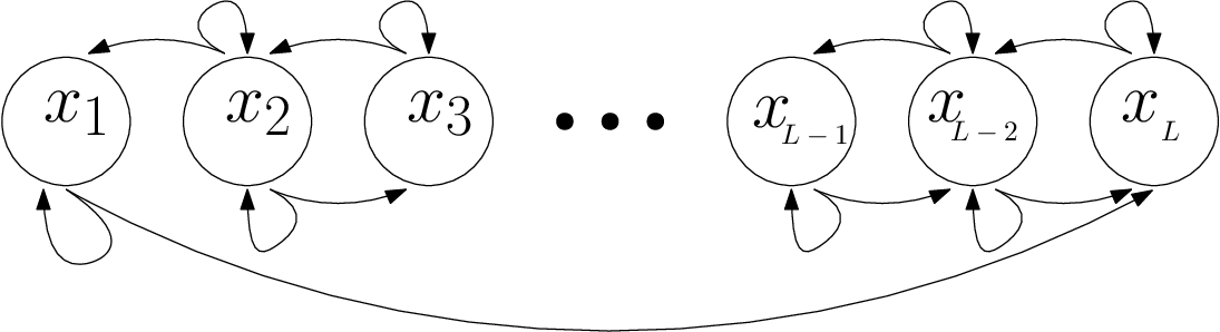
To test our algorithm in this environment, we built $W$ and $F$ taking advantage of the structure of the problem as follows: For $W$, we randomly generate a vector $c$ of length $L$ with entries being 1, 2 or 3. For $i\leq 3$, $W^{\top}_{(x=i,a=\text{left}),j}$=1 if $c_{j}=i$ and 0 otherwise. After that we normalize the three rows, getting three homogeneous non-overlapping distributions. Doing this, we ensure that the realizability assumption is fulfilled for the $\mu_{s}$. We do the same for the “right” action, and we add two more rows with random probability distributions over the whole set of state-action pairs. This makes for a total of 8 rows in $W$.

To build $F$, we also randomly generate a vector $c$ of length $L$ with entries being 1, 2 or 3. For $i\leq 3$, $F_{j,i}=j$ if $c_{j}=j/L$ and 0 otherwise, to guarantee that the relaizability assumption is fulfilled for the $v_{s}$. We also add three random columns with random numbers between 0 and 1, in order to fulfill coherence with high probability. This results in a total of $5$ columns for $F$.

In Figure 4 we show the results obtained with value iteration and the linearly relaxed mirror prox, with $p=0.7$ and different lengths (10 and 100). While for value iteration the number of iterations needed to converge is of the order of the number of states, it is independent of the size of the state space for our algorithm, and rather scales with the number of columns of the matrices $W$ and $F$. This simple example shows that with proper features, our algorithm can actually beat value iteration, which by itself is not able to deal with features.

Our most important contributions concern the relaxed saddle-point problem (2), most notably including our discussion on the necessity and sufficience of the coherence assumption (Assumption 3). As we’ve mentioned earlier, several relaxation schemes similar to ours have been studied in the literature. In fact, relaxing the linear program underlying (1) through the introduction of the feature map $F$ for approximating the value function $v^{*}$ is one of the oldest ideas in approximate dynamic programming, originally introduced by Schweitzer and Seidman 1985. The effects of this approximation were studied by de Farias and Van Roy 2003 in the context of discounted Markov decision processes. A relaxation scheme involving both the feature maps $F$ and $W$ was considered by Lakshminarayanan and Bhatnagar 2015; Lakshminarayanan et al. 2018. Both sets of authors carefully observed that introducing relaxations may make the linear program unbounded, and proposed algorithmic steps and structural assumptions of $F$ and $W$ to fight this issue. The results of these works are incomparable to ours since they focus on controlling the errors in approximating the optimal value function $v^{*}$ rather than controlling the suboptimality of the policies output by the algorithm. Interestingly, the widely popular REPS algorithm of Peters et al. 2010 is also originally derived from the relaxed linear program analyzed by de Farias and Van Roy 2003, even if this connection has not been pointed out by the authors.

The work of Chen et al. 2018 is very close to ours in spirit. Chen et al. 2018 consider a variation of the relaxed saddle-point problem (2) with $W$ being block-diagonal with $F^{\mathsf{\scriptscriptstyle T}}$ in each of its blocks, and claim convergence results for their algorithm to the optimal policy under only a realizability assumption. Unfortunately, their choice of $W$ does not necessarily ensure that the coherence assumption holds, which raises concerns regarding the generality of their guarantees. Indeed, the results of Chen et al. 2018 require an additional assumption that implies that $\frac{\max_{x}d_{\pi}(x)}{\min_{x^{\prime}}d_{\pi}(x^{\prime})}$ remains bounded by a constant for any policy $\pi$, which is extremely difficult to ensure in problems of practical interest. In fact, this ratio is already exponentially large in $|\mathcal{X}|$ in very simple problems like the one we consider in our experiments. Additionally, the analysis of Chen et al. 2018 is based on the potentially erroneous claim that under the realizability assumption, the representation $(u^{*},y^{*})$ of the original optimal solution $(v^{*},\mu^{*})=(Fu^{*},W^{\mathsf{\scriptscriptstyle T}}y^{*})$ always remains an optimal solution to the relaxed saddle-point problem. It is currently unclear if this claim is indeed true, or to what extent their condition regarding the boundedness of stationary distribution can be relaxed.

In any case, we believe that our coherence assumption is more fundamental than the previously considered conditions, and it enables a much more transparent analysis of optimization algorithms addressing the relaxed saddle-point problem (2). Beyond this particular positive result, our work also cleans the slate for further theoretical work on approximate optimization in Markov decision processes. Indeed, the form of our coherence assumption naturally invites the question: can we compute good approximate solutions to the original problem when our assumptions are only satisified approximately? Similar questions are not without precedent in the reinforcement-learning literature. Translated to our notation, classical results concerning the performance of (least-squares) temporal difference learning algorithms imply that the approximation errors are controlled by the projection error of $QFu^{*}+r$ to the column space of $F$ (Tsitsiklis and Van Roy 1997; Bradtke and Barto 1996; Lazaric et al. 2010). When using more general function classes to approximate $v^{*}$, Munos and Szepesvári 2008 show that the approximation errors are controlled by the inherent Bellman error of the function class, which captures an approximation property related to our coherence condition. Whether or not we can generalize our techniques to construct provably efficient algorithms under such milder assumptions remains an exciting open problem that we leave open for future research.

References

- Beck and Teboulle (2003) A. Beck and M. Teboulle. Mirror descent and nonlinear projected subgradient methods for convex optimization. Operations Research Letters, 31(3):167–175, 2003.
- Bellman (1957) R. Bellman. Dynamic Programming. Princeton University Press, Princeton, New Jersey, 1957.
- Bertsekas (2007) D. P. Bertsekas. Dynamic Programming and Optimal Control, volume 2. Athena Scientific, Belmont, MA, 3 edition, 2007.
- Bradtke and Barto (1996) S. J. Bradtke and A. G. Barto. Linear least-squares algorithms for temporal difference learning. Machine Learning, 22:33–57, 1996.
- Bubeck (2015) S. Bubeck. Convex optimization: Algorithms and complexity. Foundations and Trends in Machine Learning, 8(3-4):231–357, 2015.
- Chen et al. (2018) Y. Chen, L. Li, and M. Wang. Scalable bilinear learning using state and action features. In International Conference on Machine Learning, pages 833–842, 2018.
- de Farias and Van Roy (2003) D. P. de Farias and B. Van Roy. The linear programming approach to approximate dynamic programming. Operations Research, 51(6):850–865, 2003.
- de Ghellinck (1960) G. de Ghellinck. Les problèmes de décisions séquentielles. Cahiers du Centre d’Études de Recherche Opérationnelle, 2:161–179, 1960.
- Denardo (1970) E. V. Denardo. On linear programming in a markov decision problem. Management Science, 16(5):281–288, 1970.
- Even-Dar et al. (2009) E. Even-Dar, S. M. Kakade, and Y. Mansour. Online Markov decision processes. Mathematics of Operations Research, 34(3):726–736, 2009.
- Howard (1960) R. A. Howard. Dynamic Programming and Markov Processes. The MIT Press, Cambridge, MA, 1960.
- Konda and Tsitsiklis (1999) V. R. Konda and J. N. Tsitsiklis. Actor-critic algorithms. In S. Solla, T. Leen, and K. Müller, editors, Advances in Neural Information Processing Systems 12, pages 1008–1014, Cambridge, MA, USA, 1999. MIT Press.
- Korpelevich (1976) G. Korpelevich. The extragradient method for finding saddle points and other problems. Matecon, 12:747–756, 1976.
- Lakshminarayanan and Bhatnagar (2015) C. Lakshminarayanan and S. Bhatnagar. A generalized reduced linear program for Markov decision processes. In Proceedings of the Twenty-Ninth AAAI Conference on Artificial Intelligence, AAAI’15, pages 2722–2728. AAAI Press, 2015.
- Lakshminarayanan et al. (2018) C. Lakshminarayanan, S. Bhatnagar, and r. Szepesvári. A linearly relaxed approximate linear program for Markov decision processes. IEEE Transactions on Automatic control, 2018.
- Lazaric et al. (2010) A. Lazaric, M. Ghavamzadeh, and R. Munos. Finite-sample analysis of LSTD. In J. Fürnkranz and T. Joachims, editors, Proceedings of the 27th International Conference on Machine Learning (ICML 2010), pages 615–622. Omnipress, 2010.
- Levin et al. (2017) D. A. Levin, Y. Peres, and E. L. Wilmer. Markov chains and mixing times. 2nd edition. 2017.
- Manne (1960) A. S. Manne. Linear programming and sequential decisions. Management Science, 6(3):259–267, 1960.
- Mnih et al. (2015) V. Mnih, K. Kavukcuoglu, D. Silver, A. A. Rusu, J. Veness, M. G. Bellemare, A. Graves, M. Riedmiller, A. K. Fidjeland, and G. Ostrovski. Human-level control through deep reinforcement learning. Nature, 518(7540):529–533, 2015.
- Munos and Szepesvári (2008) R. Munos and C. Szepesvári. Finite-time bounds for fitted value iteration. Journal of Machine Learning Research, 9(May):815–857, 2008.
- Nemirovski (2004) A. Nemirovski. Prox-method with rate of convergence for variational inequalities with Lipschitz continuous monotone operators and smooth convex-concave saddle point problems. SIAM Journal on Optimization, 15(1):229–251, 2004.
- Nemirovski and Yudin (1983) A. Nemirovski and D. Yudin. Problem Complexity and Method Efficiency in Optimization. Wiley Interscience, 1983.
- Neu et al. (2014) G. Neu, A. György, Cs. Szepesvári, and A. Antos. Online Markov decision processes under bandit feedback. IEEE Transactions on Automatic Control, 59:676–691, 2014.
- Neu et al. (2017) G. Neu, A. Jonsson, and V. Gómez. A unified view of entropy-regularized markov decision processes. arXiv preprint arXiv:1705.07798, 2017.
- Peters et al. (2010) J. Peters, K. Mülling, and Y. Altun. Relative entropy policy search. In Proceedings of the 25th AAAI Conference on Artificial Intelligence (AAAI-10), pages 1607–1612, Menlo Park, CA, USA, 2010. AAAI Press.
- Puterman (1994) M. L. Puterman. Markov Decision Processes: Discrete Stochastic Dynamic Programming. Wiley-Interscience, April 1994.
- Rakhlin and Sridharan (2013a) A. Rakhlin and K. Sridharan. Online learning with predictable sequences. In Conference on Learning Theory, pages 993–1019, 2013a.
- Rakhlin and Sridharan (2013b) A. Rakhlin and K. Sridharan. Optimization, learning, and games with predictable sequences. In Advances in Neural Information Processing Systems, pages 3066–3074, 2013b.
- Schulman et al. (2015) J. Schulman, S. Levine, P. Abbeel, M. Jordan, and P. Moritz. Trust region policy optimization. In Proceedings of the 32nd International Conference on Machine Learning (ICML-15), pages 1889–1897, 2015.
- Schweitzer and Seidman (1985) P. Schweitzer and A. Seidman. Generalized polynomial approximations in Markovian decision processes. J. of Math. Anal. and Appl., 110:568–582, 1985.
- Seneta (2006) E. Seneta. Non-negative matrices and Markov chains. Springer Science & Business Media, 2006.
- Sutton and Barto (2018) R. S. Sutton and A. G. Barto. Reinforcement learning: An introduction. 2nd edition. 2018.
- Sutton et al. (1999) R. S. Sutton, D. A. McAllester, S. P. Singh, and Y. Mansour. Policy gradient methods for reinforcement learning with function approximation. In S. Solla, T. Leen, and K. Müller, editors, Advances in Neural Information Processing Systems 12, pages 1057–1063, Cambridge, MA, USA, 1999. MIT Press.
- Szepesvári (2010) Cs. Szepesvári. Algorithms for Reinforcement Learning. Synthesis Lectures on Artificial Intelligence and Machine Learning. Morgan & Claypool Publishers, 2010.
- Tsitsiklis and Van Roy (1997) J. N. Tsitsiklis and B. Van Roy. An analysis of temporal difference learning with function approximation. IEEE Transactions on Automatic Control, 42:674–690, 1997.
- Wang (2017) M. Wang. Primal-dual learning: Sample complexity and sublinear run time for ergodic Markov decision problems. arXiv preprint arXiv:1710.06100, 2017.
- Zimin and Neu (2013) A. Zimin and G. Neu. Online learning in episodic Markovian decision processes by relative entropy policy search. In C. Burges, L. Bottou, M. Welling, Z. Ghahramani, and K. Weinberger, editors, Advances in Neural Information Processing Systems 26, pages 1583–1591, 2013.
Appendix A Ommitted proofs
A.1 The proof of Lemma 4
The proof will rely on repeatedly using the so-called three-points identity that can easily be shown to hold for all points :
We first use it to show
where we also used the first-order optimality condition for in the second step:
Furthermore, we have
Using this bound together with the three-points identity
we obtain
where the last step follows from the fact that satisfies the first-order optimality condition
Now, using the -strong convexity of and the -Lipschitz continuity of , we obtain
where we also used the elementary inequalities and in the last two steps, respectively. ∎
A.2 The proof of Lemma 8
To enhance readability of the proof, we will omit explicit references to below, and will simply use , and to refer to , and , respectively. Defining for all , we start by noticing that
so all we are left with is bounding the total variation distance between and . To do this, we start by fixing an arbitrary and observing that