Investigating Customization Strategies and Convergence Behaviors of Task-specific ADMM
Abstract
Alternating Direction Method of Multiplier (ADMM) has been a popular algorithmic framework for separable optimization problems with linear constraints. For numerical ADMM fail to exploit the particular structure of the problem at hand nor the input data information, leveraging task-specific modules (e.g., neural networks and other data-driven architectures) to extend ADMM is a significant but challenging task. This work focuses on designing a flexible algorithmic framework to incorporate various task-specific modules (with no additional constraints) to improve the performance of ADMM in real-world applications. Specifically, we propose Guidance from Optimality (GO), a new customization strategy, to embed task-specific modules into ADMM (GO-ADMM). By introducing an optimality-based criterion to guide the propagation, GO-ADMM establishes an updating scheme agnostic to the choice of additional modules. The existing task-specific methods just plug their task-specific modules into the numerical iterations in a straightforward manner. Even with some restrictive constraints on the plug-in modules, they can only obtain some relatively weaker convergence properties for the resulted ADMM iterations. Fortunately, without any restrictions on the embedded modules, we prove the convergence of GO-ADMM regarding objective values and constraint violations, and derive the worst-case convergence rate measured by iteration complexity. Extensive experiments are conducted to verify the theoretical results and demonstrate the efficiency of GO-ADMM.
Index Terms:
Task-specific ADMM, guidance from optimality, convergence behaviors analysis, computer vision applications.I Introduction
Abroad spectrum of real-world applications, ranging from image processing [1, 2] to compressive sensing [3, 4], subspace clustering [5, 6] and machine learning [7, 8], can be (re)formulated as the following separable optimization model with linear constraint:
| (1) |
where and are closed, proper and convex functions, , and . In computer vision and learning scenarios, the fidelity term captures the loss of data fitting, which is further assumed to be continuously differentiable; the regularization/prior term usually is nonsmooth which promotes desired distribution on the solution. To solve Eq. (1), the Alternating Direction Method of Multipliers (ADMM) proposed in [9] becomes a benchmark solver because of its features of easy implementability, competitive numerical performance and wide applicability in various areas.
The ADMM has been receiving attention from a broad spectrum of areas, and various variants have been well studied in the literature. When applying original ADMM to solve Eq. (1) arising from data science applications, how to efficiently solve subproblems plays an important role in the algorithm implementation. To address this issue, plenty of numerical variants have been investigated to tackle subproblems, such as proximal and Linearized ADMM (LADMM) [7, 10, 11], Inexact ADMM (IADMM) [12, 13, 14]. Particularly, in image processing applications, after linearizing the quadratic term, the nonsmooth -subproblem admits a closed form solution. More detailed discussions can be found in survey papers [15, 16]. Unfortunately, even with the proximal or linearizing techniques, for real-world tasks in learning and vision problems, the direct application of these ADMM variants usually leads to performance far from satisfactory. This is because the underlying structure at hand and the input data information have not been well exploited. In fact, these information could help the optimization model find the task-related solution. This motivates us to introduce additional task-specific modules, such as designed filters or trained network architectures, to customize ADMM scheme to address specific applications.
| Types | Methods | Cond. | Fide. | Reg. | Learn. | Opt. | Rate |
| Num. | [17] | and are convex | ✓ | ✓ | ✗ | ✓ | ✓ |
| Task. | [18] | is bounded, is nonexpansive | ✓ | ✗ | ✓ | ✗ | ✗ |
| [19] | is strongly convex, is nonexpansive | ✓ | ✗ | ✓ | ✗ | ✗ | |
| [20] | and are convex, | ✓ | ✓ | ✓ | ✗ | ✗ | |
| Ours | GO-ADMM | and are convex | ✓ | ✓ | ✓ | ✓ | ✓ |
- •
“Cond.” denotes conditions required about , and . “Fide.” represents that the data fidelity term holds. “Reg.” denotes preserving the regularization. “Learn.” implies inserting learning-based information. “Opt.” means iteration sequence converges to the optimal solution of objective. “Rate” represents that convergence rate can be achieved.
Among the ADMMs with embedded task-specific modules, the most prevailing class is introduced in [21], named Plug-and-Play ADMM (PP-ADMM). The PP-ADMM has gained popularity in a broad spectrum of areas, such as super-resolution [22, 18], image denoising [23, 24, 25], inpainting [26] and image reconstruction [19, 27]. The plug-and-play scheme allows one to completely substitute the prior subproblem by manually designed computations within the ADMM scheme. Extremely promising performance has been widely witnessed in image restoration and signal recovery tasks. A variety of task-specific modules has been used for plugging in ADMM framework, ranging from deep-learning-based denoisers [18, 28, 29, 30], Gaussian Mixture Model (GMM) [31, 32] to designed filters [21], etc. However, replacing the prior term with implicit denoising modules usually leads to an unclear definition of the objective function. Consequently, these schemes may fail to guarantee desirable solution qualities. Different from the schemes with implicit priors, Regularization by Denoising (RED) [20] adopts explicit nonconvex regularization with noise evaluation, making the overall objective function clearer and better defined. However, the validity of RED is justified only for denoisers with symmetric Jacobians. Thus, unfortunately, many state-of-the-art methods, such as BM3D [33], RF [34], CSF [35], CNN [36] cannot be covered; this issue has been discussed in [37]. Recently, deep learning-based methods have become state-of-the-art. Douglas-Rachford Network (Dr-Net) [38] and learning deep CNN denoiser prior [36] apply ConvNets modeling data fidelity and/or image prior proximal operators. Like these learning-based schemes, aiming at obtaining data-specific iteration schemes, ADMMNet [8, 39] introduced hyperparameters into the classical numerical solvers and then performed discriminative learning on collected training data. The existing learning-based methods perform better on vision tasks than many state-of-the-art methodologies. Due to the severe inconstancy of parameters during iterations, rigorous analysis of the resulted trajectories is also missing, which leads to the lack of strict theoretical investigations. Methods based on optimal conditions [40, 41, 4] reduced the gap between deep networks and optimization models by introducing error control condition. For example, in [40], the implicit ADMM scheme converges to a fixed point while without knowing whether it is an optimal solution to the objectives. For a clear impression, we summarize the essential comparison aspects in Tab. I.
I-A Our Contributions
Numerical ADMM cannot exploit the particular structure of the problem at hand nor the input data information and thus may fail in learning and visual problems. The existing task-specific schemes plug their task-specific modules into the numerical iterations in a straightforward manner. Even with some restrictive constraints on the plug-in modules, they can only obtain some relatively weaker convergence properties for the resulted ADMM iterations. Thus, leveraging task-specific modules (e.g., neural networks and other data-driven architectures) to extend ADMM is an important but challenging problem. To partially address issues in these existing task-specific methods, this work constructed a completely new algorithmic framework to design task-specific ADMM. In this paper, we propose the Guidance from Optimality (GO)-ADMM, which incorporates a mechanism to embed task-specific modules into the fidelity subproblem. The new paradigm aggregates both data fidelity and ad-hoc modules, and the prior information is reserved during iteration processes. Theoretical convergence in previous works (e.g., [18, 42, 19]) often requires certain architecture constraints on the embedded modules (e.g., boundedness, nonexpansive or Lipschitz conditions). Unfortunately, verification of these assumptions is too ambitious, especially when the task-specific modules are explicitly complex deep network architectures. One notable feature of the proposed GO-ADMM relies on the fact that a first-order-optimality-based guiding policy is involved during each iteration. Thanks to this feature, the convergence of GO-ADMM is independent of any architecture constraint. This new perspective enables us to automatically identify reliable modules to build our task-specific iterations. We further rigorously prove the convergence of GO-ADMM towards a solution. Besides, we analyze the convergence rate in terms of iteration complexity. To our best knowledge, GO-ADMM seems to be the first theoretically convergent task-specific ADMM, whose convergence, surprisingly as good as those well-designed numerical ADMMs, requires no additional assumptions on embedded modules. The main contributions of this work are summarized as:
- •
A striking feature of GO-ADMM, which differs from previous approaches is that a new mechanism is incorporated to embed modules into the fidelity subproblem. Thanks to this design, we aggregate data fidelity and ad-hoc modules, with prior information kept in reserve for our task-specific iterations.
- •
Different from existing schemes that usually require certain architecture constraints on the additional modules, GO-ADMM adopts an optimality-based guiding policy to automatically identify reliable modules, resulting in a self-controllable propagation scheme.
- •
We strictly prove the global convergence towards a solution with quality and estimate the exact convergence rate. Our theoretical results indeed inherit analytic properties of well-designed numerical ADMM, and thus are more convincing than those existing heuristic task-specific methods.
- •
Extensive experiments verify our theories. In particular, we can observe performance even better than some state-of-the-art deep learning methods. Furthermore, our GO strategy could be extended to other first-order schemes, achieving rigorous convergence results.
II Review on Existing ADMMs
Specifically, by introducing the augmented Lagrangian function of Eq. (1) with multiplier and penalty parameter
the standard ADMM scheme reads as
| (2) | ||||
| (3) | ||||
| (4) |
which can be understood as iteratively performing the alternating minimization for the primal variables (, ) and gradient ascent for the dual variable . Typically, is smooth and is nonsmooth.
Task-specific Schemes: The implementations of a variant of task-specific ADMM algorithms do not need a specified regularization/prior term . Instead, they adopt an off-the-shelf image denoising module to replace -subproblem. A wide range of task-specific modules have been plugged into the ADMM framework, such as CSF [35], BM3D [33, 18], GMM [32, 31], Non-Local Means (NLM) [42, 43], deep learning based denoiser [36, 44] and denoising autoencoders [45], and etc. According to the characteristics of optimization models, we roughly separate them into two parts: explicit task-specific schemes and implicit task-specific schemes.
Implicit task-specific schemes build on the use of an implicit prior, which regularizes general inverse problems. For example, the plug-and-play ADMM (firstly introduced in [21]) replaces the -subproblem by an implicit off-the-shelf algorithm. Furthermore, the alternating minimization for the primal variables (, ) can be regarded as two independent numerical modules, i.e., one for implementing a simplified reconstruction operator and the other for performing a denoising operator (such as [38]). The modified scheme by incorporating a continuation form has been introduced in [18, 46, 42, 29, 19]. In particular, the iteration step is updated by using an off-the-shelf nonexpansive denoising operator. However, the objective function is not clearly defined if arbitrary denoising engines are used. Consequently, this may lead to undesirable convergence results.
Explicit schemes explicitly leverage the natural image distribution as prior. In this category, RED [20, 37], Block Coordinate RED (BC-RED) [28], and deep RED [47] have gained much significance in recent years. Explicit schemes rely on a general structured smoothness penalty term to regularize the desired inverse problem with a constructed denoising module. Nevertheless, these explicit regularization forms lack supervision for the iteration steps. Moreover, the existing convergent results are less convincing.
Learning data-fidelity term has drawn much attention recently [48, 38]. For example, in [48], a discriminative framework is used to learn the data term (i.e., -subproblem) in a cascaded manner. In [38], Dr-Net framework is developed to replace the proximal operator in both the data fidelity term and the prior term with two different networks that firmly satisfy the non-expansive condition. A drawback of these learning data-fidelity frameworks is the lacking of theoretical guarantees.
In summary, different from existing numerical variants of ADMM in which usually show weak performance in real-world applications, the proposed GO-ADMM allows any off-the-shelf modules of imaging systems to be inserted into ADMM scheme and achieves state-of-the-art results. Different from the task-specific ADMMs which usually require certain conditions of these specific modules and are prone to introduce unclear structures that may change the objective function, we rigorously prove the convergence of the established task-specific schemes according to objective function values and constraint violation with a flexible module and easy-to-calculate error control policy. Moreover, we analysis the convergence rate in terms of the iteration complexity. It is worth noting that our investigations not only reduce the gap between the practical implementations of ADMM and the strict convergence analyze for task-specific approaches but also provide a computationally feasible and theoretically guaranteed manner to address convex optimization in real-world application scenarios.
III The Proposed GO-ADMM
As aforementioned, most existing task-specific ADMM schemes perform the task-specific computational modules, instead of the non-differentiable subproblem (i.e., Eq. (3)). Consequently, they fail to preserve the well-designed priors in the original optimization formulation. Notably, strict convergence properties (e.g., the global convergence to the original model and the exact convergence rate estimation) cannot be adequately guaranteed. In this section, we propose a new task-specific algorithmic framework, namely, the GO-ADMM, to address the above two fundamental issues.
Specifically, GO-ADMM aims to incorporate task information into the subproblem w.r.t. . The differentiable objective of the optimization model in Eq. (1) characterizes the fidelity/loss information of the task. In most learning and vision applications, the variables in this term are always measured after some given linear mappings (e.g., the degradation operation, mask matrix, transformation, and/or additional errors). Therefore, hereafter we further specify , where denotes a task-related linear mapping, and refers to the measurement which is continuously differentiable and strongly convex. Many commonly used fidelity/loss functions (e.g., quadratic, exponential, and logistic losses) can be formulated as such specific .
III-A Non-Euclidean Proximal Regularization
Instead of generating an iterative trajectory in Euclidean space as in standard ADMM, we first introduce a general proximal regularization for Eq. (5). Specifically, we define a proximal term at the -th iteration as , where defines a task-specific general metric (including Euclidean and non-Euclidean metrics) and will be specified for particular applications in Sec. V. In this way, the -update reads as
| (5) |
Particularly, is a flexible scheme that can incorporate particular task information (e.g., mask, filter) or hyper-parameter into the optimization process. If is a real number, means Euclidean metric, while if we set as a mask or filter, implies non-Euclidean metric. In addition, the involvement of also improves the computational performance in the differentiable subproblem (i.e., Eq. (5)), which will be clarified in the following subsection.
III-B Differentiable Updating with Modules Ensemble
Now we design a new updating rule to further perform task-specific computations for the differentiable subproblem in Eq. (5). Specifically, the -subproblem can be reformulated as the following linear system
| (6) |
where . By defining the following operation on
and assuming that is invertible11 1 We can easily obtain this invertible property by introducing a invertible metric matrix ., it is easy to see that solving Eq. (5) is equivalent to finding an approximate solution of the system .
In standard ADMM scheme, one may directly adopt numerical techniques to solve this equation.22 2 This solution can be derived with a closed-form solution or iterative methods. For quadratic cases, the approximate solution can be obtained either by an iterative method such as Preconditioned Conjugate Gradient (PCG) [49] or direct method such as Cholesky factorization [50]. For nonlinear cases, we can employ gradient descent or Newton-type methods to solve this system. In contrast, we introduce an auxiliary variable to integrate the original updating trajectory and the (designed and/or trained) task-specific computations as follows
| (7) |
where denotes a given task-specific module and is an adaptive averaging parameter which reflects the influence of task-specific modules. Our algorithmic framework does not request any specific assumptions for the computational module . Indeed, we incorporate the guidance policy to automatically adjust the influence factor . That is, improper can be eliminated. In a consequence, the formal updating of reads as
| (8) |
III-C The Guidance of Optimality (GO) Policy
To navigate the above task-specific iterations towards desired optimal solutions, we introduce a new policy, named Guidance of Optimality (GO), to identify the properly nested module and control the iteration trajectory. Specifically, we define an error term to measure the inexactness of our performed task-specific computation as follows
| (9) |
Upon together Eqs. (6), (8) and (9), we have
Therefore, can be quantitatively regarded as the difference between the task-specific solution of -subproblem generated by GO-ADMM and the exact solution obtained by standard ADMM in Eq. (2), in the sense of the partial gradient residual from the augmented Lagrangian function. Inspired by this observation, we introduce the following relaxed condition as our guidance policy:
| (10) |
where is a constant. In this way, if the task-specific computation in Eq. (8) satisfies the inequality in Eq. (10), we actually obtain a proper updating for the differentiable subproblem. Rather, we should reduce the influence of the nested module, until it does not work for our iterations. So in the worst case, GO-ADMM will temporarily reduce to a standard ADMM at some iterations if improper computational modules are utilized. Overall, our GO-ADMM algorithmic framework is summarized in Alg. 1.
Remark 1.
We argue that our error condition (i.e., Eq. (10)) can always be satisfied in Alg. 1, for parameter is dramatically decreasing while iterations. Thus, in the worst case, Eq. (10) will be satisfied when . Actually, equation reduces to as . Then, iteration of -subproblem is a pure numerical scheme and one may directly adopt numerical techniques to solve this equation. We summarize the numerical algebra solver as and explain this numerical scheme as follows. For quadratic cases of function , the approximate system is linearized and its solution can be obtained either by an iterative method such as Preconditioned Conjugate Gradient (PCG) or direct method such as Cholesky factorization. For example, we consider the instance , , , , . For this case, we have . Thus, -subproblem becomes and the solution can be derived by closed-form solution, i.e., . With the defined error term , the above closed-form solution implies
Based on the above formulation, we have . Also, we can apply PCG or Cholesky factorization to obtain the approximate solution until satisfying . For nonlinear cases, we can employ gradient descent or Newton-type methods to find satisfying Eq. (10).
Remark 2.
As for , our algorithmic framework actually does not rely directly on any specific assumptions for these computational modules and the guidance policy in Section III can automatically reduce the influence up to reject these improper .
IV Theoretical Investigations
In this section, we investigate the convergence behaviors of task-specific iterations within the proposed GO-ADMM paradigm. Rather than enforcing restrictive constraints on these nested modules, here we consider the following mild assumptions on the function defined in Sec. III.
Assumption 1.
For , satisfies that
| (11) |
and its gradient is Lipschitz continuous such that
| (12) |
where and are two positive constants.
The following definitions are used in the sequel. Let and denote . Then define the operator and the matrix as follows:
| (13) |
where denotes the diagonal array. Note that is not necessarily positive definite because the matrix in Eq. (1) is not assumed to be full column rank.
We first reformulate Eq. (1) into a Variational Inequality (VI). This reformulation helps to analyze convergent properties via VI approach. As initiated in [51], the Lagrangian function of Eq. (1) is defined as
where is Lagrangian multiplier. Let be a saddle point of the Lagrangian function. Then for any , satisfies
| (14) |
With specified , then . Note that these first-order optimal conditions (i.e. Eq. (14)) can be written in a compact form
| (15) |
Thus, the VI can be designed as finding , , that satisfies the above VI inequality (15). Actually, throughout the work, we consider the case of practical interest that the KKT solution set of Eq. (15) is nonempty. Now we are ready to present our theoretical results. Specifically, to prove the convergence of the sequence generated by GO-ADMM, it is crucial to analyze how the residual evolves according to the iterations. For this reason, we first provide the following proposition.
Proposition 1.
Let be the sequence defined in Eq. (9), and are the sequences generated by GO-ADMM. If constant satisfies
| (16) |
with , then we have the following inequality
| (17) |
where .
Now we prove the convergence of the sequence generated by GO-ADMM. To simplify the notation, we denote
| (18) |
In fact, this notation is not required to be practically calculated when implementing GO-ADMM. Then in the following proposition, we analyze the difference between defined in Eq. (18) and the solution point formulated by Eq. (15).
Proposition 2.
The difference between the inequality in Eq. (19) and the variational inequality reformulation in Eq. (15) reflects the difference between the point and a solution point . For the right-hand side of Eq. (19), the second term (i.e., three quadratic terms) is easy to be manipulated over different indicators by algebraic operations, but it is not clear about how to control the crossing term (i.e., ) towards the eventual goal, i.e., illustrate the convergence of the sequence . We thus explore this term particularly and derive that the sum of these crossing terms over iterations can be bounded by some quadratic terms as well. This result is summarized in the following proposition.
Proposition 3.
Let be the sequence generated by GO-ADMM. For all , and , it holds that
| (20) |
Now we establish the convergence results of GO-ADMM in the following theorem.
Theorem 1.
Let be the sequence generated by the GO-ADMM and denote as the solution set of the variational inequality in Eq. (15). Then, we have the following assertions:
- 1.
, and .
- 2.
, and for any given .
It is easy to verify that is a solution of Eq. (15) if and only if and . Hence, it is reasonable to measure the accuracy of the iterate by and .
Corollary 1.
The upper bounds of and is in order of . That is, our proposed GO-ADMM actually obtains worst-case convergence rate in a non-ergodic sense.
Remark 3.
Instant of making assumptions on directly, we suppose that is invertible. This invertible property can be easily obtained by introducing an invertible metric matrix . Second, we must clarify that in this work we provide general theoretical results. The convergence regarding is actually , without making any assumption on . Trivially, if is full column rank, we can obtain immediately. It is worth mentioning that, in image processing tasks (the object is usually formulated as ), we often reformulate these problems to general forms (i.e, , s.t., ) by introducing where is an auxiliary variable. In this case, is denoted as a negative identity matrix (i.e., ) which must be full column rank.
 |
 |
 |
 |
 |
| (a) | (b) | (c) | (d) | (e) |
|
 |
 |
 |
 |
V Applications
As a nontrivial byproduct, we first demonstrate how to apply GO-ADMM to image restoration problems in real-world low-level vision applications, such as image denoising, inpainting, and compressed sensing MRI tasks. Then, we illustrate the implementation of GO-ADMM to tackle more difficult rain streaks removal problems that we estimate rain streaks and background simultaneously.
Image Restoration: Individually, we consider the following Total Variation (TV) minimization model that is popularly performed in various low-level computer vision tasks, especially in image processing problems. Then we define the model as
where , denote the latent and observed image respectively, and is a linear operator. represents the gradient of in horizontal and vertical directions. By introducing variable , the above equation can be transformed into the following form
| (21) |
Next, applying GO-ADMM to Eq. (21), we have that
where . Now, we are ready to design inner iterative strategy to update . First, the task-specific module is designed as a denoiser operator. Then the candidate variable can be rewritten as . If satisfies the error control condition (10), we set , else decrease the weight by to obtain the candidate . Actually, if , we estimated by solving the following linear equation
with PCG method as stated in Subsection III-B satisfying which is defined as in (16). Then, variables of , and are updated following Alg. 1.
Rain Streaks Removal: For rain streaks removal application, we reformulate this problem with unknown background layer and rain streaks layer by the setting function and , where and denotes the rainy image. In this case, we set as block unit matrix, i.e., . By introducing two auxiliary variables and , we reformulate Eq. (1) as follows
By introducing the dual multipliers and the penalty parameter , generalized updates form of variables are summarized as follows
Indeed, for and -subproblems, we set and as the denoiser and rain streaks removal operators respectively with different input (i.e., and ). We then follow the form in image restoration applications to update and .
 |
 |
 |
 |
 |
VI Numerical Results
This section first conducts experiments to verify our theoretical results. Then we compare the performance of the proposed algorithm scheme with other state-of-the-art methods in real-world problems, such as image denoising, inpainting, compressed sensing MRI, and rain streaks removal. All experiments are performed on a PC with Intel Core i7 CPU at 3.2 GHz, 32 GB RAM and a NVIDIA GeForce GTX 1070 GPU.
VI-A Numerical Validation
To verify the convergence properties of the proposed approach, this subsection is organized as follows: We first apply our algorithm on image denoising that aims to restore the latent grayscale or color image from the corrupted observation which relies on the linear model to analyze the iterative behaviors and the error conditions with different settings. In this application, we set as a unit matrix. Then, to make a further analysis, we illustrate the convergence behaviors of the proposed scheme on a general form. Here, we conduct experiments on image deconvolution, , that aims to recover the unknown latent image from the missing pixels of the observation with the mask matrix and the noise . Detailed analyses are provided in the following.
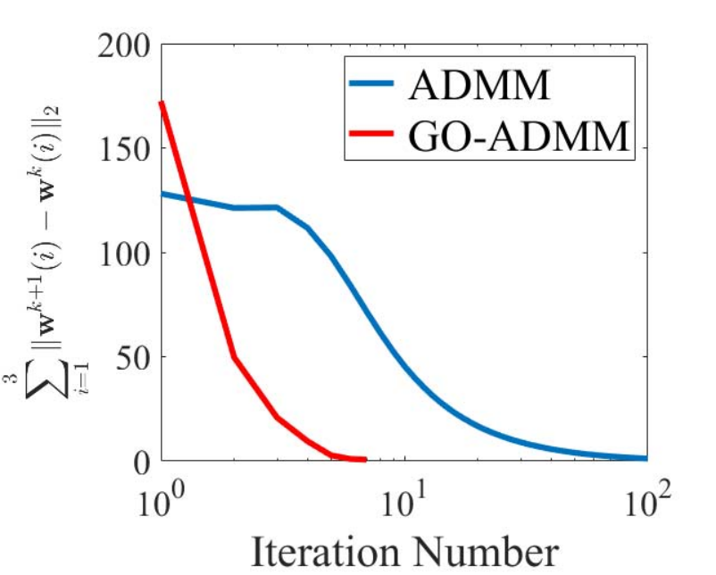
We first compare the proposed method with standard ADMM in image denoising application with noise level and the corresponding metrics are plotted in Fig. 1. To calculate the performance, we plotted the PSNR curves in Fig. 1(a). Observed that the proposed GO-ADMM performed the best with fewer iteration steps when compared with standard ADMM. Indeed, the task-specific module is used to calculate a task-related optimal solution that plays a critical part in real-world applications. To further compare the convergence of GO-ADMM with other numerical ones, we plotted the iteration errors (i.e., where is defined in (18)) in Fig. 1(b). Moreover, we provide a detailed analysis of the convergence by showing the errors about , and (i.e., plotted in Fig. 1(c), (d), and (e) respectively). Note that, in image denoising applications, is the gradient operator and denotes the identity matrix. Moreover, Fig. 1(b)-(e) verified the convergence theories provided in Theorem 1.
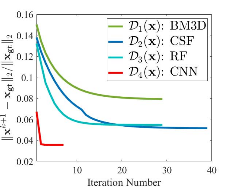
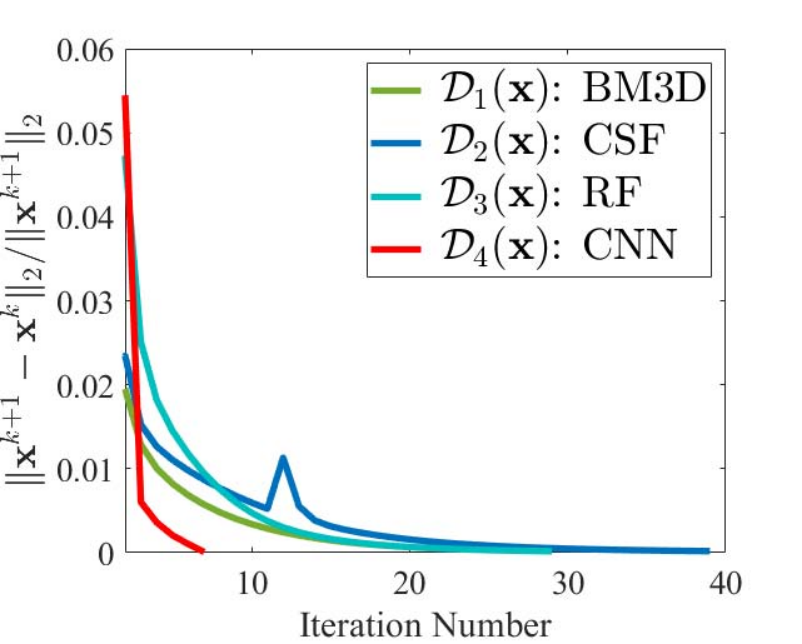
To illustrate the flexibility of the task-specific module in GO-ADMM, we then consider the performance of GO-ADMM with four different strategies for settings, such as filtering (BM3D [33], RF [34]), discriminant learning (CSF) [35], and the convolution neural networks (CNNs) [36], in image denoising task under noise level. The corresponding convergence behaviors are plotted in the first four subfigures of Fig. 2 with reconstruction errors, relative errors (), and iterative errors of the dual variable (i.e., ). These subfigures illustrate that different settings have distinct effects on experimental performance and convergent behaviors. Observed that GO-ADMM with CNNs strategy performed the best than the others (i.e., with BM3D, CSF, RF settings). Consequently, we set the task-specific module as a set of CNNs in the following work. Additionally, it is crucial to show the guidance behaviors (i.e., the error control condition and as described in Eq. (9)) under CNNs setting when conduct the experiment. Then, the corresponding curves are plotted in Fig. 2 (e) in which denotes the lower bound of . As for the estimation of , we have that , where is the minimum characteristic value of and with . Thus, we have . In this experiment, parameters and are set as and , respectively. With , the relationship between and is satisfied. Clearly, experimental results imply that iterations with CNNs module met the error control condition stated in Eq. (10) (i.e., ). Further, convergent behaviors in Fig. 2 shows that GO-ADMM has no limit on the task-specific module .
As for , we actually train a series of CNNs on images with different noise levels or rain streaks in image derain task as our “bank” of modules. As for CNNs, we just adopt the standard residual architecture, consisting of nineteen layers, i.e., seven dilated convolutions with filter size, six ReLu operations (plugged between each two convolution layers) and five batch normalizations (plugged between convolution and ReLU, except the first convolution layer). In the training phase of image denoising, deblurring and inpainting, we randomly sample 800 natural images from the ImageNet database [52] and add Gaussian noise with different noise levels. In rain streaks removal application, we select Rain100L [53] and Rain1400 [54] datasets to train the CNNs. We use ADAM with a weight decay of 0.0001 to optimize MSE loss to train our network. The learning rate is initially set as 0.001 and decayed by multiplying 0.1 at the 30th, 60th and 80th epochs. As for , in image denoising, inpainting and MRI applications, it is selected as a parameter. In rain streaks removal task, is designed as rain streaks mask measured by CNN networks.
 |
 |
To evaluate the effectiveness of regularization/prior knowledge and inserted data information, we conduct an ablation experiment on image deconvolution application with a noise level, and the corresponding results are shown in Fig. 3. In this experiment, represents a blurry kernel. Observed that, Fig. 3 attributes the effectiveness of prior term and inserted data information.
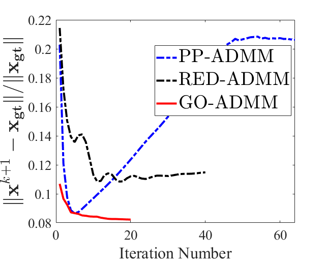
We further conduct an experiment on image deblurring task to compare the proposed method with implicit and explicit plug-in form (i.e., PP-ADMM and RED-ADMM). As shown in Fig. 4, PP-ADMM and RED-ADMM curves are oscillating. This is mainly because the introduced denoiser does not satisfy the strict smoothness and symmetrical structure required in RED-ADMM, and also does not meet the non-expansive requirement in PP-ADMM. Fortunately, GO-ADMM has no demand for the proposed task-specific module directly. In other words, the introduced guidance policy prevents the iteration sequence from tending to unwanted solutions.
VI-B State-of-the-Art Comparisons
Image Denoising. Image denoising aims to restore the latent grayscale or color image from the corrupted observation that relies on the linear model . Here we compared our GO-ADMM with several state-of-the-art image restoration approaches, including plug-in methods (PP-ADMM [18], RED-ADMM [20]) and learning-based methods (DnCNN [55], CBDNet [56]). We conducted experiments on the challenging real-world noisy image provided in [57] and the corresponding results are shown in Fig. 5. Observed that our method removes more noise and restores a clearer image than the compared approaches.
 |
 |
 |
 |
 |
| PP-ADMM | RED-ADMM | DnCNN | CBDNet | Ours |
 |
 |
 |
 |
 |
 |
| 19.86 / 0.32 | 28.77 / 0..82 | 26.69 / 0.82 | 28.67 / 0.80 | 28.89 / 0.82 | 29.54 / 0.84 |
| ISDSB | FoE | WNNM | IRCNN | LBS | Ours |
| Mask | FoE | ISDSB | WNNM | IRCNN | LBS | Ours |
| 34.01 | 31.32 | 31.75 | 34.92 | 34.54 | 34.96 | |
| 0.90 | 0.91 | 0.94 | 0.95 | 0.95 | 0.98 | |
| 30.81 | 28.23 | 28.71 | 31.45 | 31.27 | 31.56 | |
| 0.81 | 0.83 | 0.89 | 0.91 | 0.90 | 0.91 | |
| 27.64 | 24.92 | 25.63 | 26.44 | 27.71 | 27.89 | |
| 0.65 | 0.70 | 0.78 | 0.79 | 0.80 | 0.81 | |
| Text | 37.05 | 34.91 | 34.89 | 37.26 | 36.88 | 37.47 |
| 0.95 | 0.96 | 0.97 | 0.97 | 0.94 | 0.98 |
 |
 |
 |
 |
 |
 |
| Input | PANO (29.75) | FDLCP (29.99) | BM3D-MRI (28.97) | TGDOF (32.06) | Ours (32.30) |
Image Inpainting. In image inpainting task, the matrix denotes mask, and represents the missing pixels image. Then, we conducted experiments on image inpainting to recover missing pixels from observation. Here we compared our GO-ADMM with FOE [58], ISDSB [59], WNNM [60], IRCNN [36], and LBS [44] on this task. We generated random masks of different levels (i.e., , , and ) and missing pixels on the CBSD68 dataset [55]. Further, we use 12 different text masks to evaluate the developed approach. The comparison results are listed in Tab. II with averaged quantitative results (PSNR and SSIM scores). Regardless of the proportion of masks, our GO-ADMM can achieve better performance when compared with the other methods. Furthermore, the visual performance of missing pixels are shown in Fig. 6. It can be seen that the proposed method outperformed all the compared methods on both visualization and metrics (PSNR and SSIM).
| Methods | Cartesian | Radial | Gaussian | |||
| PSNR | RLNE | PSNR | RLNE | PSNR | RLNE | |
| ZeroFilling | 23.95 | 0.2338 | 27.66 | 0.1524 | 26.80 | 0.1683 |
| TV | 26.30 | 0.1790 | 31.11 | 0.1032 | 32.45 | 0.0885 |
| SIDWT | 25.77 | 0.1896 | 31.44 | 0.0994 | 32.49 | 0.0880 |
| PANO | 29.73 | 0.1206 | 33.49 | 0.0786 | 36.98 | 0.0527 |
| FDLCP | 29.65 | 0.1218 | 34.31 | 0.0713 | 38.26 | 0.0452 |
| ADMMNet | 27.72 | 0.1520 | 33.31 | 0.0802 | 36.56 | 0.0550 |
| BM3D-MRI | 28.86 | 0.1330 | 34.59 | 0.0692 | 39.16 | 0.0410 |
| TGDOF | 31.30 | 0.1007 | 35.47 | 0.0625 | 39.75 | 0.0382 |
| Ours | 31.33 | 0.1003 | 35.51 | 0.0622 | 39.93 | 0.0374 |
 |
 |
 |
 |
 |
 |
| DDN | UGSM | JORDER | DID-MDN | PReNet | Ours |
Compressed Sensing MRI. In compressed sensing Magnetic Resonance Imaging (MRI) task, we define as under-sampling matrix and Fourier transformation [8], i.e., . We randomly choose 25 -weighted MRI data from 50 different subjects in IXI datasets 33 3 http://brain-development.org/ixi-dataset/ as the testing data for our comparison. Then we adopt three types of sampling masks, i.e., Cartesian pattern [61], Radial pattern [8], and Gaussian mask [62] on selected -weighted dataset. We compare our GO-ADMM with ZeroFilling [63], TV [64], SIDWT [65], PANO [66], FDLCP [67], ADMMNet [8], BM3D-MRI [68], and TGDOF [27], and the comparison results are shown in Tab. III. Observed that, our paradigm shows great superiority in reconstruction accuracy and has a better ability to accommodate sampling patterns. We then provide the visual comparisons in Fig. 7 for three methods with relatively high PSNR and RLNE scores (i.e., PANO, FDLCP, and TGDOF). Consistently, our GO-ADMM achieves the best performance in terms of both the restoration of detail and the PSNR scores.
| Methods | Rain100L | Rain1400 | Rain100H | |||
| PSNR | SSIM | PSNR | SSIM | PSNR | SSIM | |
| DN | 27.27 | 0.8746 | 25.51 | 0.8885 | 13.72 | 0.4417 |
| DDN | 29.73 | 0.9177 | 29.90 | 0.8999 | 17.93 | 0.5655 |
| UGSM | 28.59 | 0.8772 | 26.38 | 0.8261 | 14.90 | 0.4674 |
| JORDER | 36.61 | 0.9722 | 27.50 | 0.8515 | 23.45 | 0.7490 |
| DID-MDN | 25.45 | 0.8550 | 27.94 | 0.8696 | 17.28 | 0.6035 |
| PReNet | 37.63 | 0.9792 | 32.32 | 0.9320 | 29.46 | 0.8990 |
| Ours | 37.64 | 0.9792 | 32.57 | 0.9319 | 29.50 | 0.8990 |
| Ours (w) | 37.76 | 0.9798 | 32.64 | 0.9320 | 29.51 | 0.8991 |
Rain Streaks Removal. To evaluate the performance of our method, we use both synthetic test data and real-world images to compare our approach with state-of-the-art approaches (including DerainNet (DN) [69], Deep Detailed Network (DDN) [54], JORDER [70], UGSM [71], DID-MDN [72], and PReNet [73]) removing rain from single images. For measuring the performance quantitatively, we employ PSNR, SSIM as the metrics. All the comparisons shown in this paper are conducted under the same hardware configuration.
Tab. IV shows the results of different methods on Rain100L, Rain100H [53], and Rain1400 [54] datasets. As observed, our method considerably outperforms others in terms of both PSNR and SSIM. Fig. 8 compares the visual performance of GO-ADMM to the first five scores methods listed in Tab. IV on real-world challenging rainy image. Observed that DDN tends to retain excessive rain streaks while GMM tends to keep rain streaks for images with over-smooth background details. Qualitatively, the proposed GO-ADMM achieves the best visual results in terms of effectively removing the rain streaks while preserving the scene details. We further evaluate the performance with designed . Here, are selected as rain streaks mask measured by CNN networks [36]. We also listed the GO-ADMM results with designed (i.e., GO-ADMM (w)) in Tab. IV.
VII Conclusions
In this paper, we proposed a collaborative learning scheme with the task-specific flexible module for specific optimization problems to solve vision and learning tasks. We provided strict theoretical analysis for the proposed GO-ADMM by introducing an error based criterion condition to measure the inexactness of the inner iterations. Further, the experimental results verified that GO-ADMM can even obtain better performance against most other state-of-the-art approaches.
Appendix A Proofs
We first provide some preparations. Since we just adopt standard computation strategy in Eqs. (3)-(4) to update - and -subproblems, the first-order optimality condition for sequence generated by our GO-ADMM can be summarized as
| (22) |
For convenience, we denote , and .
A-A Proof of the Proposition 1
Proof.
Recall that the - and -subproblems are assumed to be solved exactly in the GO-ADMM. We thus know that and thus
| (23) |
Hence, it is easily derived that
| (24) |
With the definition of in Eq. (9), we have
where and . Therefore, it follows that
with . This relationship will be often used in the coming analysis. This complete the proof. ∎
A-B Proof of the Proposition 2
Proof.
First we rewrite as
Then for all , the following holds
where . Combining it with the optimality (22), the above inequality yields that
Moreover, notice the elementary equation
| (25) |
We denote the right hand of Eq. (25) as . Thus, for all , we have
where and has the similar form with and . The proof is complete. ∎
A-C Proof of the Proposition 3
A-D Proof of the Theorem 1
Proof.
First, we define and recall the definition of in (13). We have
| (27) |
Then, using the results (19) and Propositions 2 and 3, respectively, we obtain
| (28) |
For any given , we have , . Setting in (28), together with the above property, for any , we have
Recall that the parameter controlling the accuracy in (10) is restricted by the condition (16). Hence, it follows from the definition of that and obviously there exists a such that As we conclude that Furthermore, for any , there exists such that for all , we have For all , it follows from (26) that
which implies that Moreover, note that can be obtained by the fact . The first assertion is proved.
Now we prove the second assertion. For the first part: , it follows immediately from the facts and . Note that the optimality conditions of the -subproblem at the (+)-th iteration and a solution point can be respectively written as
Accordingly, taking and respectively in the above inequalities, we have
| (29) |
The same technique can also be applied to the -subproblem and a solution point . Additionally, using the convexity of , we have
| (30) |
Then, summarizing (29) and (30), we obtain
| (31) |
Since , as well as and
both the left- and right-hand sides of (31) converge to zero. As a result, we have which is the second assertion of this theorem. The proof is complete. ∎
A-E Proof of the Corollary 1
Proof.
The proof of this Corollary can be conducted following the same road-maps developed in [14]. Indeed, from inequality (28), it is easy to show the upper bound of is in order of . With the help of inequality (26), one can also obtain the upper bound of with the same order. The details of the proof are similar to [14] and we do not repeat it here. ∎
Acknowledgment
This work is partially supported by the National Key R&D Program of China (2020YFB1313503), the National Natural Science Foundation of China (Nos. 61922019, 61672125, 61733002, 61432003, 61632019, 11971220), Shenzhen Science and Technology Program (No. RCYX20200714114700072), the Stable Support Plan Program of Shenzhen Natural Science Fund (No. 20200925152128002), Guangdong Basic and Applied Basic Research Foundation 2019A1515011152, and the Fundamental Research Funds for the Central Universities.
References
- [1] R. H. Chan, J. Yang, and X. Yuan, “Alternating direction method for image inpainting in wavelet domains,” SIAM Journal on Imaging Sciences, vol. 4, no. 3, pp. 807–826, 2011.
- [2] M. Ng, F. Wang, and X.-M. Yuan, “Fast minimization methods for solving constrained total-variation superresolution image reconstruction,” Multidimensional Systems and Signal Processing, vol. 22, no. 1-3, pp. 259–286, 2011.
- [3] J. Yang and Y. Zhang, “Alternating direction algorithms for -problems in compressive sensing,” SIAM journal on scientific computing, vol. 33, no. 1, pp. 250–278, 2011.
- [4] R. Liu, S. Cheng, Y. He, X. Fan, Z. Lin, and Z. Luo, “On the convergence of learning-based iterative methods for nonconvex inverse problems,” IEEE Trans. Pattern Anal. Mach. Intell., 2019.
- [5] G. Liu, Z. Lin, S. Yan, J. Sun, Y. Yu, and Y. Ma, “Robust recovery of subspace structures by low-rank representation,” IEEE Trans. Pattern Anal. Mach. Intell., vol. 35, no. 1, pp. 171–184, 2013.
- [6] E. Elhamifar and R. Vidal, “Sparse subspace clustering: Algorithm, theory, and applications,” IEEE Trans. Pattern Anal. Mach. Intell., vol. 35, no. 11, pp. 2765–2781, 2013.
- [7] R. Liu, Z. Lin, and Z. Su, “Linearized alternating direction method with parallel splitting and adaptive penalty for separable convex programs in machine learning,” in Asian Conference on Machine Learning, 2013, pp. 116–132.
- [8] J. Sun, H. Li, Z. Xu et al., “Deep admm-net for compressive sensing mri,” in Proc. Advances in Neural Inf. Process. Systems., 2016, pp. 10–18.
- [9] R. Glowinski and A. Marroco, “Sur l’approximation, par éléments finis d’ordre un, et la résolution, par pénalisation-dualité d’une classe de problèmes de dirichlet non linéaires,” ESAIM: Mathematical Modelling and Numerical Analysis-Modélisation Mathématique et Analyse Numérique, vol. 9, no. R2, pp. 41–76, 1975.
- [10] J. Yang and X. Yuan, “Linearized augmented lagrangian and alternating direction methods for nuclear norm minimization,” Mathematics of computation, vol. 82, no. 281, pp. 301–329, 2013.
- [11] X. Xie, J. Wu, Z. Zhong, G. Liu, and Z. Lin, “Differentiable linearized admm,” in Proc. Int. Conf. Mach. Learn., 2019.
- [12] X.-M. Yuan, “The improvement with relative errors of he et al.’s inexact alternating direction method for monotone variational inequalities,” Mathematical and computer modelling, vol. 42, no. 11-12, pp. 1225–1236, 2005.
- [13] J. Eckstein and W. Yao, “Relative-error approximate versions of douglas–rachford splitting and special cases of the admm,” Mathematical Programming, vol. 170, no. 2, pp. 417–444, 2018.
- [14] H. Yue, Q. Yang, X. Wang, and X. Yuan, “Implementing the alternating direction method of multipliers for big datasets: A case study of least absolute shrinkage and selection operator,” SIAM Journal on Scientific Computing, vol. 40, no. 5, pp. A3121–A3156, 2018.
- [15] S. Boyd, N. Parikh, E. Chu, B. Peleato, J. Eckstein et al., “Distributed optimization and statistical learning via the alternating direction method of multipliers,” Foundations and Trends® in Machine learning, vol. 3, no. 1, pp. 1–122, 2011.
- [16] R. Glowinski, “On alternating direction methods of multipliers: a historical perspective,” in Modeling, simulation and optimization for science and technology. Springer, 2014, pp. 59–82.
- [17] B. He and X. Yuan, “On non-ergodic convergence rate of douglas–rachford alternating direction method of multipliers,” Numerische Mathematik, vol. 130, no. 3, pp. 567–577, 2015.
- [18] S. H. Chan, X. Wang, and O. A. Elgendy, “Plug-and-play admm for image restoration: Fixed-point convergence and applications,” Trans. Comput. Imaging,, vol. 3, no. 1, pp. 84–98, 2017.
- [19] E. K. Ryu, J. Liu, S. Wang, X. Chen, Z. Wang, and W. Yin, “Plug-and-play methods provably converge with properly trained denoisers,” Proc. Int. Conf. Mach. Learn., 2019.
- [20] Y. Romano, M. Elad, and P. Milanfar, “The little engine that could: Regularization by denoising (red),” SIAM Journal on Imaging Sciences, vol. 10, no. 4, pp. 1804–1844, 2017.
- [21] S. V. Venkatakrishnan, C. A. Bouman, and B. Wohlberg, “Plug-and-play priors for model based reconstruction,” in Global Conference on Signal and Information Processing. IEEE, 2013, pp. 945–948.
- [22] K. Zhang, W. Zuo, and L. Zhang, “Deep plug-and-play super-resolution for arbitrary blur kernels,” in Proceedings of the IEEE Conference on Computer Vision and Pattern Recognition, 2019, pp. 1671–1681.
- [23] W. Dong, P. Wang, W. Yin, G. Shi, F. Wu, and X. Lu, “Denoising prior driven deep neural network for image restoration,” IEEE Trans. Pattern. Anal. Mach. Intell., vol. 41, no. 10, pp. 2305–2318, 2018.
- [24] G. T. Buzzard, S. H. Chan, S. Sreehari, and C. A. Bouman, “Plug-and-play unplugged: Optimization-free reconstruction using consensus equilibrium,” SIAM Journal on Imaging Sciences, vol. 11, no. 3, pp. 2001–2020, 2018.
- [25] A. Rond, R. Giryes, and M. Elad, “Poisson inverse problems by the plug-and-play scheme,” Journal of Visual Communication and Image Representation, vol. 41, pp. 96–108, 2016.
- [26] T. Tirer and R. Giryes, “Image restoration by iterative denoising and backward projections,” IEEE Trans.Image Process., vol. 28, no. 3, pp. 1220–1234, 2018.
- [27] R. Liu, Y. Zhang, S. Cheng, Z. Luo, and X. Fan, “Converged deep framework assembling principled modules for cs-mri,” IEEE Trans. Medical Imaging, 2020.
- [28] Y. Sun, J. Liu, and U. Kamilov, “Block coordinate regularization by denoising,” in Proc. Advances in Neural Inf. Process. Systems., 2019, pp. 380–390.
- [29] T. Meinhardt, M. Moller, C. Hazirbas, and D. Cremers, “Learning proximal operators: Using denoising networks for regularizing inverse imaging problems,” in Proc. IEEE Conf. Int. Conf. Comput. Vis., 2017, pp. 1781–1790.
- [30] S. Liu, E. Reehorst, P. Schniter, and R. Ahmad, “Free-breathing cardiovascular mri using a plug-and-play method with learned denoiser,” ISBI, 2020.
- [31] Y. Li, R. T. Tan, X. Guo, J. Lu, and M. S. Brown, “Rain streak removal using layer priors,” in Proc. IEEE Conf. Comput.Vis.Parttern Recognit., 2016.
- [32] A. M. Teodoro, J. M. Bioucas-Dias, and M. A. Figueiredo, “A convergent image fusion algorithm using scene-adapted gaussian-mixture-based denoising,” IEEE Trans.Image Process., vol. 28, no. 1, pp. 451–463, 2019.
- [33] K. Dabov, A. Foi, V. Katkovnik, and K. Egiazarian, “Image denoising by sparse 3-d transform-domain collaborative filtering,” IEEE Trans. Image Process., vol. 16, no. 8, pp. 2080–2095, 2007.
- [34] E. S. Gastal and M. M. Oliveira, “Domain transform for edge-aware image and video processing,” in ACM Transactions on Graphics, vol. 30, no. 4. ACM, 2011, p. 69.
- [35] U. Schmidt and S. Roth, “Shrinkage fields for effective image restoration,” in Proc. IEEE Conf. Comput. Vis. Pattern Recognit., 2014, pp. 2774–2781.
- [36] K. Zhang, W. Zuo, S. Gu, and L. Zhang, “Learning deep cnn denoiser prior for image restoration,” in Proc. IEEE Conf. Comput. Vis. Pattern Recognit., 2017, pp. 3929–3938.
- [37] E. T. Reehorst and P. Schniter, “Regularization by denoising: Clarifications and new interpretations,” Trans. Comput. Imaging,, vol. 5, no. 1, pp. 52–67, 2018.
- [38] R. Aljadaany, D. K. Pal, and M. Savvides, “Douglas-rachford networks: Learning both the image prior and data fidelity terms for blind image deconvolution,” in Proc. IEEE Conf. Comput.Vis.Parttern Recognit., 2019, pp. 10 235–10 244.
- [39] Y. Yang, J. Sun, H. Li, and Z. Xu, “Admm-net: A deep learning approach for compressive sensing mri,” arXiv preprint arXiv:1705.06869, 2017.
- [40] R. Liu, X. Fan, S. Cheng, X. Wang, and Z. Luo, “Proximal alternating direction network: A globally converged deep unrolling framework,” in Proc. AAAI Conf. Artif. Intell, 2018.
- [41] Y. Wang, R. Liu, X. Song, and Z. Su, “Linearized alternating direction method with penalization for nonconvex and nonsmooth optimization,” in Proc. AAAI Conf. Artif. Intell, 2016.
- [42] S. H. Chan, “Performance analysis of plug-and-play admm: A graph signal processing perspective,” IEEE Trans. Comput.Imaging, vol. 5, no. 2, pp. 274–286, 2019.
- [43] S. Sreehari, S. V. Venkatakrishnan, B. Wohlberg, G. T. Buzzard, L. F. Drummy, J. P. Simmons, and C. A. Bouman, “Plug-and-play priors for bright field electron tomography and sparse interpolation,” IEEE Trans. Comput.Imaging, vol. 2, no. 4, pp. 408–423, 2016.
- [44] R. Liu, S. Cheng, Y. He, X. Fan, and Z. Luo, “Toward designing convergent deep operator splitting methods for task-specific nonconvex optimization,” arXiv preprint arXiv:1804.10798, 2018.
- [45] S. A. Bigdeli, M. Zwicker, P. Favaro, and M. Jin, “Deep mean-shift priors for image restoration,” in Proc. Advances in Neural Inf. Process. Systems., 2017, pp. 763–772.
- [46] Y. Sun, B. Wohlberg, and U. S. Kamilov, “An online plug-and-play algorithm for regularized image reconstruction,” Trans. Comput. Imaging,, 2019.
- [47] G. Mataev, P. Milanfar, and M. Elad, “Deepred: Deep image prior powered by red,” in Proc. IEEE Int. Conf. Comput. Vis. Workshops, 2019, pp. 0–0.
- [48] J. Dong, J. Pan, D. Sun, Z. Su, and M.-H. Yang, “Learning data terms for non-blind deblurring,” in Proc. European Conf. Comput. Vis., 2018, pp. 748–763.
- [49] S. C. Eisenstat, “Efficient implementation of a class of preconditioned conjugate gradient methods,” SIAM Journal on Scientific and Statistical Computing, vol. 2, no. 1, pp. 1–4, 1981.
- [50] Y. Chen, T. A. Davis, W. W. Hager, and S. Rajamanickam, “Algorithm 887: Cholmod, supernodal sparse cholesky factorization and update/downdate,” ACM Trans. on Mathematical Software, vol. 35, no. 3, pp. 1–14, 2008.
- [51] B. He and X. Yuan, “On the o(1/n) convergence rate of the douglas–rachford alternating direction method,” SIAM Journal on Numerical Analysis, vol. 50, no. 2, pp. 700–709, 2012.
- [52] O. Russakovsky, J. Deng, H. Su, J. Krause, S. Satheesh, S. Ma, Z. Huang, A. Karpathy, A. Khosla, M. Bernstein et al., “Imagenet large scale visual recognition challenge,” IJCV, vol. 115, no. 3, pp. 211–252, 2015.
- [53] D. Martin, C. Fowlkes, D. Tal, and J. Malik, “A database of human segmented natural images and its application to evaluating segmentation algorithms and measuring ecological statistics,” in Proc. IEEE Conf. Int. Conf. Comput. Vis., 2001, pp. 416–423.
- [54] X. Fu, J. Huang, D. Zeng, Y. Huang, X. Ding, and J. Paisley, “Removing rain from single images via a deep detail network,” in Proc. IEEE Conf. Comput.Vis.Parttern Recognit., 2017.
- [55] K. Zhang, W. Zuo, Y. Chen, D. Meng, and L. Zhang, “Beyond a gaussian denoiser: Residual learning of deep cnn for image denoising,” IEEE Trans. Image Process., vol. 26, no. 7, pp. 3142–3155, 2017.
- [56] S. Guo, Z. Yan, K. Zhang, W. Zuo, and L. Zhang, “Toward convolutional blind denoising of real photographs,” in Proc. IEEE Conf. Comput.Vis.Parttern Recognit., 2019, pp. 1712–1722.
- [57] M. Lebrun, M. Colom, and J.-M. Morel, “The noise clinic: a blind image denoising algorithm,” Image Processing On Line, vol. 5, pp. 1–54, 2015.
- [58] S. Roth and M. J. Black, “Fields of experts,” International Journal of Computer Vision, vol. 82, no. 2, p. 205, 2009.
- [59] L. He and Y. Wang, “Iterative support detection-based split bregman method for wavelet frame-based image inpainting,” IEEE Trans. Image Process., vol. 23, no. 12, pp. 5470–5485, 2014.
- [60] S. Z. Li, Markov random field modeling in image analysis. Springer Science & Business Media, 2009.
- [61] X. Qu, D. Guo, B. Ning, Y. Hou, Y. Lin, S. Cai, and Z. Chen, “Undersampled mri reconstruction with patch-based directional wavelets,” Magnetic resonance imaging, vol. 30, no. 7, pp. 964–977, 2012.
- [62] G. Yang, S. Yu, H. Dong, G. Slabaugh, P. L. Dragotti, X. Ye, F. Liu, S. Arridge, J. Keegan, Y. Guo et al., “Dagan: deep de-aliasing generative adversarial networks for fast compressed sensing mri reconstruction,” IEEE transactions on medical imaging, vol. 37, no. 6, pp. 1310–1321, 2018.
- [63] M. A. Bernstein, S. B. Fain, and S. J. Riederer, “Effect of windowing and zero-filled reconstruction of mri data on spatial resolution and acquisition strategy,” Journal of Magnetic Resonance Imaging: An Official Journal of the International Society for Magnetic Resonance in Medicine, vol. 14, no. 3, pp. 270–280, 2001.
- [64] M. Lustig, D. Donoho, and J. M. Pauly, “Sparse mri: The application of compressed sensing for rapid mr imaging,” Magnetic Resonance in Medicine: An Official Journal of the International Society for Magnetic Resonance in Medicine, vol. 58, no. 6, pp. 1182–1195, 2007.
- [65] R. G. Baraniuk, “Compressive sensing,” IEEE signal processing magazine, vol. 24, no. 4, 2007.
- [66] X. Qu, Y. Hou, F. Lam, D. Guo, J. Zhong, and Z. Chen, “Magnetic resonance image reconstruction from undersampled measurements using a patch-based nonlocal operator,” Medical image analysis, vol. 18, no. 6, pp. 843–856, 2014.
- [67] Z. Zhan, J.-F. Cai, D. Guo, Y. Liu, Z. Chen, and X. Qu, “Fast multiclass dictionaries learning with geometrical directions in mri reconstruction,” IEEE Transactions on Biomedical Engineering, vol. 63, no. 9, pp. 1850–1861, 2016.
- [68] E. M. Eksioglu, “Decoupled algorithm for mri reconstruction using nonlocal block matching model: Bm3d-mri,” Journal of Mathematical Imaging and Vision, vol. 56, no. 3, pp. 430–440, 2016.
- [69] X. Fu, J. Huang, X. Ding, Y. Liao, and J. Paisley, “Clearing the skies: A deep network architecture for single-image rain removal,” IEEE Trans. Image Process., vol. 26, no. 6, 2017.
- [70] W. Yang, R. T. Tan, J. Feng, J. Liu, Z. Guo, and S. Yan, “Deep joint rain detection and removal from a single image,” in Proc. IEEE Conf. Comput. Vis. Pattern Recognit., 2017.
- [71] T.-X. Jiang, T.-Z. Huang, X.-L. Zhao, L.-J. Deng, and Y. Wang, “Fastderain: A novel video rain streak removal method using directional gradient priors,” IEEE Trans. Image Process., 2018.
- [72] H. Zhang and V. M. Patel, “Density-aware single image de-raining using a multi-stream dense network,” in Proc. IEEE Conf. Comput. Vis. Pattern Recognit., 2018.
- [73] D. Ren, W. Zuo, Q. Hu, P. Zhu, and D. Meng, “Progressive image deraining networks: a better and simpler baseline,” in Proc. IEEE Conf. Comput.Vis.Parttern Recognit., 2019, pp. 3937–3946.
![[Uncaptioned image]](1909.10819v2/RishengLiu.png) |
Risheng Liu received the B.S. and Ph.D. degrees both in mathematics from the Dalian University of Technology in 2007 and 2012, respectively. He was a visiting scholar in the Robotic Institute of Carnegie Mellon University from 2010 to 2012. He served as Hong Kong Scholar Research Fellow at the Hong Kong Polytechnic University from 2016 to 2017. He is currently a professor with DUT-RU International School of Information Science & Engineering, Dalian University of Technology. He was awarded the “Outstanding Youth Science Foundation” of the National Natural Science Foundation of China. His research interests include machine learning, optimization, computer vision and multimedia. He was a co-recipient of the IEEE ICME Best Student Paper Award in both 2014 and 2015. His two papers were also selected as Finalist of the Best Paper Award in ICME 2017. He is a member of the IEEE and ACM. |
![[Uncaptioned image]](1909.10819v2/PanMu.png) |
Pan Mu received the B.S. degree in Applied Mathematics from Henan University, China, in 2014, the M.S. degree in Operational Research and Cybernetics from Dalian University of Technology, China, in 2017. She is currently pursuing the PhD degree in Computational Mathematics at Dalian University of Technology, China. Her research interests include computer vision, machine learning and optimization. |
![[Uncaptioned image]](1909.10819v2/JinZhang.png) |
Jin Zhang received the B.A. degree in Journalism from the Dalian University of Technology in 2007. He pursued a degree in mathematics and received the M.S. degree in Operational Research and Cybernetics from the Dalian University of Technology, China, in 2010, and the PhD degree in Applied Mathematics from University of Victoria, Canada, in 2015. After working in Hong Kong Baptist University for 3 years, he joined Southern University of Science and Technology as a tenure-track assistant professor in the Department of Mathematics. His broad research area is comprised of optimization, variational analysis and their applications in economics, engineering and data science. |