Precision Model-Independent Bounds from Global Analysis of Form Factors
Abstract
We present a model-independent global analysis of hadronic form factors for the semileptonic decays that exploits lattice-QCD data, dispersion relations, and heavy-quark symmetries. The analysis yields predictions for the relevant form factors, within quantifiable bounds. These form factors are used to compute the semileptonic ratios and various decay-product polarizations. In particular, we find and , predictions that can be compared to results of upcoming LHCb measurements. In developing this treatment, we obtain leading-order NRQCD results for the nonzero-recoil relations between the form factors.
I Introduction
While the Higgs interaction is the only source of lepton universality violations within the Standard Model (SM), the observation of neutrino masses implies that at least one form of beyond-SM modification exists, specifically in the lepton sector. The factorization of QCD dynamics from electroweak interactions in the SM allows amplitudes for semileptonic decays to be expressed as the familiar product of hadron () and lepton () tensors at leading order:
| (1) |
Heavy-hadron semileptonic decay rates (both full and differential) producing distinct lepton flavors differ only due to factors of lepton mass that arise from kinematic and chirality-flip factors. Such dependences can be removed in a variety of ways Colangelo and De Fazio 2018; Ivanov et al. 2016; Tran et al. 2018; Bhattacharya et al. 2016; Bhattacharya et al. 2017; Jaiswal et al. 2017; Bhattacharya et al. 2019; Cohen et al. 2018a; Bečirević et al. 2019. Measurements from BaBar, Belle, and LHCb of the ratios Lees et al. 2012; Lees et al. 2013; Huschle et al. 2015; Abdesselam et al. 2019a; Sato et al. 2016; Aaij et al. 2015; Hirose et al. 2017; Aaij et al. 2018a; Aaij et al. 2018b; Hirose et al. 2018 of the heavy-light meson decays , with to , exhibit a combined 3.1 discrepancy from the HFLAV-suggested SM values Amhis et al. 2017, which average Refs. Bigi and Gambino 2016; Bernlochner et al. 2017; Bigi et al. 2017; Jaiswal et al. 2017. Recently, the LHCb collaboration has measured Aaij et al. 2018c, which is within 1.3 Cohen et al. 2018b of the SM prediction. These results, including lattice-determined and theoretically computed values of , are compiled in Table 1.
| 0.340(27)(13) Lees et al. 2012; Lees et al. 2013; Huschle et al. 2015; Abdesselam et al. 2019a | 0.300(8) Aoki et al. 2019; Na et al. 2015; Bailey et al. 2015 | 0.299(3) Amhis et al. 2017 | |
| 0.295(11)(8) Lees et al. 2012; Lees et al. 2013; Huschle et al. 2015; Sato et al. 2016; Aaij et al. 2015; Hirose et al. 2017; Aaij et al. 2018a; Aaij et al. 2018b; Hirose et al. 2018; Abdesselam et al. 2019a | – | 0.258(5) Amhis et al. 2017 | |
| – | 0.2987(46) McLean et al. 2019a | – | |
| – | 0.3328(74)(70) Detmold et al. 2015 | 0.324(4)Bernlochner et al. 2018 | |
| 0.71(17)(18) Aaij et al. 2018c | [0.20,0.39] Cohen et al. 2018b | – | |
| – | 0.30(4) Berns and Lamm 2018; Murphy and Soni 2018 | – |
In the future, it would be useful to consider other semileptonic decays. Run III of LHCb may open the opportunity to measure Cerri et al. 2018. A determination of would be exciting. However, is substantially harder to measure than for a few reasons, foremost of which is the absence of a clean decay process with a substantial branching fraction (analogous to ) for reconstructing the ; this leads to large backgrounds. Additionally, the transition from excited charmonium states to is poorly understood, which further complicates the extraction of signals Hamilton and Jawahery.
In order to fully leverage all of these experimental results, it is necessary to have rigorous predictions from the SM for all of these ratios. Even setting aside the very interesting issue of lepton universality, determining hadronic form factors is important in its own right, as each such function represents a wealth of information about nonperturbative QCD. Form factors are not completely unconstrained, however. They must satisfy well-known model-independent constraints that follow from bedrock principles of quantum field theory, specifically unitarity and the complex analyticity of their Green’s functions as functions of momentum variables at all values, except when a resonance, particle-creation threshold, or other special kinematic configuration is realized. In the case of semileptonic decays, the form factors can be parametrized as a product of known functions representing resonant poles and other nonanalytic structures in the corresponding Green’s function, times a Taylor series in a conformal variable that tracks the momentum transfer; the Taylor coefficients are constrained in magnitude by unitarity. This is the BGL parametrization Boyd et al. 1995a; Boyd et al. 1997 (see Ref. Grinstein and Lebed 2015 for a brief review of its historical antecedents).
The constraint of unitarity in model-independent approaches such as the BGL parametrization has historically been underutilized, because fits to experiment typically consider only a single exclusive process (e.g., ). However, each exclusive channel appearing in the two-point Green’s function for currents positively contributes to the unitarity bound, and therefore a simultaneous fit including multiple processes provides stronger constraints on each of the individual processes Boyd et al. 1997; Bigi et al. 2017; Jaiswal et al. 2017.
The purpose of this work is to perform a global analysis within the BGL parametrization of lattice-QCD data for seven exclusive hadronic processes: , , , and . We obtain the corresponding transition form factors. These form factors are computed directly from the SM and obtained within quantifiable bounds. Thus, they can be used to make reliable predictions from the SM that can directly confront experiment. We use them to compute three types of observables: the semileptonic decay ratios , the polarization , and the vector-meson longitudinal polarization fraction .
The analysis presented here is essentially model independent. We do not use ad hoc model assumptions about the physical mechanisms dominating the form factor, beyond accepting the SM to identify allowed functional forms of the form factors. Rather, we use as input ab initio Monte Carlo calculations of QCD from the lattice as our principal input. Such data is quite limited: not all of the relevant form factors have been computed, and those that have are computed at a limited number of momentum-transfer values. The BGL parametrization using the unitarity bound allows us to extend our knowledge of the form factors to other momentum transfers, and to do so in such a way that the errors can be quantified. We can gain information about form factors that have not been directly computed on the lattice from those that have by exploiting emergent symmetries of QCD that become valid as the quark masses become large.
There are, of course, errors associated with truncating the series in BGL parametrization and truncating the expansion in the inverse heavy-quark mass. Fortunately, one has a priori estimates of their size, which allows for reliable SM predictions without invoking additional model dependence. However, some judgment is required in estimating their sizes quantitatively. We have therefore made very conservative estimates in order to ensure that our predicted bounds are reliable enough so that the experimental measurements provide meaningful tests of the SM.
The lattice data that provides the input for the analysis has both statistical and systematic errors. The statistical errors can be easily incorporated into our bounds. In some cases the major systematic errors have been well-explored and estimated reliably, and can also be incorporated in a straightforward way. However, in some cases the only available lattice calculations do not provide estimates for some of the major systematic errors. In these cases, we add a systematic error in by hand, and do so in a very conservative manner, by assuming larger-than-realistic errors.
Thus, while the analysis is model independent, it does involve some ad hoc judgment in the assignment of systematic errors. As this was done quite conservatively, the principal effect is to make the error bounds for our final results larger than they otherwise would be. These effects can, of course, be mitigated by the constant improvement in the treatment of errors in lattice simulations.
We begin in Sec. II with a discussion of the weak-interaction structure of the SM responsible for semileptonic decays and the form factors under investigation. In Sec. III we explain how heavy-quark symmetries can be used to obtain relations between the form factors of heavy-light systems and heavy-heavy meson systems. The lattice results used in this work are discussed in Sec. IV. Section V presents the dispersive-analysis framework utilized to constrain the form factors as functions of momentum transfer. The results of our analysis are presented in Sec. VI, and we conclude in Sec. VII.
II Structure of
Since the first-principles calculation of the leptonic tensor in Eq. (1) is straightforward in the SM, the computation of semileptonic decay rates reduces to parametrizing exclusive components of the hadronic tensor in terms of transition form factors. The tensor structure is expressed in terms of the hadron momenta, for (with mass ) and for (with mass ), and additionally the polarization of the if it is a vector meson, or heavy-quark spinors if are baryons. The only functional dependence of the form factors arises through the squared momentum transfer to the leptons, . The various cases of phenomenological interest are now outlined.
II.1
If both are pseudoscalar mesons, then only two independent Lorentz structures, and hence two independent form factors, are possible:
| (2) | |||||||
Indeed, the parity invariance of strong interactions precludes the current from providing a nonzero contribution to Eq. (2). In this work, we exchange for the combination
| (3) |
With this definition, one sees that , a constraint upon two otherwise independent form factors that we will impose when fitting the functions. This normalization of differs by a mass-dependent prefactor from that used in lattice-QCD calculations Colquhoun et al. 2016; Lytle; Aoki et al. 2019; Na et al. 2015; Bailey et al. 2015; McLean et al. 2019a:
| (4) |
The differential decay rate for this semileptonic decay process is
| (5) |
where, in terms of the spatial momentum of in the rest frame,
| (6) |
in which we have, in turn, introduced two important kinematic values, .
II.2
Transition form factors of a pseudoscalar meson to a vector meson have been parametrized in a variety of ways in the literature. Here, we begin with a set Wirbel et al. 1985 of vector [] and axial-vector [] form factors frequently used in lattice-QCD and model calculations:
| (7) |
where . Only four of these five form factors are independent: demanding that only couples to timelike virtual polarizations () requires
| (8) |
Requiring the cancellation of terms in Eq. (II.2) as imposes the additional constraint .
A different decomposition, in which the virtual and vector meson are described by their helicity states, turns out to be more useful for the dispersive analysis. Here, one exchanges the form factors for the set . They are related by
| (9) |
, are proportional to the conventionally defined Richman and Burchat 1995 helicity amplitudes , respectively, while the other two helicity amplitudes are linear combinations of and form factors, , where is defined in Eq. (6).
At , the middle two expressions of Eqs. (9) reduce to an additional constraint, . In this basis, the previously noted constraint becomes . The differential decay rate for the semileptonic decay in this basis reads
| (10) |
II.3
In the case of heavy-baryon transitions, the states of the spin- baryons are represented by spinors . Here, there are two form factors for both the vector and axial-vector currents:
where the kinematical variables relevant to the heavy-quark limit (see Sec. III) are the baryon 4-velocities, and . The differential decay rate is then
| (12) |
where the form factors in helicity basis read
| (13) |
As in the meson case, these form factors satisfy exact constraints at special kinematic points. Specifically, , , and . This basis differs from that used in the lattice-QCD calculations of Ref. Detmold et al. 2015 only by mass-dependent prefactors:
| (14) |
III Heavy-Quark Symmetries
The physics of heavy-light hadrons ( or is simplified by the emergence of additional symmetries in the limit . Operators distinguishing between heavy quarks of different spin orientation and flavor are suppressed by , and produce a vanishingly small effect upon physical amplitudes in the heavy-quark limit. All transition form factors between two hadrons with a single heavy quark and the same light-quark content are proportional to a single, universal Isgur-Wise function, Isgur and Wise 1989; Isgur and Wise 1990 for mesons or for baryons Mannel et al. 1991. They are naturally expressed , which is the dot product of the initial and final heavy-light hadron 4-velocities, and , respectively, and fully contains the information about :
| (15) |
The zero-recoil point, where the final hadron is created at rest in the rest frame of the initial hadron , satisfies , corresponding to . From the middle expressions of Eq. (15), one notes that is the Lorentz factor of in the rest frame. The maximum value of in a given semileptonic process occurs when the momentum transfer through the virtual to the lepton pair—the total energy-squared of the leptons in their rest frame—assumes its smallest possible value, .
Heavy-quark symmetry encodes a physical picture in which a heavy-light hadron is described by a nearly static color-fundamental source with spin-independent interactions (the heavy quark ), to which the matter associated with light degrees of freedom (light-quarks and gluons) is bound. In weak decays with , the zero-recoil (Isgur-Wise) point corresponds to a situation in which spontaneously transforms to at rest, but the decay otherwise leaves the light degrees of freedom undisturbed. The overlap between the initial and final light-quark wave functions is complete, so that or at the zero-recoil (Isgur-Wise) point. Thus, in the heavy quark limit one obtains an absolute normalization for the form factors; in the meson case Isgur and Wise 1989; Isgur and Wise 1990; Boyd et al. 1997, all the form factors are proportional to :
| (16) |
while in the baryon case Mannel et al. 1991, all the form factors are proportional to :
| (17) |
where . All of these results are corrected by effects of .
Due to the lack of lattice data for , we use the relations of Eq. (III) for and to obtain for each of the processes from the existing lattice data. To establish a first approximation for an allowed region, we parametrize by
| (18) |
In our analysis we have included an additional systematic error of 20% to account for violations of Isgur-Wise scaling. We sample three synthetic points from for each form factor. For , the synthetic points are restricted to the same range for as the lattice data. For , where lattice results have been computed in the full range, we restrict the synthetic points to the near-zero-recoil range of .
In decays of the types , the spectator quark can no longer be considered light (and indeed is the same species as the final heavy quark). These cases are more complicated; the heavy-quark limit differs from the heavy-light case in two important ways Jenkins et al. 1993. First, the heavy-quark kinetic-energy operators for and quarks, while both scaling as , differ for the two flavors (thus breaking the heavy-quark flavor symmetry), but still provide leading-order corrections to the dynamics of the state due to the presence of the heavy spectator : e.g., the Bohr radii of and are significantly different. Second, the spectator receives a momentum transfer due to the transition of the same order as the momentum imparted to the . Thus, the heavy-flavor symmetry due to the replacement of with does not leave the spectator degrees of freedom invariant, meaning that one cannot obtain a normalization of the form factors at the zero-recoil point based purely upon symmetry.
Even though the heavy-flavor symmetry obtained from replacing with is lost, the and quarks retain separate heavy-quark spin symmetries, as does the heavy spectator . In addition, since the valence quarks are heavy these systems are better described using nonrelativistic dynamics than are heavy-light systems. Indeed, for , a sufficiently modest value that suggests information obtained near the zero-recoil point remains phenomenologically useful. The six meson form factors of Eqs. (2) and (9) are related by the spin symmetries to a single, universal function that Ref. Jenkins et al. 1993 calls , and Ref. Kiselev et al. 2000 calls . However, as emphasized in Ref. Jenkins et al. 1993, the form factors only approach near the zero-recoil point, and its normalization there is not fixed by symmetry to assume a special value, like .
A central feature of Ref. Jenkins et al. 1993 is the use of the trace formalism of Ref. Falk et al. 1990 to compute the relative normalization between the six meson form factors (i.e., to obtain the correct multiple of for each tensor structure) near the zero-recoil point. To be specific, “near” in this sense means kinematic configurations in which the spatial momentum transfer to the spectator is no larger than its mass . This calculation was generalized in Refs. Kiselev et al. 2000; Kiselev using NRQCD to consider a small-recoil limit () in which the four-velocities of and are nevertheless unequal (i.e., the spectator receives a momentum transfer at leading order in NRQCD). These relations were used in Refs. Cohen et al. 2018b; Berns and Lamm 2018; Murphy and Soni 2018 to constrain the form factors at zero recoil.
In this work, we extend the relations of Refs. Kiselev et al. 2000; Kiselev by deriving the leading-order NRQCD relations between the form factors and at non-zero recoil. While these relations are expected to receive large corrections away from , we use them to construct ratios of derivatives of form factors at . To proceed, we start with the trace formalism of Ref. Falk et al. 1990:
| (19) |
where are the velocities of the spectator quark, decaying quark, and final-state quark respectively. These velocities are related in the heavy-quark limit to those of the mesons by , , and , where
| (20) |
with and . One can then use the trace formalism to obtain the -dependent generalizations of the constants defined in Refs. Kiselev et al. 2000; Kiselev. Starting with the tensor definitions
| (21) | |||||
where
| (22) |
we construct the Isgur-Wise-like relations for the heavy-heavy systems:
| (23) |
These relations reproduce the standard Isgur-Wise results Isgur and Wise 1989; Isgur and Wise 1990; Boyd et al. 1997 of Eq. (III) in the limit , and they reduce to the relations of Refs. Kiselev et al. 2000; Kiselev when . Terms that break these relations should be , and, in our analysis we conservatively allow for up to 50% violations. We use these relations in our analysis to fix both the relative normalization between form factors and their slopes at zero recoil. These results are obtained by constructing ratios from Eqs. (III) after solving for and .
IV Lattice QCD Results
This work we uses the existing lattice-QCD results for form factors as input to our global analysis. These results have been produced by a number of different groups, and the determinations of the various form factors have been performed at varying numbers of momentum-transfer values and with varying treatments of uncertainties. In this section we summarize the lattice results used in our analysis.
The best current results are those for form factors. The form factors and have been computed by two groups Na et al. 2015; Bailey et al. 2015, including a complete treatment of all sources of error. We use the results of Bailey et al. 2015 alone in the final results, having found that the larger uncertainties of Na et al. 2015 mean that they provide no significant additional constraint.
For the case of , a single group has produced results for and at non-zero recoil with a complete error treatment McLean et al. 2019a. The baryonic process has been computed in Ref. Detmold et al. 2015 on only one lattice volume, but their results include a 1.5% systematic uncertainty for finite-volume effects, and given a quantified error estimate, we can include this lattice data in our analysis.
The heavy-heavy process has also only been computed by one group Colquhoun et al. 2016; *ALE, with an incomplete treatment of errors. It was computed on a single lattice volume, so finite-volume effects are potentially worrying. To account for possible large finite-volume effects, in the analysis we included an additional 20% systematic error.
In the process , the two form factors and have been reported at non-zero recoil by one group on one lattice volume Colquhoun et al. 2016; *ALE. For these form factors, we also include an additional 20% systematic error. For the other two form factors, and , no results have been presented.
For the final two processes and , only the zero-recoil value of [which is exactly related to at zero recoil, see above Eq. (II.2)] has been computed. In the case of , has been computed by two groups Bailey et al. 2014; Harrison et al. 2018, and here we take the FLAG value Aoki et al. 2019. For , we include the recent result of Ref. McLean et al. 2019b. In addition to the lack of non-zero recoil data, no results for and at any points are available.
The presentation of these results in the literature is also varied. For some, only a functional form is presented; in such cases, we resample the form factors at a fixed number of values, using the full error estimates and correlation matrices. Other form factors are presented at fixed values of ; in such cases, we sample the form factors at the given values.
V Dispersive Relations
This work employs the model-independent form-factor parametrization of Boyd, Grinstein, and Lebed (BGL) Boyd et al. 1997; Grinstein and Lebed 2015, which rests on the twin principles of analyticity and unitarity of particular two-point Green’s functions. While originally applied to the form factors of heavy-light semileptonic decays, this parametrization was extended to heavy-heavy systems in Refs. Cohen et al. 2018b; Berns and Lamm 2018 (using a slightly different set of free parameters to simplify the computation). The essential ingredients are summarized here.
The two-point momentum-space Green’s function of a vectorlike quark current, , can be expanded in a variety of ways Boyd et al. 1995b; Boyd et al. 1995a; Boyd and Lebed 1997; Boyd et al. 1996; Boyd et al. 1997. For our purpose it is convenient is to break into spin-1 () and spin-0 () pieces Boyd et al. 1997. The functions are divergent in perturbative QCD (pQCD), and require subtractions in order to be rendered finite. After performing the minimum necessary numbers of subtractions for each function, one obtains the finite dispersion relations:
| (24) |
Since remains as a free parameter in these equations, one may select its value in order to obtain the tightest possible phenomenological constraints (which requires that is as close to the region of hadronic masses as possible), but still require that can be computed to good accuracy using pQCD (whose asymptotic regime is the deep-Euclidean limit, ). The parametric requirement for the latter condition is , which is clearly satisfied by for any process in which either or both of , is heavy compared to , as is true for all cases considered here. has been computed to two-loop pQCD order, including leading nonperturbative vacuum condensates Generalis 1990; Reinders et al. 1980; Reinders et al. 1981; Reinders et al. 1985; Djouadi and Gambino 1994; Bigi and Gambino 2016.
Unitarity requires that each of the functions admits an expansion over all hadronic states that couple to the vacuum through the current :
| (25) |
Since every nontrivial term in Eq. (25) is positive, one may truncate the sum on X after any number of states, insert the sum into Eqs. (V), and obtain a strict inequality based upon unitarity. While typically these inequalities have been employed for single states , they clearly become stronger when more states are included Boyd et al. 1997; Bigi et al. 2017; Jaiswal et al. 2017, which is a key ingredient of our analysis here. Our set of includes only below-threshold poles and the two-body channels discussed above. Additional branch points corresponding to the thresholds of processes such as occur at lower values, but their contributions to the dispersive bounds are expected to be small due to OZI suppression, closeness to the thresholds that are already taken into account, or both.
For the purposes of this work, the first physically significant two-body production threshold occurs at , depending upon which component of the two-point function is being considered (see Table 2). thereby represents the lowest significant branch point in the two-point function.
Analyticity properties of the Green’s function are incorporated by a conformal mapping of the complex- plane with a cut beginning at the branch point to the unit disk in a complex variable :
| (26) |
the two edges of the branch cut in are mapped to the unit circle in . The parameter is free at this stage; we later optimize this choice [Eqs. (31)–(32)] to improve the convergence of the Green’s function in the variable .
The importance of allowing a branch point that does not necessarily equal becomes apparent in processes for which lies well above the lowest significant branch point for the two-point function. Such an effect is especially significant for baryon decays such as and . Previous studies that automatically set Boyd and Lebed 1997; Boyd et al. 1997 can introduce branch cuts (e.g., for pairs) inside the unit circle defined by . The purpose of the BGL parametrization being to eliminate all significant nonanalytic behavior below-, there are two choices: either model the strength of the branch cut (which requires both knowledge of the branch point and the function along the cut) and use this information to loosen the strength of the bounds, or instead set (as is done here). With this latter choice, is no longer the threshold relevant to the physical process, but it is the location of an important branch cut in the two-point function to which the process contributes. Nevertheless, for all heavy-quark systems, one finds that the semileptonic decay region lies substantially below , and therefore the BGL bounds are not strongly affected.
With this choice, the bounds obtained by inserting Eq. (25) into Eqs. (V) amount to an integral over the unit circle of an integrand containing the form factor of interest multiplied by the known outer functions , which incorporate information about kinematics and changes-of-variable. (These functions are tabulated for the cases of interest in Refs. Cohen et al. 2018b; Berns and Lamm 2018.) The only significant nonanalytic features remaining within the unit circle are simple poles corresponding to states. Each such a pole at a known location can effectively be removed from the integrand through multiplication by (a Blaschke factor). In the processes of interest here, the masses corresponding to the poles that must be removed in this analysis are collected in Table 2, organized by the channel to which each one contributes (; ; ; ). These masses have either been measured at the LHC Aaij et al. 2017a; Sirunyan et al. 2019 (boldface) or are derived from very recent model calculations Eichten and Quigg 2019.
| Type | Lowest pair | [GeV] | |
|---|---|---|---|
| Vector | 6.3290, 6.8975, 7.0065 | ||
| Axial | 6.7305, 6.7385, 7.1355, 7.1435 | ||
| Scalar | 6.6925, 7.1045 | ||
| Pseudoscalar | 6.2749(8), 6.8710(16) |
Denoting the product of Blaschke factors for all poles with as , the unitarity bound for the form factor expressed entirely in terms of the conformal variable reads
| (27) |
Since the product is an analytic function inside the unit circle , one may write
| (28) |
Inserting Eq. (28) into Eq. (27), one finds that the unitarity bound can be compactly written as a constraint on the Taylor-series coefficients :
| (29) |
Equations (28) and (29) are the essence of the BGL parametrization. Every functional form for that respects analyticity and unitarity, as expressed by Eqs. (V) and (25), can be expressed in terms of a set of Taylor coefficients that satisfy the sum rule Eq. (29).
As in Ref. Cohen et al. 2018b, the generalization of the location of the branch point from to means that slightly more complicated functions of the mass parameters appear in the analysis. Reprising this previous notation, we define
| (30) |
and the free parameter in Eq. (26) is replaced by a parameter :
| (31) |
Computing the kinematical range for the semileptonic process given in terms of is then straightforward. The minimal (optimized) truncation error is achieved when , which occurs when . At this point, one obtains
| (32) |
One finds that the semileptonic decay processes under consideration do not exceed . If instead is set equal to , then Eqs. (30) reduce to , , and , and all of the expressions reduce to those given in Ref. Grinstein and Lebed 2015.
VI Results
The global analysis of the hadronic form factors relies upon a number of constraints. They are summarized here for the convenience of the reader:
- •
The coefficients in each channel are constrained by [Eq. (29)].
- •
- •
form factors are taken to be consistent with the form factor derived from , once an additional 20% systematic error is included to account for violations of Isgur-Wise scaling.
- •
form factors are maximal at the zero-recoil point , since the universal form factor represents an overlap matrix element between initial and final states. This condition is implemented via the constraints and , where represents any of the form factors.
- •
The normalizations and slopes of the form factors are required to be consistent at zero recoil [via Eqs. (III)] to within 50% with the results for computed from lattice QCD.
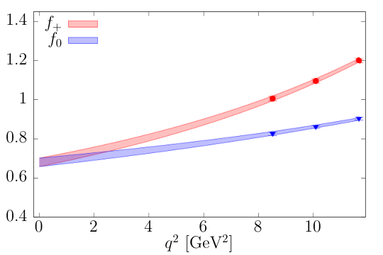
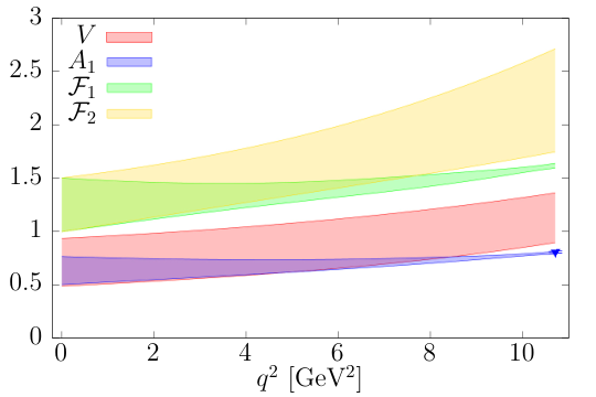
We perform the constrained multivariable fit by first randomly sampling values of the form factors for which lattice data is known. If correlations have been reported by the lattice QCD groups, they are implemented in the sampling. The preliminary HPQCD results for report only statistical error. To account for the unknown systematics like finite-volume and discretization effects, we include in quadrature an additional systematic error (as a percentage of the form factor at each point). Lines of best fit are then computed from the collection of sampled points using a least-squares procedure. The resulting form factors, exhibited with one- bands, are presented in Figs. 1–8. The for the form factors can be found in Table 3. Of particular note, our theoretical values for the form factors are consistent with those of the two processes for which experimental data has been obtained Aubert et al. 2010; Glattauer et al. 2016; Lees et al. 2019.
In interpreting these bands, it is important to recall that this analysis includes statistical errors from the lattice studies for which the notion of “” is well defined. However, the analysis also includes systematic errors for which, strictly speaking, it is not. Moreover, in assigning systematic error associated with limited lattice data for which systematic errors had not been carefully studied, or due to truncation errors in the theory, we have been quite conservative. Thus, one might reasonably expect the SM result to fall within these bands with a higher probability than had the bands been entirely due to statistical errors.
From Table 3, it is possible to investigate the convergence of BGL expansion. All the coefficients are consistent with zero at , suggesting that each series is rapidly converging; additional parameters are unnecessary at the present precision of lattice data. This lack of precision also allows for the parameters to fluctuate substantially, such that in a given fit each one can typically be , and therefore contribute significantly to the dispersive bounds of Eq. (29).
With this observation, one would expect the dispersive bounds to be saturated, similar to the results of Cohen et al. 2018b in which the dispersive bound for the unknown form factor was saturated. Fitting all seven processes together, Eq. (29) is typically saturated for all four channels (; ). However, this result occurs not only because the parameters are not well constrained. Surprisingly, Table 3 shows that for the two form factors , the coefficients are . Each one of them saturates about 25% of the dispersive bound. This result suggests that the inclusion of baryonic channels into the dispersive approach is particularly powerful.
In the case of , there are additional benefits beyond providing such a large contribution toward saturation. In the channel, only the and form factors contribute. At present, no lattice results for any exist. Given that form factors contribute significantly only to decays, this uncertainty is a sizeable fraction of the uncertainty in our predictions of . The large contribution of to the dispersive bound reduces this error. These dual benefits from including should motivate future efforts to obtain lattice results for form factors of other baryonic processes, i.e., .


| 7.2(1.0) | –17.(4) | 0.7(6) | ||
| 0.25(4) | –0.58(9) | 1(14) | ||
| 0.67(17) | –0.5(14) | 10(40) | ||
| 0.42(3) | –0.2(13) | 20(30) | ||
| 0.07(4) | –0.11(17) | 1(7) | ||
| 5.4(1.0) | –20(30) | –10(60) | ||
| 5.23(8) | –16(17) | 1(4) | ||
| 0.179(5) | –0.47(9) | –1.6(5) | ||
| 0.46(11) | 0(300) | 16(16) | ||
| 0.33(4) | –0.4(20) | 18(19) | ||
| 0.05(6) | –0.2(4) | 2(11) | ||
| 4(9) | –20(30) | 0(300) | ||
| 0.256(9) | –2.7(4) | 2(7) | ||
| 0.85(4) | –7.9(1.7) | 4(14) | ||
| 5.14(18) | –46(9) | 1(3) | ||
| 0.0613(18) | –0.49(9) | –1(3) | ||
| 0.356(12) | –2.7(5) | –3(4) | ||
| 5.23(18) | –53(9) | 1.3(1.2) | ||
| 6.1(6) | –30(30) | 10(70) | ||
| 0.18(3) | –0.8(7) | –3(15) | ||
| 0.47(9) | –2(3) | 20(60) | ||
| 0.34(5) | –2.6(2.0) | 40(60) | ||
| 0.058(10) | –0.3(3) | 9(8) | ||
| 4(10) | –21(16) | 0.8(9) |
In the case of , sufficient lattice data exists so that the constraint of heavy-quark symmetries is not required to fix the form factors. Therefore, we can use our results in that process to investigate how well the HQET relations are satisfied. While higher-order terms are known Bernlochner et al. 2018, we consider the leading-order relations in which the six form factors are all proportional to an Isgur-Wise function , which is typically expanded in powers of as
| (34) |
In this expansion, our results for the coefficients of the Taylor series are found in Table 4. One can see that our results, despite suggesting corrections to the HQET relations, are consistent with the sum-rule bounds: and Le Yaouanc et al. 2009.
In the final two rows of Table 4, we compute a pair of averages of the coefficients. The first, , is simply an average of parameters from all six form factors together, and would represent a best-fit phenomenological value for . The last row () instead averages over only and . This average is of interest because only these two form factors contribute appreciably to the differential decay rate of , the process measured by the LHCb Collaboration Aaij et al. 2017b. In that work, assuming the same leading-order HQET relations and the static approximation, LHCb extracted the values and from the decay . Good agreement is found between the LHCb results and those of . But if these results were used to make predictions far from , or for , then the other form factors begin to contribute appreciably, and a systematic error would be introduced because their corresponding coefficients differ dramatically from those of .
| 1.12(4) | 2.5(3) | 5.6(1.8) | |
| 1.51(7) | 3.3(5) | 8.0(1.8) | |
| 0.97(4) | 1.8(3) | 3.6(6) | |
| 0.90(3) | 1.7(3) | 3.4(1.8) | |
| 0.90(3) | 1.82(18) | 4.0(8) | |
| 1.02(4) | 2.2(3) | 4.8(6) | |
| 1.1(3) | 2.2(7) | 4(2) | |
| 0.90(3) | 1.7(2) | 3.6(1.4) |
Using the computed form factors, we extract three observables of experimental interest, and present the results in Table 5. The first is the semileptonic decay ratio:
| (35) |
For those for which existing theoretical values exist, we find good agreement. This result is to be expected, given that all the theoretical values rely at least in part upon the same lattice-QCD data used here. Beyond these checks, we have produced two new SM predictions, those of and , which can be compared to the upcoming LHCb results of Runs II and III. We find that the prediction is within of the current LHCb result of Aaij et al. 2018c.
The second observable is the polarization of the lepton, given by
| (36) |
where are the decay rates of a with fixed helicity . Only has been measured Hirose et al. 2017; Hirose et al. 2018 and our value agrees within uncertainties. For the other processes, we present predictions for comparison with future measurements.
The final observable we compute is the fractional longitudinal polarization of the decaying vector meson:
| (37) |
where is the decay rate of a vector with helicity . In the case of the , this quantity has been measured to be Abdesselam et al. 2019b, which is within of our result and other existing SM values Huang et al. 2018; Bhattacharya et al. 2019.
| 0.298(6) | 0.325(4) | — | |
| 0.252(14) | –0.51(5) | 0.45(3) | |
| 0.300(5) | 0.323(18) | — | |
| 0.20(3) | –0.49(5) | 0.44(5) | |
| 0.332(10) | –0.308(15) | — | |
| 0.30(5) | 0.33(11) | — | |
| 0.25(3) | –0.47(5) | 0.46(4) |


VII Discussion and Conclusion
In this work we have presented model-independent predictions of the hadronic transition form factors for the processes, , , , and , using a coupled global analysis. From these form factors, Standard-Model values for (- ratio), ( polarization), and ( longitudinal component) were computed. Also obtained, for the first time using this approach, are and . The near-term outlook for higher-statistics measurements from BELLE and LHCb, coupled with new lattice results, promise to reduce the uncertainty on the experimental and theoretical values dramatically, allowing for a refinement of the investigation of the charged-current anomalies. Additionally, new measurements like can be compared to our results to provide complementary constraints.
We have also derived nonzero recoil relations between the heavy-heavy meson form factors and the Isgur-Wise-like form factor at leading order in NRQCD. These results allow constraints on the slopes of unknown lattice form factors at to be obtained. Furthermore, these relations can be used as the basis of phenomenological models for the form factors.
The dominant sources of uncertainty in this analysis arise from the form factors for which no lattice data has been reported, all of which are in the processes. Upcoming results for Vaquero et al. 2019 and promise to provide insight into these form factors. The global analysis could also benefit from the inclusion of new processes. Given the large fractional saturation of the unitarity bounds by , the inclusion of could be particularly fruitful once such data is available.
Acknowledgements.
This work was supported by the U.S. Department of Energy under Contract No. DE-FG02-93ER-40762 (T.D.C. and H.L.) and the National Science Foundation under Grant No. PHY-1803912 (R.F.L.). H.L. acknowledges the hospitality of Arizona State University, where part of this work was performed.References
- Colangelo and De Fazio (2018) P. Colangelo and F. De Fazio, JHEP 06, 082 (2018), arXiv:1801.10468 [hep-ph] .
- Ivanov et al. (2016) M. A. Ivanov, J. G. Körner, and C.-T. Tran, Phys. Rev. D94, 094028 (2016), arXiv:1607.02932 [hep-ph] .
- Tran et al. (2018) C.-T. Tran, M. A. Ivanov, J. G. Körner, and P. Santorelli, Phys. Rev. D97, 054014 (2018), arXiv:1801.06927 [hep-ph] .
- Bhattacharya et al. (2016) S. Bhattacharya, S. Nandi, and S. K. Patra, Phys. Rev. D93, 034011 (2016), arXiv:1509.07259 [hep-ph] .
- Bhattacharya et al. (2017) S. Bhattacharya, S. Nandi, and S. K. Patra, Phys. Rev. D95, 075012 (2017), arXiv:1611.04605 [hep-ph] .
- Jaiswal et al. (2017) S. Jaiswal, S. Nandi, and S. K. Patra, JHEP 12, 060 (2017), arXiv:1707.09977 [hep-ph] .
- Bhattacharya et al. (2019) S. Bhattacharya, S. Nandi, and S. Kumar Patra, Eur. Phys. J. C79, 268 (2019), arXiv:1805.08222 [hep-ph] .
- Cohen et al. (2018a) T. D. Cohen, H. Lamm, and R. F. Lebed, Phys. Rev. D98, 034022 (2018a), arXiv:1807.00256 [hep-ph] .
- Bečirević et al. (2019) D. Bečirević, M. Fedele, I. Nišandžić, and A. Tayduganov, (2019), arXiv:1907.02257 [hep-ph] .
- Lees et al. (2012) J. P. Lees et al. (BaBar Collaboration), Phys. Rev. Lett. 109, 101802 (2012), arXiv:1205.5442 [hep-ex] .
- Lees et al. (2013) J. P. Lees et al. (BaBar Collaboration), Phys. Rev. D88, 072012 (2013), arXiv:1303.0571 [hep-ex] .
- Huschle et al. (2015) M. Huschle et al. (Belle Collaboration), Phys. Rev. D92, 072014 (2015), arXiv:1507.03233 [hep-ex] .
- Abdesselam et al. (2019a) A. Abdesselam et al. (Belle Collaboration), (2019a), arXiv:1904.08794 [hep-ex] .
- Sato et al. (2016) Y. Sato et al. (Belle Collaboration), Phys. Rev. D94, 072007 (2016), arXiv:1607.07923 [hep-ex] .
- Aaij et al. (2015) R. Aaij et al. (LHCb Collaboration), Phys. Rev. Lett. 115, 111803 (2015), [Erratum: Phys. Rev. Lett. 115, 159901 (2015)], arXiv:1506.08614 [hep-ex] .
- Hirose et al. (2017) S. Hirose et al. (Belle Collaboration), Phys. Rev. Lett. 118, 211801 (2017), arXiv:1612.00529 [hep-ex] .
- Aaij et al. (2018a) R. Aaij et al. (LHCb Collaboration), Phys. Rev. Lett. 120, 171802 (2018a), arXiv:1708.08856 [hep-ex] .
- Aaij et al. (2018b) R. Aaij et al. (LHCb Collaboration), Phys. Rev. D97, 072013 (2018b), arXiv:1711.02505 [hep-ex] .
- Hirose et al. (2018) S. Hirose et al. (Belle Collaboration), Phys. Rev. D97, 012004 (2018), arXiv:1709.00129 [hep-ex] .
- Amhis et al. (2017) Y. Amhis et al. (Heavy Flavor Averaging Group), Eur. Phys. J. C77, 895 (2017), updated results and plots available at https://hflav.web.cern.ch, arXiv:1612.07233 [hep-ex] .
- Bigi and Gambino (2016) D. Bigi and P. Gambino, Phys. Rev. D94, 094008 (2016), arXiv:1606.08030 [hep-ph] .
- Bernlochner et al. (2017) F. U. Bernlochner, Z. Ligeti, M. Papucci, and D. J. Robinson, Phys. Rev. D95, 115008 (2017), [Erratum: Phys. Rev. D97, 059902 (2018)], arXiv:1703.05330 [hep-ph] .
- Bigi et al. (2017) D. Bigi, P. Gambino, and S. Schacht, JHEP 11, 061 (2017), arXiv:1707.09509 [hep-ph] .
- Aaij et al. (2018c) R. Aaij et al. (LHCb Collaboration), Phys. Rev. Lett. 120, 121801 (2018c), arXiv:1711.05623 [hep-ex] .
- Cohen et al. (2018b) T. D. Cohen, H. Lamm, and R. F. Lebed, JHEP 09, 168 (2018b), arXiv:1807.02730 [hep-ph] .
- Aoki et al. (2019) S. Aoki et al. (Flavour Lattice Averaging Group), (2019), arXiv:1902.08191 [hep-lat] .
- Na et al. (2015) H. Na, C. M. Bouchard, G. P. Lepage, C. Monahan, and J. Shigemitsu (HPQCD Collaboration), Phys. Rev. D92, 054510 (2015), [Erratum: Phys. Rev. D93, 119906 (2016)], arXiv:1505.03925 [hep-lat] .
- Bailey et al. (2015) J. A. Bailey et al. (MILC Collaboration), Phys. Rev. D92, 034506 (2015), arXiv:1503.07237 [hep-lat] .
- McLean et al. (2019a) E. McLean, C. T. H. Davies, J. Koponen, and A. T. Lytle, (2019a), arXiv:1906.00701 [hep-lat] .
- Detmold et al. (2015) W. Detmold, C. Lehner, and S. Meinel, Phys. Rev. D92, 034503 (2015), arXiv:1503.01421 [hep-lat] .
- Bernlochner et al. (2018) F. U. Bernlochner, Z. Ligeti, D. J. Robinson, and W. L. Sutcliffe, Phys. Rev. Lett. 121, 202001 (2018), arXiv:1808.09464 [hep-ph] .
- Berns and Lamm (2018) A. Berns and H. Lamm, JHEP 12, 114 (2018), arXiv:1808.07360 [hep-ph] .
- Murphy and Soni (2018) C. W. Murphy and A. Soni, Phys. Rev. D98, 094026 (2018), arXiv:1808.05932 [hep-ph] .
- Cerri et al. (2018) A. Cerri et al., (2018), arXiv:1812.07638 [hep-ph] .
- (35) B. Hamilton and H. Jawahery, private communication.
- Boyd et al. (1995a) C. G. Boyd, B. Grinstein, and R. F. Lebed, Phys. Lett. B353, 306 (1995a), arXiv:hep-ph/9504235 [hep-ph] .
- Boyd et al. (1997) C. G. Boyd, B. Grinstein, and R. F. Lebed, Phys. Rev. D56, 6895 (1997), arXiv:hep-ph/9705252 [hep-ph] .
- Grinstein and Lebed (2015) B. Grinstein and R. F. Lebed, Phys. Rev. D92, 116001 (2015), arXiv:1509.04847 [hep-ph] .
- Colquhoun et al. (2016) B. Colquhoun, C. Davies, J. Koponen, A. Lytle, and C. McNeile (HPQCD Collaboration), Proceedings, 34th International Symposium on Lattice Field Theory (Lattice 2016): Southampton, UK, July 24–30, 2016, PoS LATTICE 2016, 281 (2016), arXiv:1611.01987 [hep-lat] .
- (40) A. Lytle, private communication.
- Wirbel et al. (1985) M. Wirbel, B. Stech, and M. Bauer, Z. Phys. C29, 637 (1985).
- Richman and Burchat (1995) J. D. Richman and P. R. Burchat, Rev. Mod. Phys. 67, 893 (1995), arXiv:hep-ph/9508250 [hep-ph] .
- Isgur and Wise (1989) N. Isgur and M. B. Wise, Phys. Lett. B232, 113 (1989).
- Isgur and Wise (1990) N. Isgur and M. B. Wise, Phys. Lett. B237, 527 (1990).
- Mannel et al. (1991) T. Mannel, W. Roberts, and Z. Ryzak, Nucl. Phys. B355, 38 (1991).
- Jenkins et al. (1993) E. E. Jenkins, M. E. Luke, A. V. Manohar, and M. J. Savage, Nucl. Phys. B390, 463 (1993), arXiv:hep-ph/9204238 [hep-ph] .
- Kiselev et al. (2000) V. V. Kiselev, A. K. Likhoded, and A. I. Onishchenko, Nucl. Phys. B569, 473 (2000), arXiv:hep-ph/9905359 [hep-ph] .
- Falk et al. (1990) A. F. Falk, H. Georgi, B. Grinstein, and M. B. Wise, Nucl. Phys. B343, 1 (1990).
- (49) V. V. Kiselev, arXiv:hep-ph/0211021 [hep-ph] .
- Bailey et al. (2014) J. A. Bailey et al. (Fermilab Lattice and MILC Collaborations), Phys. Rev. D89, 114504 (2014), arXiv:1403.0635 [hep-lat] .
- Harrison et al. (2018) J. Harrison, C. Davies, and M. Wingate (HPQCD Collaboration), Phys. Rev. D97, 054502 (2018), arXiv:1711.11013 [hep-lat] .
- McLean et al. (2019b) E. McLean, C. T. H. Davies, A. T. Lytle, and J. Koponen, Phys. Rev. D99, 114512 (2019b), arXiv:1904.02046 [hep-lat] .
- Boyd et al. (1995b) C. G. Boyd, B. Grinstein, and R. F. Lebed, Phys. Rev. Lett. 74, 4603 (1995b), arXiv:hep-ph/9412324 [hep-ph] .
- Boyd and Lebed (1997) C. G. Boyd and R. F. Lebed, Nucl. Phys. B485, 275 (1997), arXiv:hep-ph/9512363 [hep-ph] .
- Boyd et al. (1996) C. G. Boyd, B. Grinstein, and R. F. Lebed, Nucl. Phys. B461, 493 (1996), arXiv:hep-ph/9508211 [hep-ph] .
- Generalis (1990) S. C. Generalis, J. Phys. G16, 785 (1990).
- Reinders et al. (1980) L. J. Reinders, H. R. Rubinstein, and S. Yazaki, Phys. Lett. 97B, 257 (1980), [Erratum: Phys. Lett. 100B, 519 (1981)].
- Reinders et al. (1981) L. J. Reinders, S. Yazaki, and H. R. Rubinstein, Phys. Lett. 103B, 63 (1981).
- Reinders et al. (1985) L. J. Reinders, H. Rubinstein, and S. Yazaki, Phys. Rept. 127, 1 (1985).
- Djouadi and Gambino (1994) A. Djouadi and P. Gambino, Phys. Rev. D49, 3499 (1994), [Erratum: Phys. Rev. D53, 4111 (1996)], arXiv:hep-ph/9309298 [hep-ph] .
- Aaij et al. (2017a) R. Aaij et al. (LHCb Collaboration), Phys. Rev. D95, 032005 (2017a), arXiv:1612.07421 [hep-ex] .
- Sirunyan et al. (2019) A. M. Sirunyan et al. (CMS Collaboration), Phys. Rev. Lett. 122, 132001 (2019), arXiv:1902.00571 [hep-ex] .
- Eichten and Quigg (2019) E. J. Eichten and C. Quigg, Phys. Rev. D99, 054025 (2019), arXiv:1902.09735 [hep-ph] .
- Aubert et al. (2010) B. Aubert et al. (BaBar Collaboration), Phys. Rev. Lett. 104, 011802 (2010), arXiv:0904.4063 [hep-ex] .
- Glattauer et al. (2016) R. Glattauer et al. (Belle Collaboration), Phys. Rev. D93, 032006 (2016), arXiv:1510.03657 [hep-ex] .
- Lees et al. (2019) J. P. Lees et al. (BaBar Collaboration), Phys. Rev. Lett. 123, 091801 (2019), arXiv:1903.10002 [hep-ex] .
- Le Yaouanc et al. (2009) A. Le Yaouanc, L. Oliver, and J.-C. Raynal, Phys. Rev. D79, 014023 (2009), arXiv:0808.2983 [hep-ph] .
- Aaij et al. (2017b) R. Aaij et al. (LHCb Collaboration), Phys. Rev. D96, 112005 (2017b), arXiv:1709.01920 [hep-ex] .
- Abdesselam et al. (2019b) A. Abdesselam et al. (Belle Collaboration), in 10th International Workshop on the CKM Unitarity Triangle (CKM 2018) Heidelberg, Germany, September 17-21, 2018 (2019) arXiv:1903.03102 [hep-ex] .
- Huang et al. (2018) Z.-R. Huang, Y. Li, C.-D. Lu, M. A. Paracha, and C. Wang, Phys. Rev. D98, 095018 (2018), arXiv:1808.03565 [hep-ph] .
- Vaquero et al. (2019) A. Vaquero, C. DeTar, A. X. El-Khadra, A. S. Kronfeld, J. Laiho, and R. S. Van de Water, in 17th Conference on Flavor Physics and CP Violation (FPCP 2019) Victoria, BC, Canada, May 6-10, 2019 (2019) arXiv:1906.01019 [hep-lat] .