跳到论文正文
W Papers独立论文阅读器 arXiv:1909.10439 论文正文 计算阅读时间 · 0%
引用这篇论文根据当前论文元数据生成,正式投稿前建议核对。


License: arXiv.org perpetual non-exclusive license
arXiv:1909.10439v4 [math.PR] 21 Apr 2021

Quantitative homogenization of the parabolic and elliptic Green’s functions on percolation clusters

Paul Dario P. DarioSchool of Mathematical Sciences, Tel Aviv University, Ramat Aviv, Tel Aviv 69978, Israel Email address: pauldario@mail.tau.ac.il and Chenlin Gu C. GuDMA, Ecole normale supérieure, PSL Research University, Paris, France Email address: chenlin.gu@ens.fr
Date: August 11, 2026
Abstract.

We study the heat kernel and the Green’s function on the infinite supercritical percolation cluster in dimension d≥2d\geq 2 and prove a quantitative homogenization theorem for these functions with an almost optimal rate of convergence. These results are a quantitative version of the local central limit theorem proved by Barlow and Hambly in [23]. The proof relies on a structure of renormalization for the infinite percolation cluster introduced in [12], Gaussian bounds on the heat kernel established by Barlow in [21] and tools of the theory of quantitative stochastic homogenization. An important step in the proof is to establish a C0,1C^{0,1}-large-scale regularity theory for caloric functions on the infinite cluster and is of independent interest.

Key words and phrases: 
Stochastic homogenization, local central limit theorem, parabolic equation, large-scale regularity, supercritical percolation
2010 Mathematics Subject Classification
35B27, 60K37, 60K35
Refer to caption
Refer to caption
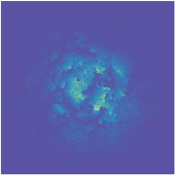
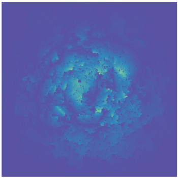
Figure 1. The figure on the left represents the density distribution of the function td2​p​(t,⋅,0)t^{\frac{d}{2}}p(t,\cdot,0) where the map pp is the 2-dimensional heat kernel on the infinite percolation cluster with probability 𝔭=0.7\mathfrak{p}=0.7 at time t=1000t=1000; it is similar to a Gaussian distribution. The figure on the right is the error between the map td2​p​(t,⋅,0)t^{\frac{d}{2}}p(t,\cdot,0) and the normalized Gaussian heat kernel θ​(p)−1​td2​p¯​(t,⋅)\theta(p)^{-1}t^{\frac{d}{2}}\bar{p}(t,\cdot) defined in (1.5); it is small compared to density distribution on the left.

1. Introduction

1.1. General introduction and main results

In this article, we study the continuous-time random walk on the infinite cluster of the supercritical Bernoulli bond percolation of the Euclidean lattice ℤd\mathbb{Z}^{d}, in dimension d≥2d\geq 2. The model considered is a specific case of the general random conductance model and can be described as follows. We let ℬd\mathcal{B}_{d} be the set of bonds of ℤd\mathbb{Z}^{d}, i.e., the set of unordered pairs of nearest neighbors of ℤd\mathbb{Z}^{d}. We denote by Ω\Omega the set of functions from ℬd\mathcal{B}_{d} to the set of non-negative real numbers [0,∞)[0,\infty). A generic element of Ω\Omega is denoted by 𝐚\mathbf{a} and called an environment.

For a given environment 𝐚∈Ω\mathbf{a}\in\Omega and a given bond e∈ℬde\in\mathcal{B}_{d}, we call the value 𝐚⁡(e)\mathbf{a}(e) the conductance of the bond ee. We fix an ellipticity parameter λ∈(0,1]\lambda\in(0,1] and add some randomness to the model by assuming that the collection of conductances {𝐚⁡(e)}e∈ℬd\left\{\mathbf{a}(e)\right\}_{e\in\mathcal{B}_{d}} is an i.i.d. family of random variables whose law is supported in the set {0}∪[λ,1]\{0\}\cup[\lambda,1]. We define 𝔭:=ℙ[𝐚(e)≠0]\mathfrak{p}:=\mathbb{P}\left[\mathbf{a}(e)\neq 0\right] and assume that

𝔭>𝔭c​(d),\mathfrak{p}>\mathfrak{p}_{c}(d),

where 𝔭c​(d)\mathfrak{p}_{c}(d) is the bond percolation threshold for the lattice ℤd\mathbb{Z}^{d}. This assumption ensures that, almost surely, there exists a unique infinite connected component of edges with non-zero conductances (or cluster) which we denote by 𝒞∞\mathscr{C}_{\infty} (see [35]). This cluster has a non-zero density which is given by the probability θ(𝔭):=ℙ[0∈𝒞∞]\theta(\mathfrak{p}):=\mathbb{P}\left[0\in\mathscr{C}_{\infty}\right]. The model of continuous-time random walk considered in this article is the variable speed random walk (or VSRW) and is defined as follows. Given an environment 𝐚∈Ω\mathbf{a}\in\Omega and a starting point y∈𝒞∞y\in\mathscr{C}_{\infty}, we endow each edge e∈ℬde\in\mathcal{B}_{d} with a random clock whose law is exponential of parameter 𝐚⁡(e)\mathbf{a}(e) and assume that they are mutually independent. We then let (Xt)t≥0\left(X_{t}\right)_{t\geq 0} be the random walk which starts from yy, i.e., X0=yX_{0}=y, and, when X⁡(t)=xX(t)=x, the random walker waits at xx until one of the clocks at an adjacent edge to xx rings, and moves across the edge to the neighboring point instantly. We then restart the clocks. This construction gives rise to a continuous-time Markov process on the infinite cluster 𝒞∞\mathscr{C}_{\infty} whose generator is the elliptic operator ∇⋅𝐚∇\nabla\cdot\mathbf{a}\nabla defined by, for each function u:𝒞∞→ℝu:\mathscr{C}_{\infty}\rightarrow\mathbb{R} and each point x∈𝒞∞x\in\mathscr{C}_{\infty},

(1.1) ∇⋅𝐚∇u(x):=∑z∼x𝐚({x,z})(u(z)−u(x)).\nabla\cdot\mathbf{a}\nabla u(x):=\sum_{z\sim x}\mathbf{a}(\{x,z\})\left(u(z)-u(x)\right).

We denote the transition density of the random walk by

p⁡(t,x,y)=p𝐚​(t,x,y):=ℙy𝐚​(Xt=x),p\left(t,x,y\right)=p^{\mathbf{a}}\left(t,x,y\right):=\mathbb{P}^{\mathbf{a}}_{y}\left(X_{t}=x\right),

and often omit the dependence in the environment 𝐚\mathbf{a} in the notation. The transition density can be equivalently defined as the solution of the parabolic equation

(1.2) {∂tp(⋅,⋅,y)−∇⋅𝐚∇p(⋅,⋅,y)=0in​(0,∞)×𝒞∞,p⁡(0,⋅,y)=δyin​𝒞∞.\left\{\begin{array}[]{cc}\partial_{t}p(\cdot,\cdot,y)-\nabla\cdot\mathbf{a}\nabla p(\cdot,\cdot,y)=0&~\mbox{in}~(0,\infty)\times\mathscr{C}_{\infty},\\ p(0,\cdot,y)=\delta_{y}&~\mbox{in}~\mathscr{C}_{\infty}.\end{array}\right.

Due to this characterization, we often refer to the transition density pp as the heat kernel or the parabolic Green’s function.

There are other related models of random walk on supercritical percolation clusters which have been studied in the literature, two of the most common ones are:

  1. (i)

    The constant speed random walk (or CSRW), the random walker starts from a point y∈𝒞∞y\in\mathscr{C}_{\infty}. When X⁡(t)=xX(t)=x, it waits for an exponential time of parameter 11 and then jumps to a neighboring point zz according to the transition probability

    (1.3) P⁡(x,z)=𝐚⁡({x,z})∑w∼x𝐚⁡({x,w}).P(x,z)=\frac{\mathbf{a}\left(\{x,z\}\right)}{\sum_{w\sim x}\mathbf{a}\left(\{x,w\}\right)}.

    This construction also gives rise to a continuous-time Markov process whose generator is given by, for each function u:𝒞∞→ℝu:\mathscr{C}_{\infty}\to\mathbb{R} and each point y∈𝒞∞y\in\mathscr{C}_{\infty},

    1∑z∼x𝐚⁡({x,z})​∑z∼x𝐚⁡({x,z})​(u⁡(z)−u⁡(x)).\frac{1}{\sum_{z\sim x}\mathbf{a}\left(\{x,z\}\right)}\sum_{z\sim x}\mathbf{a}(\{x,z\})\left(u(z)-u(x)\right).
  2. (ii)

    The simple random walk (or SRW), the random walk (Xn)n∈ℕ\left(X_{n}\right)_{n\in\mathbb{N}} is indexed on the integers, it starts from a point y∈𝒞∞y\in\mathscr{C}_{\infty}, when Xn=xX_{n}=x, the value of Xn+1X_{n+1} is chosen randomly among all the neighbors of xx following the transition probability (1.3).

These processes have similar, although not identical, properties and have been the subject of interest in the literature. In the case of the percolation cluster, i.e., when the environment 𝐚\mathbf{a} is only allowed to take the values 00 or 11, an annealed invariance principle was proved in [42] by De Masi, Ferrari, Goldstein and Wick. In [80], Sidoravicius and Sznitman proved a quenched invariance principle for the simple random walk in dimension d≥4d\geq 4. This result was extended to every dimension d≥2d\geq 2 by Berger and Biskup in [28] (for the SRW) and by Mathieu and Piatnitski in [69] (for the CSRW).

For the VSRW, a similar quenched invariance principle holds: there exists a deterministic diffusivity constant σ¯>0\bar{\sigma}>0 such that, for almost every environment, the following convergence holds in the Skorokhod topology

(1.4) ε​X⋅ε2​⟶ε→0(law)​σ¯​B⋅,\varepsilon X_{\frac{\cdot}{\varepsilon^{2}}}\overset{\mathrm{(law)}}{\underset{\varepsilon\rightarrow 0}{\longrightarrow}}\bar{\sigma}B_{\cdot},

where B⋅B_{\cdot} is a standard Brownian motion. From a homogenization perspective, the diffusivity σ¯2\bar{\sigma}^{2} of the limiting Brownian motion is related to the homogenized coefficient 𝐚﹇{\overbracket{\mathbf{a}}} associated to the elliptic and parabolic problems on the percolation cluster by the identity 𝐚﹇=12​θ​(𝔭)​σ¯2{\overbracket{\mathbf{a}}}=\frac{1}{2}\theta(\mathfrak{p})\bar{\sigma}^{2} (see the formula (B.5) of Appendix B).

The properties of the heat kernel pp on the infinite cluster have been investigated in the literature. In [70], Mathieu and Remy proved that, almost surely, the heat kernel decays as fast as t−d/2t^{-d/2}. These bounds were extended in [21] by Barlow who established Gaussian lower and upper bounds for this function; we will recall his precise result in Theorem 4 below.

In the article [23], Barlow and Hambly proved a parabolic Harnack inequality, a local central limit theorem for the CSRW, and bounds on the elliptic Green’s function on the infinite cluster. Their main result can be adapted to the case of the VSRW, and reads as follows: if we define, for each t≥0t\geq 0 and x∈ℝdx\in{\mathbb{R}^{d}},

(1.5) p¯​(t,x):=1(2​π​σ¯2​t)d/2​exp⁡(−|x|22​σ¯2​t),\bar{p}(t,x):=\frac{1}{\left(2\pi\bar{\sigma}^{2}t\right)^{d/2}}\exp\left(-\frac{|x|^{2}}{2\ \bar{\sigma}^{2}t}\right),

the heat kernel with diffusivity σ¯\bar{\sigma}, then, for each time T>0T>0, the following convergence holds, ℙ\mathbb{P}-almost surely on the event {0∈𝒞∞}\{0\in\mathscr{C}_{\infty}\},

(1.6) limn→∞|nd/2​p​(n​t,gnω​(x),0)−θ​(𝔭)−1​p¯​(t,x)|=0,\lim_{n\to\infty}\left|n^{d/2}p(nt,g^{\omega}_{n}(x),0)-\theta(\mathfrak{p})^{-1}\bar{p}(t,x)\right|=0,

uniformly in the spatial variable x∈ℝdx\in{\mathbb{R}^{d}} and in the time variable t≥Tt\geq T, where the notation gnω​(x)g^{\omega}_{n}(x) means the closest point to n​x\sqrt{n}x in the infinite cluster under the environment ω\omega.

The main result of this article is a quantitative version of the local central limit theorem for the VSRW and is stated below.

Theorem 1.

For each exponent δ>0\delta>0, there exist a positive constant C<∞C<\infty and an exponent s>0s>0, depending only on the parameters d,λ,𝔭d,\lambda,\mathfrak{p} and δ\delta, such that for every y∈ℤdy\in\mathbb{Z}^{d}, there exists a non-negative random time 𝒯par,δ​(y)\mathcal{T}_{\mathrm{par},\delta}(y) satisfying the stochastic integrability estimate

∀T≥0,ℙ⁡(𝒯par,δ​(y)≥T)≤C​exp⁡(−TsC),\forall T\geq 0,~\mathbb{P}\left(\mathcal{T}_{\mathrm{par},\delta}(y)\geq T\right)\leq C\exp\left(-\frac{T^{s}}{C}\right),

such that, on the event {y∈𝒞∞}\{y\in\mathscr{C}_{\infty}\}, for every x∈𝒞∞x\in\mathscr{C}_{\infty} and every t≥max⁡(𝒯par,δ​(y),|x−y|)t\geq\max\left(\mathcal{T}_{\mathrm{par},\delta}(y),|x-y|\right),

(1.7) |p⁡(t,x,y)−θ​(𝔭)−1​p¯​(t,x−y)|≤C​t−d2−(12−δ)​exp⁡(−|x−y|2C​t).\left|p(t,x,y)-\theta(\mathfrak{p})^{-1}\bar{p}(t,x-y)\right|\leq Ct^{-\frac{d}{2}-\left(\frac{1}{2}-\delta\right)}\exp\left(-\frac{|x-y|^{2}}{Ct}\right).
Remark 1.1.

The heat kernel pp does not exactly converge to the heat kernel p¯\bar{p} and there is an additional normalization constant θ​(𝔭)−1\theta(\mathfrak{p})^{-1} in (1.7). A heuristic reason explaining why such a term is necessary is the following: since p⁡(t,⋅,y)p(t,\cdot,y) is a probability measure on the infinite cluster, one has

∑x∈𝒞∞p⁡(t,x,y)=1.\sum_{x\in\mathscr{C}_{\infty}}p\left(t,x,y\right)=1.

One also has, by definition of the heat kernel p¯\bar{p},

∫ℝdp¯​(t,x−y)​𝑑x=1.\int_{{\mathbb{R}^{d}}}\bar{p}(t,x-y)\,dx=1.

Since the infinite cluster has density θ⁡(𝔭)\theta(\mathfrak{p}), we expect that

∑x∈𝒞∞p¯​(t,x−y)≃θ⁡(𝔭)​∫ℝdp¯​(t,x−y)​𝑑x=θ⁡(𝔭),\sum_{x\in\mathscr{C}_{\infty}}\bar{p}(t,x-y)\simeq\theta(\mathfrak{p})\int_{{\mathbb{R}^{d}}}\bar{p}(t,x-y)\,dx=\theta(\mathfrak{p}),

and we refer to Proposition A.7 for a precise statement. As a consequence, we cannot expect the maps pp and p¯\bar{p} to be close since they have different mass on the infinite cluster; adding the normalization term θ​(𝔭)−1\theta(\mathfrak{p})^{-1} ensures that the mass of θ​(𝔭)−1​p¯\theta(\mathfrak{p})^{-1}\bar{p} on the infinite cluster is approximately equal to 11.

As an application of this result, we deduce a quantitative homogenization theorem for the elliptic Green’s function on the infinite cluster. In dimension d≥3d\geq 3, given an environment 𝐚∈Ω\mathbf{a}\in\Omega and a point y∈𝒞∞y\in\mathscr{C}_{\infty}, we define the Green’s function g⁡(⋅,y)g(\cdot,y) as the solution of the equation

−∇⋅𝐚∇g(⋅,y)=δyin𝒞∞such thatg(x,y)⟶x→∞0.-\nabla\cdot\mathbf{a}\nabla g(\cdot,y)=\delta_{y}~\mbox{in}~\mathscr{C}_{\infty}~\mbox{such that}~g(x,y)\underset{x\rightarrow\infty}{\longrightarrow}0.

This function exists, is unique almost surely and is related to the transition probability pp through the identity

(1.8) g⁡(x,y)=∫0∞p⁡(t,x,y)​𝑑t.g(x,y)=\int_{0}^{\infty}p(t,x,y)\,dt.

In dimension 22, the situation is different since the Green’s function is not bounded at infinity, and we define g⁡(⋅,y)g\left(\cdot,y\right) as the unique function which satisfies

−∇⋅𝐚∇g(⋅,y)=δyin𝒞∞,1|x|g(x,y)⟶x→∞0andg(y,y)=0.-\nabla\cdot\mathbf{a}\nabla g(\cdot,y)=\delta_{y}~\mbox{in}~\mathscr{C}_{\infty},~\frac{1}{|x|}g(x,y)\underset{x\rightarrow\infty}{\longrightarrow}0~\mbox{and}~g(y,y)=0.

This function is related to the transition probability pp through the identity

g⁡(x,y)=∫0∞(p⁡(t,x,y)−p⁡(t,y,y))​𝑑t.g(x,y)=\int_{0}^{\infty}\left(p(t,x,y)-p(t,y,y)\right)\,dt.

In the statement below, we denote by g¯\bar{g} the homogenized Green’s function defined by the formula, for each point x∈ℝd∖{0}x\in{\mathbb{R}^{d}}\setminus\left\{0\right\},

(1.9) g¯​(x):={−1π​σ¯2​θ​(𝔭)​ln⁡|x|if​d=2,Γ⁡(d/2−1)(2​πd/2​σ¯2​θ​(𝔭))​1|x|d−2if​d≥3,\bar{g}(x):=\left\{\begin{array}[]{lcl}-\frac{1}{\pi\bar{\sigma}^{2}\theta(\mathfrak{p})}\ln\left|x\right|&\hskip 14.22636pt\mbox{if}~d=2,\\ \frac{\Gamma\left(d/2-1\right)}{\left(2\pi^{d/2}\bar{\sigma}^{2}\theta(\mathfrak{p})\right)}\frac{1}{|x|^{d-2}}&\hskip 14.22636pt\mbox{if}~d\geq 3,\end{array}\right.

where the symbol Γ\Gamma denotes the standard Gamma function. Theorem 2 describes the asymptotic behavior of the Green’s function gg.

Theorem 2.

For each exponent δ>0\delta>0, there exist a positive constant C<∞C<\infty and an exponent s>0s>0, depending only on the parameters d,λ,𝔭d,\lambda,\mathfrak{p} and δ\delta, such that for every y∈ℤdy\in\mathbb{Z}^{d}, there exists a non-negative random variable ℳell,δ​(y)\mathcal{M}_{\mathrm{ell},\delta}(y) satisfying

∀R≥0,ℙ⁡(ℳell,δ​(y)≥R)≤C​exp⁡(−RsC),\forall R\geq 0,~\mathbb{P}\left(\mathcal{M}_{\mathrm{ell},\delta}(y)\geq R\right)\leq C\exp\left(-\frac{R^{s}}{C}\right),

such that, on the event {y∈𝒞∞}\{y\in\mathscr{C}_{\infty}\}:

  1. (1)

    In dimension d≥3d\geq 3, for every point x∈𝒞∞x\in\mathscr{C}_{\infty} satisfying |x−y|≥ℳell,δ​(y)|x-y|\geq\mathcal{M}_{\mathrm{ell},\delta}(y),

    (1.10) |g⁡(x,y)−g¯​(x−y)|≤1|x−y|1−δ​C|x−y|d−2.\left|g(x,y)-\bar{g}(x-y)\right|\leq\frac{1}{|x-y|^{1-\delta}}\frac{C}{|x-y|^{d-2}}.
  2. (2)

    In dimension 22, the limit

    K⁡(y):=limx→∞(g⁡(x,y)−g¯​(x−y)),K(y):=\lim_{x\rightarrow\infty}\left(g(x,y)-\bar{g}(x-y)\right),

    exists, is finite almost surely and satisfies the stochastic integrability estimate

    ∀R≥0,ℙ⁡(|K⁡(y)|≥R)≤C​exp⁡(−RsC).\forall R\geq 0,~\mathbb{P}\left(|K(y)|\geq R\right)\leq C\exp\left(-\frac{R^{s}}{C}\right).

    Moreover, for every point x∈𝒞∞x\in\mathscr{C}_{\infty} satisfying |x−y|≥ℳell,δ​(y)|x-y|\geq\mathcal{M}_{\mathrm{ell},\delta}(y),

    (1.11) |g⁡(x,y)−g¯​(x−y)−K⁡(y)|≤C|x−y|1−δ.\left|g(x,y)-\bar{g}(x-y)-K(y)\right|\leq\frac{C}{|x-y|^{1-\delta}}.
Remark 1.2.

In dimension 22, the situation is specific due to the unbounded behavior of the Green’s function, and the theorem identifies the first-order term. The second term in the asymptotic development is of constant order and is random: with the normalization chosen for the Green’s function, the constant KK depends on the geometry of the infinite cluster and cannot be deterministic. We nevertheless expect it not to be too large and prove that it satisfies a stretched exponential stochastic integrability estimate.

Refer to caption
Refer to caption
Refer to caption
Refer to caption
Refer to caption
Refer to caption
Refer to caption
Refer to caption
Refer to caption
Refer to caption
Refer to caption
Refer to caption
Refer to caption
Refer to caption
Refer to caption
Figure 2. A simulation to illustrate the convergence of the parabolic Green’s function for the VSRW on the infinite cluster with 𝔭=0.6\mathfrak{p}=0.6. We use different colors to represent the level sets of the map td2​p​(t,⋅,y)t^{\frac{d}{2}}p(t,\cdot,y) in the first two rows. The figures in first row are drawn for the short times t=100,200,300,400,500t=100,200,300,400,500 in a cube of size 64×6464\times 64 and the level sets of the heat kernel are perturbed by the geometry of the infinite cluster. In the second row, the figures are drawn for the long times t=500,1000,2000,3000,4000t=500,1000,2000,3000,4000 and in a cube of size 256×256256\times 256; in this case, homogenization happens and the geometry of the level sets of the heat kernel is similar to the one of a Gaussian heat kernel. In the third row, we simulate the function td2|p(t,⋅,y)−θ(𝔭)−1p¯(t,⋅−y)|𝟙{x∈𝒞∞}t^{\frac{d}{2}}\left|p(t,\cdot,y)-\theta(\mathfrak{p})^{-1}\bar{p}(t,\cdot-y)\right|\mathds{1}_{\{x\in\mathscr{C}_{\infty}\}} associated to the figures in the second line and we observe that the errors decay to 00 as the time tends to infinity.

We complete this section by mentioning a potential application of these theorems. Theorem 1 shows that the law of the VSRW on the infinite percolation cluster converges quantitatively to the one of the Brownian motion (σ¯​Bt)t≥0\left(\bar{\sigma}B_{t}\right)_{t\geq 0}. To go one step further in the analysis, one can try to construct a coupling between the random walk (Xt)t≥0(X_{t})_{t\geq 0} and the Brownian motion (σ¯​Bt)t≥0\left(\bar{\sigma}B_{t}\right)_{t\geq 0} such that their trajectories are close, i.e., such that sup0≤s≤t|Xs−σ¯​Bs|\sup_{0\leq s\leq t}|X_{s}-\bar{\sigma}B_{s}| is small. This question is known as the embedding problem: a good error should be at least of order o⁡(t)o(\sqrt{t}). In the case of the simple random walk on ℤd\mathbb{Z}^{d}, the optimal result is given by the Komlós-Major-Tusnády Approximation (see [64, 65]) and gives an error of order O⁡(log⁡t)O(\log t). Adapting this result to the setting considered here requires to take into account the degenerate geometry of the percolation cluster; we believe that Theorem 1 can be useful in this regard.

1.2. Strategy of the proof

On the supercritical percolation cluster, a qualitative version of Theorem 1 is established by Barlow and Hambly in [23], where the strategy implemented is to first prove a parabolic Harnack inequality for the heat equation. From the Harnack inequality, one derives a C0,αC^{0,\alpha}-Hölder regularity estimate (for some small exponent α>0\alpha>0) on the heat kernel. It is then possible to combine this additional regularity with the quenched invariance principle, established on the percolation cluster in [80, 70, 28], to obtain the local central limit theorem.

In the present article, the strategy adopted is different and follows ideas from the theory of stochastic homogenization, more specifically the ones of [15, Chapter 8]. A first crucial ingredient in the proof is the first-order corrector, which can be characterized as follows: given a slope p∈ℝdp\in{\mathbb{R}^{d}}, the corrector χp\chi_{p} is defined as the unique function (up to a constant) which is a solution of the elliptic equation

−∇⋅𝐚(p+∇χp)=0in𝒞∞,-\nabla\cdot\mathbf{a}\left(p+\nabla\chi_{p}\right)=0~\mbox{in}~\mathscr{C}_{\infty},

and which has sublinear oscillation, i.e.,

1r​oscx∈𝒞∞∩Brχp:=1r​(supx∈𝒞∞∩Brχp−infx∈𝒞∞∩Brχp)​⟶r→∞​0.\frac{1}{r}\osc_{x\in\mathscr{C}_{\infty}\cap B_{r}}\chi_{p}:=\frac{1}{r}\left(\sup_{x\in\mathscr{C}_{\infty}\cap B_{r}}\chi_{p}-\inf_{x\in\mathscr{C}_{\infty}\cap B_{r}}\chi_{p}\right)\underset{r\rightarrow\infty}{\longrightarrow}0.

The corrector is defined and some of its important properties are presented in Section 2.3. We note that the use of the corrector to study random walk on supercritical percolation cluster is not new: it is a key ingredient in the proofs of the quenched invariance principle (see [80, 70, 28]). Once equipped with this function, the analysis relies on a classical strategy in stochastic homogenization: the two-scale expansion. The general approach relies on the definition of the function

(1.12) h⁡(t,x,y):=θ​(𝔭)−1​(p¯​(t,x−y)+∑k=1d∂kp¯​(t,x−y)​χek​(x)),h(t,x,y):=\theta(\mathfrak{p})^{-1}\left(\bar{p}\left(t,x-y\right)+\sum_{k=1}^{d}\partial_{k}\bar{p}(t,x-y)\chi_{e_{k}}(x)\right),

where (ek)k={1,⋯,d}\left(e_{k}\right)_{k=\{1,\cdots,d\}} denotes the canonical basis of ℝd{\mathbb{R}^{d}} and p¯\bar{p} is the continuous heat kernel defined in (1.5). The strategy is then to compute the value of

(1.13) ∂th−∇⋅𝐚∇h,\partial_{t}h-\nabla\cdot\mathbf{a}\nabla h,

by using the explicit formula on hh stated in (1.12) and to prove that it is quantitatively small in the correct functional space (precisely, the parabolic H¯−1\underline{H}^{-1} space introduced in (1.33)). Obtaining this result requires two types of quantitative information on the corrector:

  • •

    One needs to have quantitative sublinearity of the corrector, i.e.,

    (1.14) 1rα​oscx∈𝒞∞∩Brχp​⟶r→∞​0,\frac{1}{r^{\alpha}}\osc_{x\in\mathscr{C}_{\infty}\cap B_{r}}\chi_{p}\underset{r\rightarrow\infty}{\longrightarrow}0,

    for every exponent α>0\alpha>0.

  • •

    One needs to have a quantitative control on the flux of the corrector in the weak H¯−1\underline{H}^{-1} norm,

    (1.15) 1rα​‖𝐚⁡(p+∇χp)−12​σ¯2​p‖H¯−1​(𝒞∞∩Br)​⟶r→∞​0,\frac{1}{r^{\alpha}}\left\|\mathbf{a}\left(p+\nabla\chi_{p}\right)-\frac{1}{2}\bar{\sigma}^{2}p\right\|_{\underline{H}^{-1}(\mathscr{C}_{\infty}\cap B_{r})}\underset{r\rightarrow\infty}{\longrightarrow}0,

    for every exponent α>0\alpha>0, where σ¯2\bar{\sigma}^{2} is the same diffusivity constant as in the definition (1.5) of the heat kernel p¯\bar{p}.

The sublinearity of the corrector in the setting of the percolation cluster is established qualitatively in [80, 70, 28] and quantitatively in [12, 40, 62]. The second property (1.15) cannot be directly deduced from the results of [12, 40, 62] and Appendix B is devoted to the proof of this result.

Once one has good quantitative control over the H¯−1\underline{H}^{-1}-norm of ∂th−∇⋅𝐚∇h\partial_{t}h-\nabla\cdot\mathbf{a}\nabla h, the proof of the result follows from the following two arguments:

  1. (i)

    First, one shows that the function hh is (quantitatively) close to the function θ−1​(𝔭)​p¯\theta^{-1}(\mathfrak{p})\bar{p}. This is achieved by proving that the second term in the right side of (1.12) is small and relies on the quantitative sublinearity of the corrector stated in (1.14).

  2. (ii)

    Second, one needs to show that the function hh is (quantitatively) close to the heat kernel pp. To prove this, the strategy is to use that the map pp solves the parabolic equation

    ∂tp−∇⋅𝐚∇p=0,\partial_{t}p-\nabla\cdot\mathbf{a}\nabla p=0,

    and subtract it from (1.13) to obtain that ∂t(p−h)−∇⋅𝐚∇(p−h)\partial_{t}(p-h)-\nabla\cdot\mathbf{a}\nabla(p-h) is small in the H¯−1\underline{H}^{-1} norm. We then use the function (p−h)(p-h) as a test function in the previous equation, to deduce that (p−h)(p-h) has to be small in the H1H^{1}-norm.

This strategy is essentially carried out in Section 4.2. Nevertheless, a number of difficulties have to be treated in order to implement it. They are mainly due to three distinct causes which are listed below.

First, the heat kernel pp has an initial condition at time t=0t=0 which is a Dirac (see the equation (1.2)). It is rather singular and causes serious troubles in the analysis. To fix this issue, one replaces the initial condition in (1.2) by a function which is smoother, but which is still a good approximation of the Dirac function. The argument is sketched in the following paragraph. We fix a large time t>0t>0 and want to prove the main estimate (1.7) for this particular time tt. To this end, we replace the initial condition δy\delta_{y} by the function p¯(τ,⋅−y)\bar{p}(\tau,\cdot-y) for some time τ≪t\tau\ll t, and we define

(1.16) {∂tq−∇⋅(𝐚∇q)=0in​(τ,∞)×𝒞∞,q(τ,⋅,y)=θ(𝔭)−1p¯(τ,⋅−y)on​𝒞∞.\left\{\begin{array}[]{lcl}\partial_{t}q-\nabla\cdot\left(\mathbf{a}\nabla q\right)=0&\mbox{in}~(\tau,\infty)\times\mathscr{C}_{\infty},\\ q(\tau,\cdot,y)=\theta(\mathfrak{p})^{-1}\bar{p}(\tau,\cdot-y)&\mbox{on}~\mathscr{C}_{\infty}.\end{array}\right.

The strategy is then to make the following compromise: we want to choose the coefficient τ\tau small enough (in particular, much smaller than tt) so that the initial data p¯(τ,⋅−y)\bar{p}(\tau,\cdot-y) is close to the Dirac function δy\delta_{y}, the objective being that the function q⁡(t,⋅,y)q(t,\cdot,y) is close to p⁡(t,⋅,y)p(t,\cdot,y) (see Lemma 4.1); we also want to choose τ\tau large enough so that the initial data p¯​(τ,⋅)\bar{p}(\tau,\cdot) is smooth enough. Our choice will be τ=t1−κ\tau=t^{1-\kappa} for some small exponent κ>0\kappa>0. This approach is essentially the subject of Section 4.1.

The second difficulty is that the two-scale expansion described at the beginning of the section only yields the result for a small exponent, i.e., we obtain a result of the form

(1.17) |p⁡(t,x,y)−θ​(𝔭)−1​p¯​(t,x−y)|≤C​t−κ​t−d2​exp⁡(−|x−y|2C​t),\left|p(t,x,y)-\theta(\mathfrak{p})^{-1}\bar{p}(t,x-y)\right|\leq Ct^{-\kappa}t^{-\frac{d}{2}}\exp\left(-\frac{|x-y|^{2}}{Ct}\right),

for a small exponent κ>0\kappa>0. This result is much weaker than the near-optimal exponent 12−δ\frac{1}{2}-\delta stated in Theorem 1. The strategy is thus to improve the value of the exponent by a bootstrap argument: by redoing the two-scale expansion and by using the estimate (1.17) in the proof, we obtain an improved estimate of the form

(1.18) |p⁡(t,x,y)−θ​(𝔭)−1​p¯​(t,x−y)|≤C​t−κ1​t−d2​exp⁡(−|x−y|2C​t),\left|p(t,x,y)-\theta(\mathfrak{p})^{-1}\bar{p}(t,x-y)\right|\leq Ct^{-\kappa_{1}}t^{-\frac{d}{2}}\exp\left(-\frac{|x-y|^{2}}{Ct}\right),

where κ1\kappa_{1} is a new exponent which is strictly larger than the original exponent κ\kappa. We can then redo the proof a second time and use the estimate (1.18) to obtain the inequality with an exponent κ2\kappa_{2} strictly larger than κ1\kappa_{1}. An iteration of the argument shows that there exists an increasing sequence κn\kappa_{n} such that, for each n∈ℕn\in\mathbb{N}, the following estimate holds

(1.19) |p⁡(t,x,y)−θ​(𝔭)−1​p¯​(t,x−y)|≤C​t−κn​t−d2​exp⁡(−|x−y|2C​t).\left|p(t,x,y)-\theta(\mathfrak{p})^{-1}\bar{p}(t,x-y)\right|\leq Ct^{-\kappa_{n}}t^{-\frac{d}{2}}\exp\left(-\frac{|x-y|^{2}}{Ct}\right).

The sequence κn\kappa_{n} is defined inductively (see the formula (4.43)) and we can prove that it converges toward the value 12\frac{1}{2}; this is sufficient to prove the near optimal estimate stated in Theorem 1.

The third difficulty is the degenerate structure of the environment. It is treated by defining a renormalization structure for the infinite cluster which was first introduced in [12]: building upon standard results in supercritical percolation, we construct a partition of the lattice ℤd\mathbb{Z}^{d} into cubes of different random sizes which are well-connected in the sense of Antal, Penrose and Pisztora (see [10, 76]), using a Calderón-Zygmund type stopping time argument. The sizes of the cubes of the partition are random variables which measure how close the geometry of the cluster is from the geometry of the lattice: in the regions where the sizes of the cubes are small, the cluster is well-behaved and its geometry is similar to the one of the Euclidean lattice, while in the regions where the sizes of the cubes are large, the geometry of the cluster is ill-behaved (see Figure 4). The probability to have a large cube in the partition is small and stretched exponential integrability estimates are available for these random variables (see Proposition 2.5 (iii) or [76]).

This partition provides a random scale above which the geometry of the infinite cluster is similar to the one of the Euclidean lattice and it allows to adapt the tools of functional analysis needed to perform the two-scale expansion to the percolation cluster. Similar strategies using renormalization techniques where used to study random walk on the supercritical percolation cluster and we refer for instance to the work of Barlow in [21], who established a Poincaré inequality on the percolation cluster, or to the one of Mathieu and Remy in [70].

The general strategy to study the random walk on the infinite cluster is thus to prove that there exists a random scale above which the geometry of the infinite cluster 𝒞∞\mathscr{C}_{\infty} is similar to the geometry of the lattice ℤd\mathbb{Z}^{d}, and to deduce from it that, above a random time which is related to the aforementioned random scale, the random walk has a behavior which is similar to the one of the random walk on ℤd\mathbb{Z}^{d}. As a consequence, most of the results described in this article only hold above a random scale (or random time) above which the infinite cluster has renormalized. Moreover, we need to appeal to a number of random scales (or random times) in the proofs, above which some analytical tools are available: the scale ℳreg\mathcal{M}_{\mathrm{reg}} above which a C0,1C^{0,1}-regularity theory is valid (see Theorem 3), the time 𝒯NA\mathcal{T}_{\mathrm{NA}} above which a Nash-Aronson estimate for the heat kernel is available (see Theorem 4) etc. For all these random scales and times, stretched exponential integrability estimates are valid.

This strategy describes the proof of Theorem 1. Once this result is established, Theorem 2, pertaining to the elliptic Green’s function, can be deduced from it thanks to the Duhamel principle stated in (1.8). This is the subject of Section 5.

We complete this section by describing the content and purposes of Section 3. To perform the analysis described in the previous paragraphs, and in particular to prove that the function qq defined (1.16) is a good approximation of the heat kernel pp, one needs to have some control over the quantities at stake. In particular, it is useful to have a good control on the heat kernel pp and its gradient ∇p\nabla p. The first one is given by the article of Barlow [21], which provides Gaussian upper and lower bounds for the heat kernel pp (see Theorem 4). For the gradient of the heat kernel, we expect to have a behavior similar to the one of the gradient of the heat kernel on ℝd{\mathbb{R}^{d}}, i.e., a C0,1C^{0,1}-regularity estimate of the form

|∇xp​(t,x,y)|≤C​t−d2−12​exp⁡(−|x−y|2C​t).\left|\nabla_{x}p\left(t,x,y\right)\right|\leq Ct^{-\frac{d}{2}-\frac{1}{2}}\exp\left(-\frac{|x-y|^{2}}{Ct}\right).

Section 3 is devoted to proving a large-scale version of this estimate and is independent of Section 4 and Section 5. The precise statement established in this section is the following.

Theorem 3.

There exist an exponent s:=s⁡(d,𝔭,λ)>0s:=s\left(d,\mathfrak{p},\lambda\right)>0, a positive constant C:=C⁡(d,𝔭,λ)<∞C:=C(d,\mathfrak{p},\lambda)<\infty such that for each point x∈ℤdx\in\mathbb{Z}^{d}, there exists a non-negative random variable ℳreg​(x)\mathcal{M}_{\mathrm{reg}}(x) satisfying the stochastic integrability estimate

(1.20) ∀R≥0,ℙ⁡(ℳreg​(x)≥R)≤C​exp⁡(−RsC),\forall R\geq 0,~\mathbb{P}\left(\mathcal{M}_{\mathrm{reg}}(x)\geq R\right)\leq C\exp\left(-\frac{R^{s}}{C}\right),

such that the following statement is valid: for every radius r≥ℳreg​(x)r\geq\mathcal{M}_{\mathrm{reg}}(x), every point y∈𝒞∞y\in\mathscr{C}_{\infty} and every time t≥max⁡(4​r2,|x−y|)t\geq\max\left(4r^{2},|x-y|\right), the following estimate holds,

‖∇xp​(t,⋅,y)‖L¯2​(Br​(x)∩𝒞∞)≤C​t−d2−12​exp⁡(−|x−y|2C​t),\left\|\nabla_{x}p\left(t,\cdot,y\right)\right\|_{\underline{L}^{2}\left(B_{r}\left(x\right)\cap\mathscr{C}_{\infty}\right)}\leq Ct^{-\frac{d}{2}-\frac{1}{2}}\exp\left(-\frac{|x-y|^{2}}{Ct}\right),

where the notation L¯2​(Br​(x)∩𝒞∞)\underline{L}^{2}\left(B_{r}\left(x\right)\cap\mathscr{C}_{\infty}\right) denotes the average L2L^{2}-norm over the set Br​(x)∩𝒞∞B_{r}\left(x\right)\cap\mathscr{C}_{\infty} and is defined in (1.31).

Remark 1.3.

By using the symmetry of the heat kernel, a similar regularity estimate holds for the gradient in the second variable: for each point y∈ℤdy\in\mathbb{Z}^{d}, there exists a non-negative random variable ℳreg​(y)\mathcal{M}_{\mathrm{reg}}(y) satisfying the stochastic integrability estimate (1.20) such that for every radius r≥ℳreg​(y)r\geq\mathcal{M}_{\mathrm{reg}}(y), every point x∈𝒞∞x\in\mathscr{C}_{\infty} and every time t≥max⁡(4​r2,|x−y|)t\geq\max\left(4r^{2},|x-y|\right),

‖∇yp(t,x,⋅)‖L¯2​(Br​(y)∩𝒞∞)≤Ct−d2−12exp(−|x−y|2C​t).\left\|\nabla_{y}p\left(t,x,\cdot\right)\right\|_{\underline{L}^{2}\left(B_{r}\left(y\right)\cap\mathscr{C}_{\infty}\right)}\leq Ct^{-\frac{d}{2}-\frac{1}{2}}\exp\left(-\frac{|x-y|^{2}}{Ct}\right).

The strategy of the proof of this result relies on tools from homogenization theory, in particular the two-scale expansion and the large-scale regularity theory. It is described at the beginning of Section 3.

1.3. Related results

1.3.1. Related results about the random conductance model

The random conductance model has been the subject of active research over the recent years, by various authors and under different assumptions over the law of the environment. In the case of uniform ellipticity, i.e., when the environment is allowed to take values in [λ,1][\lambda,1], a quenched invariance principle is proved by Osada in [74] (in the continuous setting) and by Sidoravicius and Sznitman in [80] (in the discrete setting). Gaussian bounds on the heat kernel follow from [43]. This framework is the one of the theory of stochastic homogenization and we refer to Section 1.3.2 for further information.

In the setting when the conductances are only bounded from above, a quenched invariance principle was proved by Mathieu in [68] and by Biskup and Prescott in [32]. In the case when the conductances are bounded from below, a quenched invariance principle and heat kernel bounds are proved in [22] by Barlow and Deuschel. In [3], Andres, Barlow, Deuschel and Hambly established a quenched invariance principle in the general case when the conductances are allowed to take values in [0,∞)[0,\infty).

The i.i.d. assumption on the environment can be relaxed: in [5], Andres, Deuschel and Slowik proved a quenched invariance principle for the random walk for general ergodic environment under the moment condition

(1.21) 𝔼⁡[𝐚​(e)p]+𝔼⁡[𝐚​(e)−q]<∞​for​p,q∈(1,∞)​satisfying​1p+1q<2d.\mathbb{E}\left[\mathbf{a}(e)^{p}\right]+\mathbb{E}\left[\mathbf{a}(e)^{-q}\right]<\infty~\mbox{for}~p,q\in(1,\infty)~\mbox{satisfying}~\frac{1}{p}+\frac{1}{q}<\frac{2}{d}.

We also refer to the works of Chiarni, Deuschel [37], Deuschel, Nguyen, Slowik [45] and Bella and Schäffner [25] for additional quenched invariance principles in degenerate ergodic environment. The case of ergodic, time-dependent, degenerate environment is investigated by Andres, Chiarini, Deuschel, and Slowik in [4] where they establish a quenched invariance principle under some moment conditions on the environment. More general models of random walks on percolation clusters with long range correlation, including random interlacements and level sets of the Gaussian free field, are studied by Procaccia, Rosenthal and Sapozhnikov in [78], where a quenched invariance principle is established.

The heat kernel has been studied under various assumptions on the environment: a first important property that needs to be investigated is the question of the existence of Gaussian lower and upper bounds. Such estimates are valid in the case of the percolation cluster presented in this article and were originally proved by Barlow in [21]. This result also holds when the conductances are bounded from below and we refer to the works of Mourrat [71] (Theorem 10.1 of the second arxiv version) and of Barlow, Deuschel [22]. It is also known that it cannot hold in full generality: in [29], Berger, Biskup, Hoffman and Kozma established that, when the law of the conductances has a fat tail at 00, the heat kernel can behave anomalistically due to trapping phenomenon (even though a quenched invariance principle still holds by [3]). We refer to the works of Barlow, Boukhadra [31] and Boukhadra [33, 34] for additional results in this direction. Gaussian estimates on the heat kernel for more general graphs were studied by Andres, Deuschel and Slowik in [7] and [9].

The question of Gaussian upper and lower bounds on the heat kernel is related, and in many situations equivalent, to the existence of a parabolic Harnack inequality (see for instance Delmotte [43]). On the percolation cluster, the parabolic Harnack inequality is established in [23]. We refer to the article of Andres, Deuschel, Slowik [6] for a proof of elliptic and parabolic Harnack inequalities on general graphs with unbounded weights, to the work of Sapozhnikov [79] for a proof of quenched heat kernel bounds and parabolic Harnack inequality for a general class of percolation models with long-range correlations on ℤd\mathbb{Z}^{d} and to the articles of Chang [36] and Alves and Sapozhnikov [2] for similar results on loop soup models.

Results on the elliptic Green’s function usually follow from the ones established on the parabolic Green’s function, by an application of the formula (1.8) in dimension larger than 33. In dimension 22 the situation is different and requires separate considerations; in [8], Andres, Deuschel and Slowik characterize the asymptotics of the Green’s function associated to the random walk killed upon exiting a ball under general assumptions on the environment.

Finally, we refer to [30] for a general review on the random conductance model.

1.3.2. Related result about stochastic homogenization

The theory of qualitative stochastic homogenization was developed in the 80’s, with the works of Kozlov [66], Papanicolaou and Varadhan [75] and Yurinskiĭ [82] in the uniformly elliptic setting. Still in the uniformly elliptic setting, a quantitative theory of stochastic homogenization has been developed in the recent years up to the point that it is now well-understood thanks to the works of Gloria and Otto in [56, 57, 58, 59] and Gloria, Neukamm, Otto [55, 54], building upon the ideas of Naddaf and Spencer in [72]. These results have applications to random walks in random environment, as is explained in [47]. Another approach was initiated by Armstrong and Smart in [17], who extended the techniques of Avellaneda and Lin [19, 20] and the ones of Dal Maso and Modica [38, 39]. These results were then improved in [13, 14], and we refer to the monograph [15] for a detailed review of this approach.

The aforementioned works treated the case of uniformly elliptic environments and the question of the extension of the theory to degenerate environments has drawn some attention over the past few years. A number of results have been achieved and some of them are closely related to the works on the random conductance model presented in the previous section. In [73], Neukamm, Schäffner and Schlömerkemper proved Γ\Gamma-convergence of the Dirichlet energy associated to some nonconvex energy functionals with degenerate growth. In [67], Lamacz, Neukamm and Otto studied a model of Bernoulli bond percolation, which is modified such that every bond in a fixed direction is declared open. In [49], Fleger, Heida and Slowik proved homogenization results for a degenerate random conductance model with long range jumps. In [24], Bella, Fehrman and Otto studied homogenization of degenerate environment under the moment condition (1.21) and established a first-order Liouville theorem as well as a large-scale C1,αC^{1,\alpha}-regularity estimate for 𝐚\mathbf{a}-harmonic functions. In [52], Giunti, Höfer and Velázquez studied homogenization for the Poisson equation in a randomly perforated domain. In [12], Armstrong and the first author implemented the techniques of [15] to the percolation cluster to obtain quantitative homogenization results as well as a large-scale regularity theory.

1.4. Further outlook and conjecture

The results of this article present quantitative rates of convergence for the parabolic and elliptic Green’s functions on the percolation cluster. We do not expect the result to be optimal: the quantitative rate of convergence 12−δ\frac{1}{2}-\delta and the stochastic integrability ss in Theorem 1 can be improved and so is the case for Theorem 2. We expect the following conjecture to hold.

Conjecture 1.4.

Fix s∈(0,2​(d−1)d)s\in\left(0,\frac{2(d-1)}{d}\right), there exists a positive constant C<∞C<\infty depending on the parameters d,𝔭,λd,\mathfrak{p},\lambda and ss, such that, for each time t>0t>0 and each pair of points x,y∈ℤdx,y\in\mathbb{Z}^{d} such that |x−y|≤t|x-y|\leq t, conditionally on the event {x,y∈𝒞∞}\{x,y\in\mathscr{C}_{\infty}\},

|p⁡(t,x,y)−θ​(𝔭)−1​p¯​(t,x−y)|≤{𝒪s​(C​t−d2−12​exp⁡(−|x−y|2C​t))when​d≥3,𝒪s​(C​log12⁡(1+t)​t−32​exp⁡(−|x−y|2C​t))when​d=2,\left|p(t,x,y)-\theta(\mathfrak{p})^{-1}\bar{p}(t,x-y)\right|\leq\left\{\begin{array}[]{lcl}\mathcal{O}_{s}\left(Ct^{-\frac{d}{2}-\frac{1}{2}}\exp\left(-\frac{|x-y|^{2}}{Ct}\right)\right)&~\mbox{when}~d\geq 3,\\ \mathcal{O}_{s}\left(C\log^{\frac{1}{2}}\left(1+t\right)t^{-\frac{3}{2}}\exp\left(-\frac{|x-y|^{2}}{Ct}\right)\right)&~\mbox{when}~d=2,\end{array}\right.

where the notation 𝒪s\mathcal{O}_{s} is used to measure the stochastic integrability and is defined in Section 1.6.2. For the elliptic Green’s function, a similar result holds:

  1. (1)

    In dimension d≥3d\geq 3, for each x,y∈ℤdx,y\in\mathbb{Z}^{d}, conditionally on the event {x,y∈𝒞∞}\{x,y\in\mathscr{C}_{\infty}\},

    |g⁡(x,y)−g¯​(x−y)|≤𝒪s​(C​|x−y|1−d).\left|g(x,y)-\bar{g}(x-y)\right|\leq\mathcal{O}_{s}\left(C|x-y|^{1-d}\right).

    where the function g¯\bar{g} is defined in the equation (1.9).

  2. (2)

    In dimension 22, for each y∈ℤdy\in\mathbb{Z}^{d}, conditionally on the event {y∈𝒞∞}\{y\in\mathscr{C}_{\infty}\}, the limit

    K⁡(y):=limx→∞g⁡(x,y)−g¯​(x−y)K(y):=\lim_{x\rightarrow\infty}g(x,y)-\bar{g}(x-y)

    exist, is finite almost surely and satisfies the stochastic integrability estimate

    |K⁡(y)|≤𝒪s​(C).\left|K(y)\right|\leq\mathcal{O}_{s}\left(C\right).

    Moreover, for every x∈ℤdx\in\mathbb{Z}^{d}, conditionally on the event {x,y∈𝒞∞}\{x,y\in\mathscr{C}_{\infty}\}, one has

    |g⁡(x,y)−g¯​(x−y)−K⁡(y)|≤𝒪s​(C​log12⁡(1+|x−y|)​|x−y|−1).\left|g(x,y)-\bar{g}(x-y)-K(y)\right|\leq\mathcal{O}_{s}\left(C\log^{\frac{1}{2}}\left(1+|x-y|\right)|x-y|^{-1}\right).
Remark 1.5.

This statement cannot be stated with a minimal scale as in Theorems 1 and 2. This is due to the fact that the estimates scale optimally in time or space; the best possible statements involving a minimal scale are the ones of Theorems 1 and 2.

This result can be conjectured from the theory of stochastic homogenization in the uniformly elliptic setting (see [15, Theorem 9.11 and Corollary 9.12]). There is one main difference between the results in the uniformly elliptic setting and in the percolation setting, which is the stochastic integrability: we expect that the stochastic integrability will be reduced by a factor (d−1)/d(d-1)/d. This is expected because of a surface order large deviation effect which can be heuristically explained as follows. In the uniformly elliptic setting and in a given ball BRB_{R}, to design a bad environment, i.e., an environment on which no good control on the heat kernel is valid, it is necessary to have a number of ill-behaved edges of order of the volume of the ball. In the percolation setting, one can design a bad environment with a number of ill-behaved edges of order of the surface of the ball: given a ball of size RR, it is possible to disconnect it into two half-balls with c​Rd−1cR^{d-1} closed edges. This should result in a deterioration of the stochastic integrability by a factor (d−1)/d(d-1)/d.

The conjecture improves Theorems 1 and 2 in two distinct directions: the spatial scaling, where the coefficient 1/2−δ1/2-\delta is replaced by 1/21/2 for the heat kernel and the coefficient 1−δ1-\delta is replaced by 11 for the elliptic Green’s function, and the stochastic integrability, where the exponent ss can take any value in the interval (0,2​(d−1)d)\left(0,\frac{2(d-1)}{d}\right). We believe that the two improvements should follow from different techniques: for the spatial integrability, we think that it should follow by an adaptation of the techniques developed in [15, Chapter 9]. The improvement of the stochastic integrability seems to be a much harder problem which requires separate considerations and should rely on a precise understanding of the geometry of the percolation clusters.

We complete this section by mentioning that the results of this article pertain to the variable speed random walk, but similar results, with similar proofs, should hold for other related models of random walk on the infinite cluster such as the constant speed random walk and the simple random walk. This choice is motivated by the fact that the generator of the VSRW, written in (1.1), is more convenient to work with than the ones of the CSRW and the SRW, which simplifies the analysis.

1.5. Organization of the article

The rest of this article is organized as follows. The remaining section of this introduction is devoted to the presentation of some useful notations.

In Section 2, we record some preliminary results, including some results from the theory of quantitative stochastic homogenization on the infinite cluster from [12, 40, 62]: the quantitative sublinearity of the corrector and a quantitative estimate to control the H−1H^{-1}-norm of the centered flux. In Section 3, we recall the Gaussian bounds on the heat kernel which were established by Barlow in [21] and establish a large-scale C0,1C^{0,1}-regularity theory for the heat kernel.

In Section 4, we establish Theorem 1. The proof is organized in three subsections: Section 4.1 is devoted to the proofs of three regularization steps, which can be seen as a preparation for the two-scale expansion in Section 4.2. The heart of the proof is Section 4.2, where we perform the two-scale expansion. In Section 4.3, we post-process the result from Section 4.2 and deduce the result of Theorem 1.

In Section 5, we use Theorem 1 to prove the homogenization of the elliptic Green function, i.e., Theorem 2.

Appendix A and Appendix B are devoted respectively to two technical estimates: a concentration inequality for the density of the infinite cluster in a cube and the proof of the quantitative estimate of the weak H−1H^{-1}-norm of the centered flux which is stated in Section 2.3.

1.6. Notation and assumptions

1.6.1. General notations and assumptions

We let ℤd\mathbb{Z}^{d} be the standard dd-dimensional hypercubic lattice and ℬd:={{x,y}:x,y∈ℤd,|x−y|=1}\mathcal{B}_{d}:=\left\{\{x,y\}\,:\,x,y\in\mathbb{Z}^{d},|x-y|=1\right\} denote the set of bonds. We also denote by ℬd→\overrightarrow{\mathcal{B}_{d}} the set of oriented bonds, or edges, of ℤd\mathbb{Z}^{d}. We use the notation {x,y}\{x,y\} to refer to a bond and (x,y)(x,y) to refer to an edge.

We denote the canonical basis of ℝd{\mathbb{R}^{d}} by {e1,…,ed}\{e_{1},\ldots,e_{d}\}. For a vector p∈ℝdp\in{\mathbb{R}^{d}} and an integer i∈{1,…,d}i\in\{1,\ldots,d\}, we denote by [p]i[p]_{i} its iith-component, i.e., p=([p]1,…,[p]d)p=\left([p]_{1},\ldots,[p]_{d}\right). For x,y∈ℤdx,y\in\mathbb{Z}^{d}, we write x∼yx\sim y if xx and yy are nearest neighbors. We usually denote a generic edge by ee. We fix an ellipticity parameter λ∈(0,1]\lambda\in(0,1] and denote by Ω\Omega the set of all functions 𝐚:ℬd→{0}∪[λ,1]\mathbf{a}:\mathcal{B}_{d}\to\{0\}\cup[\lambda,1], i.e., Ω=({0}∪[λ,1])ℬd\Omega=\left(\{0\}\cup[\lambda,1]\right)^{\mathcal{B}_{d}} and we denote by 𝐚\mathbf{a} a generic element of Ω\Omega. The Borel σ\sigma-algebra on Ω\Omega is denoted by ℱ\mathcal{F}. For each U⊆ℤdU\subseteq\mathbb{Z}^{d}, we let ℱ⁡(U)⊆ℱ\mathcal{F}(U)\subseteq\mathcal{F} denote σ\sigma-algebra generated by the projections 𝐚↦𝐚⁡({x,y})\mathbf{a}\mapsto\mathbf{a}(\{x,y\}), for x,y∈Ux,y\in U with x∼yx\sim y.

We fix an i.i.d. probability measure ℙ\mathbb{P} on (Ω,ℱ)(\Omega,\mathcal{F}), that is, a measure of the form ℙ=ℙ0ℬd\mathbb{P}=\mathbb{P}_{0}^{\mathcal{B}_{d}} where ℙ0\mathbb{P}_{0} is a measure of probability supported in the set {0}∪[λ,1]\{0\}\cup[\lambda,1] with the property that, for any fixed bond ee,

𝔭:=ℙ0[𝐚(e)≠0]>𝔭𝔠(d),\mathfrak{p}:=\mathbb{P}_{0}\left[\mathbf{a}(e)\neq 0\right]>\mathfrak{p}_{\mathfrak{c}}(d),

where 𝔭𝔠​(d)\mathfrak{p}_{\mathfrak{c}}(d) is the bond percolation threshold for the lattice ℤd\mathbb{Z}^{d}. We say that a bond ee is open if 𝐚⁡(e)≠0\mathbf{a}(e)\neq 0 and closed if 𝐚⁡(e)=0\mathbf{a}(e)=0. A connected component of open edges is called a cluster. Under the assumption 𝔭>𝔭𝔠​(d)\mathfrak{p}>\mathfrak{p}_{\mathfrak{c}}(d), there exists almost surely a unique maximal infinite cluster, which is denoted by 𝒞∞\mathscr{C}_{\infty} and we also note θ(p):=ℙ[0∈𝒞∞]\theta(p):=\mathbb{P}[0\in\mathscr{C}_{\infty}]. From now on, we always consider environments 𝐚∈Ω\mathbf{a}\in\Omega such that there exists a unique infinite cluster of open edges. We denote by 𝔼\mathbb{E} the expectation with respect to the measure ℙ\mathbb{P}.

1.6.2. Notation of 𝒪s\mathcal{O}_{s}

For a parameter s>0s>0, we use the notation 𝒪s\mathcal{O}_{s} to measure the stochastic integrability of random variables. It is defined as follows, given a random variable XX, we write

(1.22) X≤𝒪s​(θ)​if and only if​𝔼​[exp⁡((θ−1​X)+s)]≤2,X\leq\mathcal{O}_{s}(\theta)~\mbox{if and only if}~\mathbb{E}\left[\exp((\theta^{-1}X)_{+}^{s})\right]\leq 2,

where (θ−1​X)+(\theta^{-1}X)_{+} means max⁡{θ−1​X,0}\max\{\theta^{-1}X,0\}. From the inequality (1.22) and the Markov’s inequality, one deduces the following estimate for the tail of the random variable XX: for all x>0x>0, ℙ[X≥θx]≤2exp(−xs).{\mathbb{P}[X\geq\theta x]\leq 2\exp(-x^{s})}.

Given a random variable XX satisfying the identity X≤𝒪s​(θ)X\leq\mathcal{O}_{s}(\theta), one can check that, for each λ∈ℝ+\lambda\in\mathbb{R}^{+}, one has λ​X≤𝒪s​(λ​θ)\lambda X\leq\mathcal{O}_{s}(\lambda\theta). Additionally, one can reduce the stochastic integrability parameter ss according to the following statement: for each s′∈(0,s],s^{\prime}\in(0,s], there exists a constant 0<Cs′<∞0<C_{s^{\prime}}<\infty such that X≤𝒪s′​(Cs′​θ).X\leq\mathcal{O}_{s^{\prime}}(C_{s^{\prime}}\theta).

To estimate the stochastic integrability of a sum of random variables, we use the following estimate, which can be found in [15, Lemma A.4 of Appendix A]: for each exponent s>0s>0 there exists a positive constant Cs<∞C_{s}<\infty such that for any measure space (E,𝒮,m)(E,\mathcal{S},m) and any family of random variables {X⁡(z)}z∈E\{X(z)\}_{z\in E}, one has

(1.23) ∀z∈E,X⁡(z)≤𝒪s​(θ⁡(z))⟹∫EX⁡(z)​m​(𝑑z)≤𝒪s​(Cs​∫Eθ⁡(z)​m​(𝑑z)).\forall z\in E,X(z)\leq\mathcal{O}_{s}(\theta(z))\Longrightarrow\int_{E}X(z)m(dz)\leq\mathcal{O}_{s}\left(C_{s}\int_{E}\theta(z)m(dz)\right).

The previous statement allows to estimate the stochastic integrability of a sum of random variables: given X1,…,XnX_{1},\ldots,X_{n} a collection of non-negative random variables and C1,…,CnC_{1},\ldots,C_{n} a collection of non-negative constants such that, for any i∈{1,…,n},Xi≤𝒪s​(Ci),i\in\{1,\ldots,n\},\,X_{i}\leq\mathcal{O}_{s}\left(C_{i}\right), one has the estimate

(1.24) ∑i=1nXi≤𝒪s​(Cs​∑i=1nCi).\sum_{i=1}^{n}X_{i}\leq\mathcal{O}_{s}\left(C_{s}\sum_{i=1}^{n}C_{i}\right).

The following lemma is useful to construct minimal scales.

Lemma 1.6.

[12, Lemme 2.2] Fix K≥1,s>0K\geq 1,s>0 and β>0\beta>0 and let {Xn}n∈ℕ\{X_{n}\}_{n\in\mathbb{N}} be a sequence of non-negative random variables satisfying the inequality Xn≤𝒪s​(K​3−n​β)X_{n}\leq\mathcal{O}_{s}(K3^{-n\beta}) for every n∈ℕn\in\mathbb{N}. There exists a positive constant C⁡(s,β,K)<∞C(s,\beta,K)<\infty such that the random scale M:=sup{3n∈ℕ:Xn≥1}M:=\sup\{3^{n}\in\mathbb{N}:X_{n}\geq 1\} satisfies the stochastic integrability estimate M≤𝒪β​s​(C)M\leq\mathcal{O}_{\beta s}(C).

1.6.3. Topology, functions and integration

For every subset V⊆ℤdV\subseteq\mathbb{Z}^{d} and every environment 𝐚∈Ω\mathbf{a}\in\Omega, we consider two sets of bonds ℬd​(V)\mathcal{B}_{d}(V) and ℬd𝐚​(V)\mathcal{B}^{\mathbf{a}}_{d}(V). The first one is inherited from the set of bonds ℬd\mathcal{B}_{d} of ℤd\mathbb{Z}^{d}, the second one is inherited from the bonds of non-zero conductance of the environment 𝐚\mathbf{a}. They are defined by the formulas

ℬd(V):={{x,y}:x,y∈V,x∼y},ℬd𝐚(V):={{x,y}:x,y∈V,x∼y,𝐚({x,y})≠0}.\mathcal{B}_{d}(V):=\left\{\{x,y\}\,:\,x,y\in V,\,x\sim y\right\},\qquad\mathcal{B}^{\mathbf{a}}_{d}(V):=\left\{\{x,y\}\,:\,x,y\in V,\,x\sim y,\,\mathbf{a}(\{x,y\})\neq 0\right\}.

We similarly define the set of edges ℬd→​(V)\overrightarrow{\mathcal{B}_{d}}(V) and ℬd𝐚→​(V)\overrightarrow{\mathcal{B}_{d}^{\mathbf{a}}}(V).

The interiors of a set VV with respect to ℬd​(V)\mathcal{B}_{d}(V) and ℬd𝐚​(V)\mathcal{B}^{\mathbf{a}}_{d}(V) are defined by the formulas

int(V):={x∈V:y∼x⟹y∈V},int𝐚(V):={x∈V:y∼x,𝐚({x,y})≠0⟹y∈V},\mathrm{int}(V):=\{x\in V\,:\,y\sim x\implies y\in V\},\qquad\mathrm{int}_{\mathbf{a}}(V):=\{x\in V\,:\,y\sim x,\,\mathbf{a}(\{x,y\})\neq 0\implies y\in V\},

and the boundaries of VV are defined by ∂V:=V\int⁡(V)\partial V:=V\backslash\mathrm{int}(V) and ∂𝐚V:=V\int𝐚​(V)\partial_{\mathbf{a}}V:=V\backslash\mathrm{int}_{\mathbf{a}}(V). The cardinality of a subset V⊆ℤdV\subseteq\mathbb{Z}^{d} is denoted by |V||V| and called the volume of VV. Given two sets U,V⊆ℤdU,V\subseteq\mathbb{Z}^{d}, we define the distance between UU and VV according to the formula dist⁡(U,V):=minx∈U,y∈V⁡|x−y|\dist(U,V):=\min_{x\in U,y\in V}|x-y| and the distance of a point x∈ℤdx\in\mathbb{Z}^{d} to a set V⊆ℤdV\subseteq\mathbb{Z}^{d} by the notation dist⁡(x,V):=miny∈V⁡|x−y|\dist(x,V):=\min_{y\in V}|x-y|.

For a subset V⊆ℤdV\subseteq\mathbb{Z}^{d}, the spaces of functions with zero boundary condition are defined by

(1.25) C0(V):={v:V→ℝ:v=0 on ∂V},C0𝐚(V):={v:V→ℝ:v=0 on ∂𝐚V}.C_{0}(V):=\left\{v:V\rightarrow\mathbb{R}\,:\,v=0\text{ on }\partial V\right\},\qquad C^{\mathbf{a}}_{0}(V):=\left\{v:V\rightarrow\mathbb{R}\,:\,v=0\text{ on }\partial_{\mathbf{a}}V\right\}.

Given a subset U⊆ℤdU\subseteq\mathbb{Z}^{d} and a function u:𝒞∞∩U→ℝu:\mathscr{C}_{\infty}\cap U\rightarrow\mathbb{R} (resp. a function F:ℬd𝐚​(𝒞∞∩U)→ℝF:\mathcal{B}^{\mathbf{a}}_{d}(\mathscr{C}_{\infty}\cap U)\rightarrow\mathbb{R}), the integration over the set 𝒞∞∩U\mathscr{C}_{\infty}\cap U (resp. over ℬd𝐚​(𝒞∞∩U)\mathcal{B}^{\mathbf{a}}_{d}(\mathscr{C}_{\infty}\cap U)) is denoted by

(1.26) ∫𝒞∞∩Uu:=∑x∈𝒞∞∩Uu⁡(x),resp.​∫𝒞∞∩UF:=∑e∈ℬd𝐚​(𝒞∞∩U)F⁡(e),\int_{\mathscr{C}_{\infty}\cap U}u:=\sum_{x\in\mathscr{C}_{\infty}\cap U}u(x),\qquad~\mbox{resp.}~\int_{\mathscr{C}_{\infty}\cap U}F:=\sum_{e\in\mathcal{B}^{\mathbf{a}}_{d}(\mathscr{C}_{\infty}\cap U)}F(e),

which means that we only integrate on the vertices (resp. open bonds) of the infinite cluster 𝒞∞\mathscr{C}_{\infty}. We extend this notation to the setting of vector-valued functions u:𝒞∞∩U→ℝnu:\mathscr{C}_{\infty}\cap U\rightarrow\mathbb{R}^{n}. We also let (u)V:=1|V|​∫Vu\left(u\right)_{V}:=\frac{1}{|V|}\int_{V}u denote the mean of the function uu over the finite subset V⊆ℤdV\subseteq\mathbb{Z}^{d}.

Given a subset V⊆ℤdV\subseteq\mathbb{Z}^{d}, a vector field is a function F→:ℬd→​(V)→ℝ\overrightarrow{F}:\overrightarrow{\mathcal{B}_{d}}(V)\rightarrow\mathbb{R} satisfying the anti-symmetry property

F→​({x,y})=−F→​({y,x}).\overrightarrow{F}(\{x,y\})=-\overrightarrow{F}(\{y,x\}).

For y∈ℤdy\in\mathbb{Z}^{d} and r>0r>0, we denote by Br​(y)B_{r}(y) the discrete Euclidean ball of radius r>0r>0 and center yy; we often write BrB_{r} in place of Br​(0)B_{r}(0). A cube QQ is a subset of ℤd\mathbb{Z}^{d} of the form

Q:=ℤd∩(z+[−N,N]d).Q:=\mathbb{Z}^{d}\cap\left(z+\left[-N,N\right]^{d}\right).

We define the center and the size of the cube given in the previous display above to be the point zz and the integer NN respectively. The size of the cube QQ is denoted by size⁡(Q)\size\left(Q\right). Given an integer n∈ℕn\in\mathbb{N}, we use the non-standard convention of denoting by n​QnQ the cube

(1.27) n​Q:=ℤd∩(z+[−n​N,n​N]d).nQ:=\mathbb{Z}^{d}\cap\left(z+\left[-nN,nN\right]^{d}\right).

A triadic cube is a cube of the form

□m​(z):=z+(−3m2,3m2)d,z∈3m​ℤd,m∈ℕ.\square_{m}(z):=z+\left(-\frac{3^{m}}{2},\frac{3^{m}}{2}\right)^{d},~z\in 3^{m}\mathbb{Z}^{d},\,m\in\mathbb{N}.

We usually write □m:=□m​(0)\square_{m}:=\square_{m}(0). Additionally, we note that size⁡(□m)=3m\size(\square_{m})=3^{m}, denote by 𝒯m:={z+□m:z∈3m​ℤd}{\mathcal{T}_{m}:=\left\{z+\square_{m}\,:\,z\in 3^{m}\mathbb{Z}^{d}\right\}} the set of triadic cubes of size 3m3^{m} and by 𝒯\mathcal{T} the set of all triadic cubes, i.e., 𝒯:=∪m∈ℕ𝒯m\mathcal{T}:=\cup_{m\in\mathbb{N}}\mathcal{T}_{m}.

1.6.4. Discrete analysis and function spaces

In this article, we consider two types of objects: functions defined in the continuous space ℝd{\mathbb{R}^{d}} and functions defined on the discrete space ℤd\mathbb{Z}^{d}.

Notations for discrete functions. Given a discrete subset U⊆ℤdU\subseteq\mathbb{Z}^{d}, an environment 𝐚\mathbf{a} such that there exists an infinite cluster 𝒞∞\mathscr{C}_{\infty} of open edges, and a function u:𝒞∞∩U→ℝu:\mathscr{C}_{\infty}\cap U\to\mathbb{R}, we define its gradient ∇u\nabla u to be the vector field defined on ℬd→\overrightarrow{\mathcal{B}_{d}} by, for each edge e=(x,y)∈ℬd→e=(x,y)\in\overrightarrow{\mathcal{B}_{d}},

(1.28) ∇u​(e):={u⁡(y)−u⁡(x)if​x,y∈𝒞∞​and​𝐚​({x,y})≠0,0otherwise.\nabla u(e):=\left\{\begin{array}[]{lcl}u(y)-u(x)&~\mbox{if}~x,y\in\mathscr{C}_{\infty}~\mbox{and}~\mathbf{a}(\{x,y\})\neq 0,\\ 0&~\mbox{otherwise.}\end{array}\right.

For each x∈𝒞∞x\in\mathscr{C}_{\infty}, we also define the norm of the gradient that |∇u|​(x):=∑y∼x|u⁡(y)−u⁡(x)|{|\nabla u|(x):=\sum_{y\sim x}\left|u(y)-u(x)\right|}. We frequently abuse notation and write |∇u​(x)||\nabla u(x)| instead of |∇u|​(x)|\nabla u|(x).

For a vector field F→:ℬd→→ℝ\overrightarrow{F}:\overrightarrow{\mathcal{B}_{d}}\rightarrow\mathbb{R}, we define the discrete divergence operator according to the formula, for each x∈ℤdx\in\mathbb{Z}^{d},

∇⋅F→​(x):=∑y∼xF→​(x,y).\nabla\cdot\overrightarrow{F}(x):=\sum_{y\sim x}\overrightarrow{F}(x,y).

By the discrete integration by parts, one has, for any discrete set U⊆ℤdU\subseteq\mathbb{Z}^{d}, any functions v∈C0𝐚​(𝒞∞∩U)v\in C^{\mathbf{a}}_{0}(\mathscr{C}_{\infty}\cap U) and u:𝒞∞∩U→ℝu:\mathscr{C}_{\infty}\cap U\rightarrow\mathbb{R},

(1.29) ∫𝒞∞∩U∇v⋅𝐚∇u:=∫𝒞∞∩U𝐚(e)∇v(e)∇u(e)=∫𝒞∞∩Uv(−∇⋅𝐚∇u),\int_{\mathscr{C}_{\infty}\cap U}\nabla v\cdot\mathbf{a}\nabla u:=\int_{\mathscr{C}_{\infty}\cap U}\mathbf{a}(e)\nabla v(e)\nabla u(e)=\int_{\mathscr{C}_{\infty}\cap U}v(-\nabla\cdot\mathbf{a}\nabla u),

where the finite difference elliptic operator −∇⋅𝐚∇-\nabla\cdot\mathbf{a}\nabla is defined in (1.1).

For p∈[1,∞)p\in[1,\infty), we define the Lp​(𝒞∞∩U)L^{p}(\mathscr{C}_{\infty}\cap U)-norm and the normalized L¯p​(𝒞∞∩U)\underline{L}^{p}(\mathscr{C}_{\infty}\cap U)-norm by the formulas

(1.30) ‖u‖Lp​(𝒞∞∩U):=(∫𝒞∞∩U|u|p)1p,‖u‖L¯p​(𝒞∞∩U):=(1|𝒞∞∩U|​∫𝒞∞∩U|u|p)1p.\left\|{u}\right\|_{L^{p}(\mathscr{C}_{\infty}\cap U)}:=\left(\int_{\mathscr{C}_{\infty}\cap U}|u|^{p}\right)^{\frac{1}{p}},\qquad\left\|{u}\right\|_{\underline{L}^{p}(\mathscr{C}_{\infty}\cap U)}:=\left(\frac{1}{|\mathscr{C}_{\infty}\cap U|}\int_{\mathscr{C}_{\infty}\cap U}|u|^{p}\right)^{\frac{1}{p}}.

We also define the Lp​(𝒞∞∩U)L^{p}(\mathscr{C}_{\infty}\cap U)-norm and the normalized L¯p​(𝒞∞∩U)\underline{L}^{p}(\mathscr{C}_{\infty}\cap U)-norm of the gradient of a function u:𝒞∞∩U→ℝu:\mathscr{C}_{\infty}\cap U\to\mathbb{R} by the formulas

(1.31) ‖∇u‖Lp​(𝒞∞∩U):=(∫𝒞∞∩U|∇u|p)1p,‖∇u‖L¯p​(𝒞∞∩U):=(1|𝒞∞∩U|​∫𝒞∞∩U|∇u|p)1p.\left\|{\nabla u}\right\|_{L^{p}(\mathscr{C}_{\infty}\cap U)}:=\left(\int_{\mathscr{C}_{\infty}\cap U}|\nabla u|^{p}\right)^{\frac{1}{p}},\qquad\left\|{\nabla u}\right\|_{\underline{L}^{p}(\mathscr{C}_{\infty}\cap U)}:=\left(\frac{1}{|\mathscr{C}_{\infty}\cap U|}\int_{\mathscr{C}_{\infty}\cap U}|\nabla u|^{p}\right)^{\frac{1}{p}}.

We define the normalized discrete Sobolev norm W¯1,p​(𝒞∞∩U)\underline{W}^{1,p}(\mathscr{C}_{\infty}\cap U) by

(1.32) ‖u‖W¯1,p​(𝒞∞∩U):=|𝒞∞∩U|−1d​‖u‖L¯p​(𝒞∞∩U)+‖∇u‖L¯p​(𝒞∞∩U),\left\|{u}\right\|_{\underline{W}^{1,p}(\mathscr{C}_{\infty}\cap U)}:=|\mathscr{C}_{\infty}\cap U|^{-\frac{1}{d}}\left\|{u}\right\|_{\underline{L}^{p}(\mathscr{C}_{\infty}\cap U)}+\left\|{\nabla u}\right\|_{\underline{L}^{p}(\mathscr{C}_{\infty}\cap U)},

and the dual norm W¯−1,p​(𝒞∞∩U)\underline{W}^{-1,p}\left(\mathscr{C}_{\infty}\cap U\right),

(1.33) ‖u‖W¯−1,p​(𝒞∞∩U):=supv∈C0𝐚​(𝒞∞∩U),‖v‖W¯1,p′​(𝒞∞∩U)≤11|𝒞∞∩U|​∫𝒞∞∩Uu​v,\left\|{u}\right\|_{\underline{W}^{-1,p}\left(\mathscr{C}_{\infty}\cap U\right)}:=\sup_{v\in C^{\mathbf{a}}_{0}(\mathscr{C}_{\infty}\cap U),\left\|{v}\right\|_{\underline{W}^{1,p^{\prime}}(\mathscr{C}_{\infty}\cap U)}\leq 1}\frac{1}{|\mathscr{C}_{\infty}\cap U|}\int_{\mathscr{C}_{\infty}\cap U}uv,

with 1p′+1p=1\frac{1}{p^{\prime}}+\frac{1}{p}=1. We use the notation H¯1​(𝒞∞∩U):=W¯1,2​(𝒞∞∩U)\underline{H}^{1}(\mathscr{C}_{\infty}\cap U):=\underline{W}^{1,2}(\mathscr{C}_{\infty}\cap U) and H¯−1​(𝒞∞∩U):=W¯−1,2​(𝒞∞∩U)\underline{H}^{-1}(\mathscr{C}_{\infty}\cap U):=\underline{W}^{-1,2}(\mathscr{C}_{\infty}\cap U).

For a function u:ℤd→ℝu:\mathbb{Z}^{d}\to\mathbb{R} and a vector h∈ℤdh\in\mathbb{Z}^{d}, we denote by Th(u):=u(⋅+h)T_{h}(u):=u(\cdot+h) the translation and by 𝒟ek\mathcal{D}_{e_{k}} the finite difference operator defined by, for any function u:ℤd→ℝu:\mathbb{Z}^{d}\to\mathbb{R},

𝒟ek​u:={ℤd→ℝ,x↦Tek​(u)​(x)−u⁡(x).\mathcal{D}_{e_{k}}u:=\left\{\begin{array}[]{lcl}\mathbb{Z}^{d}&\to&\mathbb{R},\\ x&\mapsto&T_{e_{k}}(u)(x)-u(x).\end{array}\right.

We also define the vector-valued finite difference operator 𝒟u:=(𝒟e1u,𝒟e2u,⋯𝒟edu)\mathcal{D}u:=\left(\mathcal{D}_{e_{1}}u,\mathcal{D}_{e_{2}}u,\cdots\mathcal{D}_{e_{d}}u\right). This definition has two main differences with the gradient on graph defined in (1.28): it is defined on the vertices of ℤd\mathbb{Z}^{d} (not on the edges) and it is vector-valued. This second definition of discrete derivative is introduced because it is convenient in the two-scale expansion (see (4.1)).

Given an environment 𝐚∈Ω\mathbf{a}\in\Omega, and a function u:𝒞∞→ℝu:\mathscr{C}_{\infty}\to\mathbb{R}, we define the functions 𝐚​𝒟​u\mathbf{a}\mathcal{D}u and 𝟙{𝐚≠0}𝒟u\mathds{1}_{\{\mathbf{a}\neq 0\}}\mathcal{D}u by, for each x∈𝒞∞,x\in\mathscr{C}_{\infty},

(1.34) 𝐚​𝒟​u​(x)\displaystyle\mathbf{a}\mathcal{D}u(x) =(𝐚⁡({x,x+e1})​𝒟e1​u​(x),𝐚⁡({x,x+e2})​𝒟e2​u​(x),…,𝐚⁡({x,x+ed})​𝒟ed​u​(x)),\displaystyle=\left(\mathbf{a}(\{x,x+e_{1}\})\mathcal{D}_{e_{1}}u(x),\mathbf{a}(\{x,x+e_{2}\})\mathcal{D}_{e_{2}}u(x),\ldots,\mathbf{a}(\{x,x+e_{d}\})\mathcal{D}_{e_{d}}u(x)\right),
𝟙{𝐚≠0}𝒟u(x)\displaystyle\mathds{1}_{\{\mathbf{a}\neq 0\}}\mathcal{D}u(x) =(𝟙{𝐚({x,x+e1})≠0}𝒟e1u(x),𝟙{𝐚({x,x+e2})≠0}𝒟e2u(x),…,𝟙{𝐚({x,x+ed})≠0}𝒟edu(x)).\displaystyle=\left(\mathds{1}_{\{\mathbf{a}(\{x,x+e_{1}\})\neq 0\}}\mathcal{D}_{e_{1}}u(x),\mathds{1}_{\{\mathbf{a}(\{x,x+e_{2}\})\neq 0\}}\mathcal{D}_{e_{2}}u(x),\ldots,\mathds{1}_{\{\mathbf{a}(\{x,x+e_{d}\})\neq 0\}}\mathcal{D}_{e_{d}}u(x)\right).

We extend these functions to the entire space ℤd\mathbb{Z}^{d} by setting, for each point x∈ℤd∖𝒞∞x\in\mathbb{Z}^{d}\setminus\mathscr{C}_{\infty},

𝐚𝒟u(x)=𝟙{𝐚≠0}𝒟u(x)=0.{\mathbf{a}\mathcal{D}u(x)=\mathds{1}_{\{\mathbf{a}\neq 0\}}\mathcal{D}u(x)=0}.

It is natural to introduce the dual operator 𝒟ek∗​u:=T−ek​(u)−u\mathcal{D}_{e_{k}}^{*}u:=T_{-e_{k}}(u)-u and the divergence 𝒟∗⋅\mathcal{D}^{*}\cdot defined by, for any vector-valued function F~:ℤd→ℝd\widetilde{F}:\mathbb{Z}^{d}\rightarrow{\mathbb{R}^{d}}, F~=(F~1,F~2,⋯F~d)\widetilde{F}=\left(\widetilde{F}_{1},\widetilde{F}_{2},\cdots\widetilde{F}_{d}\right),

𝒟∗⋅F~​(x)=∑k=1d𝒟ek∗​F~k​(x).\mathcal{D}^{*}\cdot\widetilde{F}(x)=\sum_{k=1}^{d}\mathcal{D}_{e_{k}}^{*}\widetilde{F}_{k}(x).

By the discrete integration by parts, one has the equality, for any v∈C0𝐚​(𝒞∞∩U)v\in C^{\mathbf{a}}_{0}(\mathscr{C}_{\infty}\cap U),

(1.35) ∫𝒞∞∩Uv⁡(𝒟∗⋅𝐚​𝒟​u)=∫𝒞∞∩U𝒟​v⋅𝐚​𝒟​u.\int_{\mathscr{C}_{\infty}\cap U}v\left(\mathcal{D}^{*}\cdot\mathbf{a}\mathcal{D}u\right)=\int_{\mathscr{C}_{\infty}\cap U}\mathcal{D}v\cdot\mathbf{a}\mathcal{D}u.

In fact one can check that the identity −∇⋅𝐚∇=𝒟∗⋅𝐚𝒟-\nabla\cdot\mathbf{a}\nabla=\mathcal{D}^{*}\cdot\mathbf{a}\mathcal{D} holds, which allows to interchange the two notations.

Moreover, given a vector x=(x1,…,xd)∈ℝdx=(x_{1},\ldots,x_{d})\in{\mathbb{R}^{d}}, we denote by |x|=(∑j=1dxj2)12|x|=\left(\sum_{j=1}^{d}x_{j}^{2}\right)^{\frac{1}{2}} its norm. This allows to extend the definition of the Sobolev norms (1.30), (1.32) and (1.33) to vector-valued functions, and we note that

c‖u‖W¯1,p​(𝒞∞∩U)≤|𝒞∞∩U|−1d‖u‖L¯p​(𝒞∞∩U)+‖𝟙{𝐚≠0}𝒟u‖L¯p​(𝒞∞∩U)≤C‖u‖W¯1,p​(𝒞∞∩U),c\left\|{u}\right\|_{\underline{W}^{1,p}(\mathscr{C}_{\infty}\cap U)}\leq|\mathscr{C}_{\infty}\cap U|^{-\frac{1}{d}}\left\|{u}\right\|_{\underline{L}^{p}(\mathscr{C}_{\infty}\cap U)}+\left\|{\mathds{1}_{\{\mathbf{a}\neq 0\}}\mathcal{D}u}\right\|_{\underline{L}^{p}(\mathscr{C}_{\infty}\cap U)}\leq C\left\|{u}\right\|_{\underline{W}^{1,p}(\mathscr{C}_{\infty}\cap U)},

for some constants c,Cc,C which only depend on the dimension dd.

Notations for continuous functions. We use the notations ∂k\partial_{k}, ∇\nabla, Δ\Delta for the standard derivative, gradient and Laplacian on ℝd{\mathbb{R}^{d}}, which are only applied to smooth functions. It will always be clear from context whether we refer to the continuous or discrete derivatives. We sometime slightly abuse the notation and denote by |∇kη||\nabla^{k}\eta| the norm of kk-th derivatives of the function η\eta.

Notations for parabolic functions. For r>0r>0, we define the time interval Ir:=(−r2,0]I_{r}:=\left(-r^{2},0\right] and Ir(t):=t+(−r2,0]I_{r}(t):=t+\left(-r^{2},0\right]. We frequently use the parabolic cylinders Ir×BrI_{r}\times B_{r} and Ir×(𝒞∞∩Br)I_{r}\times\left(\mathscr{C}_{\infty}\cap B_{r}\right) and define their volumes by

|(Ir×Br)|=r2×|Br|and|(Ir×(𝒞∞∩Br))|=r2×|𝒞∞∩Br|.\left|\left(I_{r}\times B_{r}\right)\right|=r^{2}\times|B_{r}|\hskip 19.91692pt\mbox{and}\hskip 19.91692pt\left|\left(I_{r}\times\left(\mathscr{C}_{\infty}\cap B_{r}\right)\right)\right|=r^{2}\times|\mathscr{C}_{\infty}\cap B_{r}|.

Given a function u:Ir×Br→ℝu:I_{r}\times B_{r}\to\mathbb{R} (resp. v:Ir×(𝒞∞∩Br)→ℝv:I_{r}\times\left(\mathscr{C}_{\infty}\cap B_{r}\right)\to\mathbb{R}), we define the integrals

∫Ir×Bru:=∫−r20∫Bru⁡(t,x)​𝑑x​𝑑tand∫Ir×(𝒞∞∩Br)v:=∫−r20∫𝒞∞∩Brv⁡(t,x)​𝑑x​𝑑t,\int_{I_{r}\times B_{r}}u:=\int_{-r^{2}}^{0}\int_{B_{r}}u(t,x)\,dx\,dt\hskip 14.22636pt\mbox{and}\hskip 14.22636pt\int_{I_{r}\times\left(\mathscr{C}_{\infty}\cap B_{r}\right)}v:=\int_{-r^{2}}^{0}\int_{\mathscr{C}_{\infty}\cap B_{r}}v(t,x)\,dx\,dt,

and denote the mean of these functions by the notation

(u)Ir×Br\displaystyle\left(u\right)_{I_{r}\times B_{r}} :=1|(Ir×Br)|​∫−r20∫Bru⁡(t,x)​𝑑x​𝑑t,\displaystyle:=\frac{1}{\left|\left(I_{r}\times B_{r}\right)\right|}\int_{-r^{2}}^{0}\int_{B_{r}}u(t,x)\,dx\,dt,
(v)Ir×(𝒞∞∩Br)\displaystyle\left(v\right)_{I_{r}\times\left(\mathscr{C}_{\infty}\cap B_{r}\right)} :=1|(Ir×(𝒞∞∩Br))|​∫−r20∫Brv⁡(t,x)​𝑑x​𝑑t.\displaystyle:=\frac{1}{\left|\left(I_{r}\times\left(\mathscr{C}_{\infty}\cap B_{r}\right)\right)\right|}\int_{-r^{2}}^{0}\int_{B_{r}}v(t,x)\,dx\,dt.

Given a finite subset V⊆ℤdV\subseteq\mathbb{Z}^{d} or V⊆ℝdV\subseteq{\mathbb{R}^{d}}, we denote by ∂⊔(Ir×V)\partial_{\sqcup}(I_{r}\times V) the parabolic boundary of the cylinder Ir×VI_{r}\times V defined by the formula

∂⊔(Ir×V):=(Ir×∂V)∪({−r2}×V).\partial_{\sqcup}(I_{r}\times V):=\left(I_{r}\times\partial V\right)\cup\left(\{-r^{2}\}\times V\right).

Given a real number p≥1p\geq 1 and a Lebesgue-measurable function u:Ir×V→ℝdu:I_{r}\times V\to\mathbb{R}^{d}, we define the norm Lp​(Ir×V)L^{p}\left(I_{r}\times V\right) and the normalized norm L¯p​(Ir×V)\underline{L}^{p}\left(I_{r}\times V\right) according to the formulas

‖u‖Lp​(Ir×V):=(∫−r20‖u⁡(t,⋅)‖Lp​(V)p​𝑑t)1p​and​‖u‖L¯p​(Ir×V):=(r−2​∫−r20‖u⁡(t,⋅)‖L¯p​(V)p​𝑑t)1p.\left\|u\right\|_{L^{p}\left(I_{r}\times V\right)}:=\left(\int_{-r^{2}}^{0}\left\|u(t,\cdot)\right\|_{L^{p}\left(V\right)}^{p}\,dt\right)^{\frac{1}{p}}~\mbox{and}~\left\|u\right\|_{\underline{L}^{p}\left(I_{r}\times V\right)}:=\left(r^{-2}\int_{-r^{2}}^{0}\left\|u(t,\cdot)\right\|_{\underline{L}^{p}\left(V\right)}^{p}\,dt\right)^{\frac{1}{p}}.

These notations are extended to the gradient of a function u:Ir×V→ℝdu:I_{r}\times V\to\mathbb{R}^{d} by the formulas

‖∇u‖Lp​(Ir×V):=(∫−r20‖∇u​(t,⋅)‖Lp​(V)p​𝑑t)1p​and​‖∇u‖L¯p​(Ir×V):=(r−2​∫−r20‖∇u​(t,⋅)‖L¯p​(V)p​𝑑t)1p.\left\|\nabla u\right\|_{L^{p}\left(I_{r}\times V\right)}:=\left(\int_{-r^{2}}^{0}\left\|\nabla u(t,\cdot)\right\|_{L^{p}\left(V\right)}^{p}\,dt\right)^{\frac{1}{p}}~\mbox{and}~\left\|\nabla u\right\|_{\underline{L}^{p}\left(I_{r}\times V\right)}:=\left(r^{-2}\int_{-r^{2}}^{0}\left\|\nabla u(t,\cdot)\right\|_{\underline{L}^{p}\left(V\right)}^{p}\,dt\right)^{\frac{1}{p}}.

Given a real number q≥1q\geq 1, we also define the space Lq​(Ir,W−1,p​(V))L^{q}\left(I_{r};W^{-1,p}(V)\right) by

Lq(Ir;W−1,p(V)):={u:Ir×V→ℝn:∫−r20‖u‖W¯−1,p​(V)qdt<∞},L^{q}\left(I_{r};W^{-1,p}(V)\right):=\left\{u:I_{r}\times V\to\mathbb{R}^{n}\,:\,\int_{-r^{2}}^{0}\left\|u\right\|_{\underline{W}^{-1,p}(V)}^{q}\,dt<\infty\right\},

and we equip this space with the normalized norm defined by

‖u‖L¯q​(Ir,W¯−1,p​(V)):=(r−2​∫−r20‖u⁡(t,⋅)‖W¯−1,p​(V)​𝑑t)1q.\left\|u\right\|_{\underline{L}^{q}\left(I_{r};\underline{W}^{-1,p}(V)\right)}:=\left(r^{-2}\int_{-r^{2}}^{0}\left\|u(t,\cdot)\right\|_{\underline{W}^{-1,p}(V)}\,dt\right)^{\frac{1}{q}}.

We define the parabolic Sobolev space Wpar1,p​(Ir×V)W^{1,p}_{\mathrm{par}}(I_{r}\times V) to be the set of measurable functions u:Ir×V→ℝu:I_{r}\times V\to\mathbb{R} such that the time derivative ∂tu\partial_{t}u, understood in the sense of distributions, belongs to the space W−1,p′​(Ir×V)W^{-1,p^{\prime}}(I_{r}\times V) with 1p+1p′=1\frac{1}{p}+\frac{1}{p^{\prime}}=1, i.e.,

Wpar1,p​(Ir×V):={u∈Lp​(Ir×V):∂tu∈Lp′​(Ir,W−1,p′​(V))}.W^{1,p}_{\mathrm{par}}(I_{r}\times V):=\left\{u\in L^{p}\left(I_{r}\times V\right)\,:\,\partial_{t}u\in L^{p^{\prime}}\left(I_{r};W^{-1,p^{\prime}}(V)\right)\right\}.

We also make use of the notations Hpar1​(Ir×V):=Wpar1,2​(Ir×V)H^{1}_{\mathrm{par}}\left(I_{r}\times V\right):=W^{1,2}_{\mathrm{par}}(I_{r}\times V) for the H1H^{1} parabolic space and L¯2​(Ir,H¯−1​(V)):=L¯2​(Ir,W¯−1,2​(V))\underline{L}^{2}\left(I_{r};\underline{H}^{-1}(V)\right):=\underline{L}^{2}\left(I_{r};\underline{W}^{-1,2}(V)\right).

1.6.5. Convention for constants, exponents and minimal scales/times

Throughout this article, the symbols cc and CC denote positive constants which may vary from line to line. These constants may depend only on the dimension dd, the ellipticity λ\lambda and the probability 𝔭\mathfrak{p}. Similarly we use the symbols α,β,γ,δ\alpha,\,\beta,\,\gamma,\,\delta to denote positive exponents which depend only on dd, λ\lambda and 𝔭\mathfrak{p}. Usually, we use the letter CC for large constants (whose value is expected to belong to [1,∞)[1,\infty)) and cc for small constants (whose value is expected to be in (0,1](0,1]). The values of the exponents α,β,γ,δ\alpha,\,\beta,\,\gamma,\,\delta are always expected to be small. When the constants and exponents depend on other parameters, we write it explicitly and use the notation C:=C⁡(d,𝔭,t)C:=C(d,\mathfrak{p},t) to mean that the constant CC depends on the parameters d,𝔭d,\mathfrak{p} and tt. We also assume that all the minimal scales and times which appear in this article are larger than 11.

1.7. Acknowledgments

We would like to thank Jean-Christophe Mourrat and Scott Armstrong for helpful discussions and comments. The first author is supported by the Israel Science Foundation grants 861/15 and 1971/19 and by the European Research Council starting grant 678520 (LocalOrder).

2. Preliminaries

In this section, we collect a few results from the theory of supercritical percolation which are important tools in the establishment of Theorems 1 and 2.

2.1. Supercritical percolation

2.1.1. A partition of good cubes

An important step to prove results on the behavior of the random walk on the infinite cluster 𝒞∞\mathscr{C}_{\infty} consists in understanding the geometry of this cluster. A general picture to keep in mind is that the geometry of 𝒞∞\mathscr{C}_{\infty} is similar, at least on large scales, to the one of the Euclidean lattice ℤd\mathbb{Z}^{d}. To give a precise mathematical meaning to this statement, the common strategy is to implement a renormalization structure for the infinite cluster. In this article, we use a strategy, which was first introduced by Armstrong and the first author in [12]. It relies on the following geometric definition and lemma which are due to Penrose and Pisztora [76].

Definition 2.1 (Pre-good cube).

We say that a discrete cube □⊆ℤd\square\subseteq\mathbb{Z}^{d} of size NN is pre-good if:

  1. (i)

    There exists a cluster of open edges which intersects the 2​d2d faces of the cube □\square. This cluster is denoted by 𝒞∗​(□)\mathscr{C}_{*}\left(\square\right);

  2. (ii)

    The diameter of all the other clusters is smaller than N10\frac{N}{10}.

Refer to caption
Figure 3. A pre-good cube, the cluster 𝒞∗​(□)\mathscr{C}_{*}(\square) is drawn in green and the clusters in yellow are the small clusters.

We then upgrade this definition into the following definition of good cubes.

Definition 2.2 (Good cube).

We say that a discrete cube □⊆ℤd\square\subseteq\mathbb{Z}^{d} of size NN is good if:

  1. (i)

    The cube □\square is pre-good;

  2. (ii)

    Every cube □′\square^{\prime} whose size is between N/10N/10 and NN and which has non-empty intersection with □\square is also pre-good.

We note that the event “the cube □\square is good” is ℱ⁡(2​□)\mathcal{F}\left(2\square\right)-measurable. The main reason to use good cubes instead of pre-good cubes is that they satisfy the following connectivity property, which can be obtained from straightforward geometric considerations and whose proof can be found in [12, Lemma 2.8].

Lemma 2.3 (Connectivity property).

Let □1,□2\square_{1},\square_{2} be two cubes of ℤd\mathbb{Z}^{d} which are neighbors, i.e., which satisfy

dist⁡(□1,□2)≤1,\dist\left(\square_{1},\square_{2}\right)\leq 1,

which have comparable size in the sense that

13≤size⁡(□1)size⁡(□2)≤3,\frac{1}{3}\leq\frac{\size\left(\square_{1}\right)}{\size\left(\square_{2}\right)}\leq 3,

and which are both good. Then there exists a cluster 𝒞\mathscr{C} such that

𝒞∗​(□1)∪𝒞∗​(□2)⊆𝒞⊆□1∪□2.\mathscr{C}_{*}(\square_{1})\cup\mathscr{C}_{*}(\square_{2})\subseteq\mathscr{C}\subseteq\square_{1}\cup\square_{2}.

The main interest in these definitions is that in the supercritical phase 𝔭>𝔭c​(d)\mathfrak{p}>\mathfrak{p}_{c}(d), the probability of a cube to be good is exponentially close to 11 in the size of the cube. Such a result is stated in the following proposition and is a direct consequence [77, Theorem 3.2] and [76, Theorem 5].

Proposition 2.4.

Consider a Bernoulli bond percolation of probability 𝔭∈(𝔭c​(d),1]\mathfrak{p}\in(\mathfrak{p}_{c}(d),1]. Then there exists a positive constant C⁡(d,𝔭)<∞C(d,\mathfrak{p})<\infty such that, for every cube □⊆ℤd\square\subseteq\mathbb{Z}^{d} of size NN,

(2.1) ℙ⁡[□​is good]≥1−C​exp⁡(−C−1​N).\mathbb{P}\left[\square\ \mbox{is good}\right]\geq 1-C\exp\left(-C^{-1}N\right).

The renormalization structure we want to implement relies on the observation that ℤd\mathbb{Z}^{d} can be partitioned into good cubes of varying sizes. Thanks to the exponential stochastic integrability obtained by Penrose and Pisztora and stated in Proposition 2.4, we are able to build such a partition. The precise statement is given in the following proposition.

Proposition 2.5 (Propositions 2.1 and 2.4 of [12]).

Under the assumption 𝔭>𝔭c\mathfrak{p}>\mathfrak{p}_{c}, ℙ\mathbb{P}–almost surely, there exists a partition 𝒫\mathcal{P} of ℤd\mathbb{Z}^{d} into triadic cubes with the following properties:

  1. (i)

    All the predecessors of elements of 𝒫\mathcal{P} are good cubes, i.e., for every pair of triadic cubes □,□′∈𝒯\square,\square^{\prime}\in\mathcal{T}, one has the property

    □′∈𝒫​and​□′⊆□⟹□​ is good.\square^{\prime}\in\mathcal{P}~\mbox{and}~\square^{\prime}\subseteq\square\implies\square\mbox{ is good.}
  2. (ii)

    Neighboring elements of 𝒫\mathcal{P} have comparable sizes: for every □,□′∈𝒫\square,\square^{\prime}\in\mathcal{P} such that dist⁡(□,□′)≤1\dist(\square,\square^{\prime})\leq 1, we have

    13≤size⁡(□′)size⁡(□)≤3.\frac{1}{3}\leq\frac{\size(\square^{\prime})}{\size(\square)}\leq 3.
  3. (iii)

    Estimate for the coarseness of 𝒫\mathcal{P}: if we denote by □𝒫​(x)\square_{\mathcal{P}}(x) the unique element of 𝒫\mathcal{P} containing a given point x∈ℤdx\in\mathbb{Z}^{d}, then there exists a constant C⁡(𝔭,d)<∞C(\mathfrak{p},d)<\infty such that,

    (2.2) size⁡(□𝒫​(x))≤𝒪1​(C).\size\left(\square_{\mathcal{P}}(x)\right)\leq\mathcal{O}_{1}(C).
  4. (iv)

    Minimal scale for 𝒫\mathcal{P}. For each q∈[1,∞)q\in[1,\infty), there exists a constant C:=C⁡(d,𝔭,q)<∞C:=C(d,\mathfrak{p},q)<\infty, a non-negative random variable ℳq​(𝒫)\mathcal{M}_{q}(\mathcal{P}) and an exponent r:=r⁡(d,𝔭,q)>0r:=r(d,\mathfrak{p},q)>0 such that

    (2.3) ℳq​(𝒫)≤𝒪r​(C),\mathcal{M}_{q}(\mathcal{P})\leq\mathcal{O}_{r}(C),

    and for each radius RR satisfying R≥ℳq​(𝒫)R\geq\mathcal{M}_{q}(\mathcal{P}),

    (2.4) R−d​∑x∈ℤd∩BRsize⁡(□𝒫​(x))q≤C and supx∈ℤd∩BRsize⁡(□𝒫​(x))≤R1q.R^{-d}\sum_{x\in\mathbb{Z}^{d}\cap B_{R}}\size\left(\square_{\mathcal{P}}(x)\right)^{q}\leq C\quad\mbox{ and }\quad\sup_{x\in\mathbb{Z}^{d}\cap B_{R}}\size\left(\square_{\mathcal{P}}(x)\right)\leq R^{\frac{1}{q}}.
Remark 2.6.

To be precise, this proposition is a consequence of Propositions 2.1 and 2.4 of [12] and of Proposition 2.4 as is explained in [12, Section 2.2].

Additionally, the precise result stated in [12, Proposition 2.4] is that there exists a minimal scale ℳq​(𝒫)\mathcal{M}_{q}(\mathcal{P}) above which supx∈ℤd∩BRsize⁡(□𝒫​(x))≤Rdd+q\sup_{x\in\mathbb{Z}^{d}\cap B_{R}}\size\left(\square_{\mathcal{P}}(x)\right)\leq R^{\frac{d}{d+q}}, with an exponent d/(d+q)d/(d+q) instead of 1/q1/q. Nevertheless, it is straightforward to recover the statement of Proposition 2.5 from the one of [12, Proposition 2.4].

Refer to caption
Figure 4. A realization of the partition 𝒫\mathcal{P}, where the cluster in green is the maximal cluster and the cubes in red are elements of 𝒫\mathcal{P}.

Figure 4 (drawn with dyadic cubes instead of triadic cubes to improve readability) illustrates what this partition looks like. It allows to extend functions defined on the infinite cluster to the whole space ℝd{\mathbb{R}^{d}}, as is explained below. We consider a function u:𝒞∞→ℝu:\mathscr{C}_{\infty}\to\mathbb{R}. For each point x∈ℤdx\in\mathbb{Z}^{d}, we choose a point z⁡(x)z\left(x\right) in the cluster 𝒞∗​(□𝒫​(x))\mathscr{C}_{*}(\square_{\mathcal{P}}(x)) according to some deterministic procedure (for instance we choose the one which is the closest to the center of the cube and break ties by using the lexicographical order). We then define the coarsened function [u]𝒫\left[u\right]_{\mathcal{P}} on ℤd\mathbb{Z}^{d} according to the formula, for each x∈ℤdx\in\mathbb{Z}^{d},

(2.5) [u]𝒫(x):={u⁡(x)if​x∈𝒞∞,u⁡(z⁡(x))otherwise,\left[u\right]_{\mathcal{P}}(x):=\left\{\begin{aligned} &u(x)&~\mbox{if}~x\in\mathscr{C}_{\infty},\\ &u\left(z\left(x\right)\right)&~\mbox{otherwise},\end{aligned}\right.

and extend it to the whole space ℝd{\mathbb{R}^{d}} by setting it to be piecewise constant on the cubes [x−12,x+12)d\left[x-\frac{1}{2},x+\frac{1}{2}\right)^{d}, for x∈ℤdx\in\mathbb{Z}^{d}. When the function uu is defined on the parabolic space [0,∞)×𝒞∞[0,\infty)\times\mathscr{C}_{\infty}, we define its extension to the space [0,∞)×ℤd[0,\infty)\times\mathbb{Z}^{d}, which we also denote by [u]𝒫\left[u\right]_{\mathcal{P}}, according to the formula

(2.6) [u]𝒫(t,x):={u⁡(t,x)if​x∈𝒞∞,u⁡(t,z⁡(x))otherwise.\left[u\right]_{\mathcal{P}}(t,x):=\left\{\begin{aligned} &u(t,x)&~\mbox{if}~x\in\mathscr{C}_{\infty},\\ &u\left(t,z\left(x\right)\right)&~\mbox{otherwise}.\end{aligned}\right.

For later purposes, we note that, given a function u:𝒞∞→ℝu:\mathscr{C}_{\infty}\to\mathbb{R}, the LpL^{p}-norm of the function ∇[u]𝒫\nabla\left[u\right]_{\mathcal{P}} can be estimated in terms of LpL^{p}-norm of the function ∇u\nabla u and the sizes of the cubes in the partition 𝒫\mathcal{P}. Specifically, one has the formula, for any radius r≥size⁡(□𝒫​(0))r\geq\size\left(\square_{\mathcal{P}}(0)\right),

(2.7) ‖∇[u]𝒫‖Lp​(ℤd∩Br)p≤C​∫Br∩𝒞∞size⁡(□𝒫​(x))p​d−1​|∇u​(x)|p​𝑑x.\left\|\nabla\left[u\right]_{\mathcal{P}}\right\|_{L^{p}\left(\mathbb{Z}^{d}\cap B_{r}\right)}^{p}\leq C\int_{B_{r}\cap\mathscr{C}_{\infty}}\size\left(\square_{\mathcal{P}}(x)\right)^{pd-1}\left|\nabla u(x)\right|^{p}\,dx.

The proof of this result can be found in [12, Lemma 3.3]. Additionally, one can estimate the LpL^{p}-norm of the function [u]𝒫\left[u\right]_{\mathcal{P}} in terms of the LpL^{p}-norm of the function uu according to the formula, for any radius r≥size⁡(□𝒫​(0))r\geq\size\left(\square_{\mathcal{P}}(0)\right),

(2.8) ‖[u]𝒫‖Lp​(Br)p≤∫B^r∩𝒞∞size⁡(□𝒫​(x))d​|u⁡(x)|p​𝑑x,\left\|\left[u\right]_{\mathcal{P}}\right\|_{L^{p}(B_{r})}^{p}\leq\int_{\hat{B}_{r}\cap\mathscr{C}_{\infty}}\size\left(\square_{\mathcal{P}}(x)\right)^{d}\left|u(x)\right|^{p}\,dx,

where B^r\hat{B}_{r} denotes the union of all the cubes in the partition 𝒫\mathcal{P} which intersect the ball BrB_{r}, i.e., B^r:=∪{□∈𝒫:□∩Br≠∅}\hat{B}_{r}:=\cup\{\square\in\mathcal{P}~:~\square\cap B_{r}\neq\emptyset\}. This estimate is a consequence of the following argument: by definition of the coarsened function [u]𝒫\left[u\right]_{\mathcal{P}}, one has the estimates, for any cube □\square of the partition 𝒫\mathcal{P},

‖[u]𝒫‖Lp​(□)p≤size⁡(□)d​‖[u]𝒫‖L∞​(□)p≤size⁡(□)d​‖u‖L∞​(𝒞∞∩□)p≤size⁡(□)d​‖u‖Lp​(𝒞∞∩□)p,\left\|\left[u\right]_{\mathcal{P}}\right\|_{L^{p}\left(\square\right)}^{p}\leq\size\left(\square\right)^{d}\left\|\left[u\right]_{\mathcal{P}}\right\|_{L^{\infty}\left(\square\right)}^{p}\leq\size\left(\square\right)^{d}\left\|u\right\|_{L^{\infty}\left(\mathscr{C}_{\infty}\cap\square\right)}^{p}\leq\size\left(\square\right)^{d}\left\|u\right\|_{L^{p}\left(\mathscr{C}_{\infty}\cap\square\right)}^{p},

where we used the discrete L∞−LpL^{\infty}-L^{p}-estimate in the third inequality. Summing over all the cubes of the set B^r\hat{B}_{r} completes the proof of the estimate (2.8).

2.2. Functional inequalities on the infinite cluster

In this section, we state mostly without proofs, some functional inequalities which are valid on the infinite cluster 𝒞∞\mathscr{C}_{\infty}. The partition of good cubes presented in Section 2.1.1 allows to prove these estimates and we refer to [12] for the details of the argument. Some of these inequalities were already proved by other renormalization technique: it is in particular the case of the Poincaré inequality which was established by Barlow in [21] (see also Mathieu, Remy [70] and Benjamini, Mossel [27]).

The fact that these bounds are stated on a random graph which has an irregular nature means that they are only valid on balls of size larger than some random minimal scales, denoted by ℳPoinc\mathcal{M}_{\mathrm{Poinc}} and ℳMeyers\mathcal{M}_{\mathrm{Meyers}} in the following statements, which depend on the environment 𝐚\mathbf{a} and are large when the environment is ill-behaved.

The first functional inequality we record is the Poincaré inequality, it can be found in [21, Theorem 2.18] for the L2L^{2}-version.

Proposition 2.7 (Poincaré inequality on 𝒞∞\mathscr{C}_{\infty}).

Fix a real number p∈[dd−1,∞)p\in\left[\frac{d}{d-1},\infty\right). There exist a constant C:=C⁡(d,𝔭,p)<∞C:=C(d,\mathfrak{p},p)<\infty, an exponent s:=s⁡(d,𝔭,p)>0s:=s(d,\mathfrak{p},p)>0 such that, for any y∈ℤdy\in\mathbb{Z}^{d}, there exists a non-negative random variable ℳLp−Poinc​(y)\mathcal{M}_{L^{p}-\mathrm{Poinc}}(y) which satisfies the stochastic integrability estimate

(2.9) ℳLp−Poinc​(y)≤𝒪s​(C),\mathcal{M}_{L^{p}-\mathrm{Poinc}}(y)\leq\mathcal{O}_{s}\left(C\right),

such that for each radius R≥ℳLp−Poinc​(y)R\geq\mathcal{M}_{L^{p}-\mathrm{Poinc}}(y) and each function u:𝒞∞∩BR​(y)→ℝu:\mathscr{C}_{\infty}\cap B_{R}(y)\to\mathbb{R},

‖u−(u)𝒞∞∩BR​(y)‖L¯p​(𝒞∞∩BR​(y))≤C​R​‖∇u‖L¯p​(𝒞∞∩BR​(y)).\left\|u-\left(u\right)_{\mathscr{C}_{\infty}\cap B_{R}(y)}\right\|_{\underline{L}^{p}\left(\mathscr{C}_{\infty}\cap B_{R}(y)\right)}\leq CR\left\|\nabla u\right\|_{\underline{L}^{p}\left(\mathscr{C}_{\infty}\cap B_{R}(y)\right)}.

Moreover for each function u:𝒞∞∩BR​(y)→ℝu:\mathscr{C}_{\infty}\cap B_{R}(y)\to\mathbb{R}, such that u=0u=0 on the boundary ∂(ℤd∩BR​(y))∩𝒞∞{\partial\left(\mathbb{Z}^{d}\cap B_{R}(y)\right)\cap\mathscr{C}_{\infty}},

‖u‖L¯p​(𝒞∞∩BR​(y))≤C​R​‖∇u‖L¯p​(𝒞∞∩BR​(y)).\left\|u\right\|_{\underline{L}^{p}\left(\mathscr{C}_{\infty}\cap B_{R}(y)\right)}\leq CR\left\|\nabla u\right\|_{\underline{L}^{p}\left(\mathscr{C}_{\infty}\cap B_{R}(y)\right)}.
Remark 2.8.

This inequality is frequently used in the case p=2p=2. To shorten the notation, we write ℳPoinc​(y)\mathcal{M}_{\mathrm{Poinc}}(y) to refer to the minimal scale ℳL2−Poinc​(y)\mathcal{M}_{L^{2}-\mathrm{Poinc}}(y).

Proof.

By translation invariance of the model, we can always assume y=0y=0. The proof relies on the Sobolev inequality as stated in [12, Proposition 3.4], together with the Hölder inequality by setting ℳLp−Poinc​(0):=ℳq​(𝒫)\mathcal{M}_{L^{p}-\mathrm{Poinc}}(0):=\mathcal{M}_{q}\left(\mathcal{P}\right), for a parameter qq chosen large enough depending only on the dimension dd and the exponent pp. ∎

The second estimate we need to record is the parabolic Caccioppoli inequality. This estimate is valid on any subgraph of ℤd\mathbb{Z}^{d} and is used in Section 3.2.2.

Proposition 2.9 (Parabolic Caccioppoli inequality on 𝒞∞\mathscr{C}_{\infty}).

There exists a finite positive constant C:=C⁡(d,λ)C:=C(d,\lambda) such that, for each point y∈ℤdy\in\mathbb{Z}^{d}, each radius R≥1R\geq 1 and each function u:IR×(𝒞∞∩BR​(y))→ℝ{u:I_{R}\times\left(\mathscr{C}_{\infty}\cap B_{R}(y)\right)\to\mathbb{R}} which is 𝐚\mathbf{a}-caloric, i.e., which is a solution of the parabolic equation

∂tu−∇⋅𝐚∇u=0inIR×(𝒞∞∩BR(y)),\partial_{t}u-\nabla\cdot\mathbf{a}\nabla u=0~\mbox{in}~I_{R}\times\left(\mathscr{C}_{\infty}\cap B_{R}(y)\right),

one has

‖∇u‖L2​(IR/2×(𝒞∞∩BR/2​(y)))≤CR​‖u−(u)IR×(𝒞∞∩BR​(y))‖L2​(IR×(𝒞∞∩BR​(y))).\left\|\nabla u\right\|_{L^{2}\left(I_{R/2}\times(\mathscr{C}_{\infty}\cap B_{R/2}(y))\right)}\leq\frac{C}{R}\left\|u-\left(u\right)_{I_{R}\times(\mathscr{C}_{\infty}\cap B_{R}(y))}\right\|_{L^{2}\left(I_{R}\times(\mathscr{C}_{\infty}\cap B_{R}(y))\right)}.
Proof.

The proof follows the standard arguments of the Caccioppoli inequality; the fact that the function uu is defined on the infinite cluster does not affect the proof and we omit the details. ∎

The third estimate we record is an L∞​L2L^{\infty}L^{2} gradient bound for 𝐚\mathbf{a}-caloric functions. The proof of this result can be found in [15, Lemma 8.2] in the uniformly elliptic setting, the extension to the percolation cluster makes no difference in the proof.

Lemma 2.10.

There exists a positive constant C:=C⁡(d,λ)<∞C:=C(d,\lambda)<\infty such that for any radius R≥1R\geq 1, any point y∈ℤdy\in\mathbb{Z}^{d} and any function u:IR×(𝒞∞∩BR​(y))→ℝu:I_{R}\times\left(\mathscr{C}_{\infty}\cap B_{R}(y)\right)\to\mathbb{R} which satisfies

∂tu−∇⋅𝐚∇u=0inIR×(𝒞∞∩BR(y)),\partial_{t}u-\nabla\cdot\mathbf{a}\nabla u=0~\mbox{in}~I_{R}\times\left(\mathscr{C}_{\infty}\cap B_{R}(y)\right),

one has the estimate

supt∈IR/2‖∇u​(t,⋅)‖L¯2​(𝒞∞∩BR/2​(y))≤C​‖∇u‖L¯2​(IR×(𝒞∞∩BR​(y))).\sup_{t\in I_{R/2}}\left\|\nabla u(t,\cdot)\right\|_{\underline{L}^{2}\left(\mathscr{C}_{\infty}\cap B_{R/2}(y)\right)}\leq C\left\|\nabla u\right\|_{\underline{L}^{2}\left(I_{R}\times\left(\mathscr{C}_{\infty}\cap B_{R}(y)\right)\right)}.

The last estimate we record in this section is the Meyers estimate for 𝐚\mathbf{a}-caloric functions on the percolation cluster. This inequality is a non-concentration estimate and essentially states that the energy of solutions of a parabolic equation cannot concentrate in small volumes. It is used in Section 3.2.2.

Proposition 2.11 (Interior Meyers estimate on 𝒞∞\mathscr{C}_{\infty}).

There exist a finite positive constant C:=C⁡(d,𝔭,λ){C:=C(d,\mathfrak{p},\lambda)}, two exponents s:=s⁡(d,𝔭,λ)>0,δ0:=δ0​(d,𝔭,λ)>0s:=s(d,\mathfrak{p},\lambda)>0,~\delta_{0}:=\delta_{0}(d,\mathfrak{p},\lambda)>0 such that, for each y∈ℤdy\in\mathbb{Z}^{d}, there exists a non-negative random variable ℳMeyers​(y)\mathcal{M}_{\mathrm{Meyers}}(y) which satisfies the stochastic integrability estimate

ℳMeyers​(y)≤𝒪s​(C),\mathcal{M}_{\mathrm{Meyers}}(y)\leq\mathcal{O}_{s}\left(C\right),

such that, for each radius R≥ℳMeyers​(y)R\geq\mathcal{M}_{\mathrm{Meyers}}(y) and each function u:IR×(𝒞∞∩BR​(y))→ℝu:I_{R}\times\left(\mathscr{C}_{\infty}\cap B_{R}(y)\right)\to\mathbb{R} solution of the equation

∂tu−∇⋅𝐚∇u=0inIR×(𝒞∞∩BR(y)),\partial_{t}u-\nabla\cdot\mathbf{a}\nabla u=0~\mbox{in}~I_{R}\times\left(\mathscr{C}_{\infty}\cap B_{R}(y)\right),

one has

‖∇u‖L¯2+δ0​(IR/2×(𝒞∞∩BR/2​(y)))≤C​‖∇u‖L¯2​(IR×(𝒞∞∩BR​(y))).\left\|\nabla u\right\|_{\underline{L}^{2+\delta_{0}}\left(I_{R/2}\times\left(\mathscr{C}_{\infty}\cap B_{R/2}(y)\right)\right)}\leq C\left\|\nabla u\right\|_{\underline{L}^{2}\left(I_{R}\times\left(\mathscr{C}_{\infty}\cap B_{R}(y)\right)\right)}.
Proof.

The classical proof of the interior Meyers estimate (cf. [50]) is based on an application of the Caccioppoli inequality, the Sobolev inequality and the Gehring’s lemma (cf. [53]). The proof of this result on the percolation cluster for the elliptic problem is written in [12, Proposition 3.8]. For the parabolic problem considered here, the proof in the case of uniformly elliptic environments can be found in [11, Appendix B]. The argument can be adapted to the percolation cluster following the strategy developed in [12, Section 3]. Since the analysis does not contain any new idea regarding the method and the result can be obtained by essentially rewriting the proof, we skip the details.

∎

2.3. Homogenization on percolation clusters

In this section, we collect some results of stochastic homogenization in supercritical percolation useful in the proof of Theorem 1. The proof of this theorem is based on a quantitative two-scale expansion, which relies on two important functions: the first-order corrector and its flux. They are introduced in Sections 2.3.1 and 2.3.2 respectively.

2.3.1. The first-order corrector

We let 𝒜1​(𝒞∞)\mathcal{A}_{1}(\mathscr{C}_{\infty}) be the random vector space of 𝐚\mathbf{a}-harmonic functions on the infinite cluster 𝒞∞\mathscr{C}_{\infty} with at most linear growth. This latter condition is expressed in terms of average L2L^{2}-norm and we define

𝒜1(𝒞∞):={u:𝒞∞→ℝ:−∇⋅(𝐚∇u)=0in𝒞∞andlimr→∞r−2‖u‖L¯2​(𝒞∞∩Br)=0}.\mathcal{A}_{1}\left(\mathscr{C}_{\infty}\right):=\left\{u:\mathscr{C}_{\infty}\to\mathbb{R}~:~-\nabla\cdot\left(\mathbf{a}\nabla u\right)=0~\mbox{in}~\mathscr{C}_{\infty}~\mbox{and}~\lim_{r\rightarrow\infty}r^{-2}\left\|u\right\|_{\underline{L}^{2}\left(\mathscr{C}_{\infty}\cap B_{r}\right)}=0\right\}.

It is known that this space is almost surely finite-dimensional and that its dimension is equal to (d+1)(d+1) (see [26]). Additionally, every function u∈𝒜1​(𝒞∞)u\in\mathcal{A}_{1}\left(\mathscr{C}_{\infty}\right) can be uniquely written as

u⁡(x)=c+p⋅x+χp​(x),u(x)=c+p\cdot x+\chi_{p}(x),

where c∈ℝc\in\mathbb{R}, p∈ℝdp\in{\mathbb{R}^{d}} and χp\chi_{p} is a function called the corrector; it is defined up to a constant and satisfies the quantitative sublinearity property stated in the following proposition.

Proposition 2.12.

For any exponent α>0\alpha>0, there exist an exponent s⁡(d,𝔭,λ,α)>0s(d,\mathfrak{p},\lambda,\alpha)>0 and a positive constant C⁡(d,𝔭,λ,α)<∞C(d,\mathfrak{p},\lambda,\alpha)<\infty such that, for any point y∈ℤdy\in\mathbb{Z}^{d}, there exists a non-negative random variable ℳcorr,α​(y)\mathcal{M}_{\mathrm{corr},\alpha}(y) satisfying the stochastic integrability estimate

(2.10) ℳcorr,α​(y)≤𝒪s​(C),\mathcal{M}_{\mathrm{corr},\alpha}(y)\leq\mathcal{O}_{s}\left(C\right),

such that for every radius r≥ℳcorr,α​(y)r\geq\mathcal{M}_{\mathrm{corr},\alpha}(y), and every p∈ℝdp\in{\mathbb{R}^{d}},

oscx∈𝒞∞∩Br​(y)χp:=(supx∈𝒞∞∩Br​(y)χp−infx∈𝒞∞∩Br​(y)χp)≤C​|p|​rα.\osc_{x\in\mathscr{C}_{\infty}\cap B_{r}(y)}\chi_{p}:=\left(\sup_{x\in\mathscr{C}_{\infty}\cap B_{r}(y)}\chi_{p}-\inf_{x\in\mathscr{C}_{\infty}\cap B_{r}(y)}\chi_{p}\right)\leq C|p|r^{\alpha}.
Proof.

The proof of this result relies on the optimal scaling estimates for the corrector established in [40]. Indeed by [40, Theorem 1], one has the following result: there exists a constant C:=C⁡(d,λ,𝔭)<∞{C:=C(d,\lambda,\mathfrak{p})<\infty} and an exponent s:=s⁡(d,λ,𝔭)<∞s:=s(d,\lambda,\mathfrak{p})<\infty such that for each x,y∈ℤdx,y\in\mathbb{Z}^{d}, and each p∈ℝdp\in{\mathbb{R}^{d}},

(2.11) |χp(x)−χp(y)|𝟙{x,y∈𝒞∞}≤{𝒪s​(C​|p|)if​d≥3,𝒪s​(C​|p|​log12​|x−y|)if​d=2.\left|\chi_{p}(x)-\chi_{p}(y)\right|\mathds{1}_{\{x,y\in\mathscr{C}_{\infty}\}}\leq\left\{\begin{aligned} &\mathcal{O}_{s}(C|p|)&~\mbox{if}~d\geq 3,\\ &\mathcal{O}_{s}(C|p|\log^{\frac{1}{2}}|x-y|)&~\mbox{if}~d=2.\end{aligned}\right.

Proposition 2.12 is then a consequence of the previous estimate and an application of Lemma 1.6 with the sequence of random variables

Xn:=3−α​n​supx∈ℤd∩B3n​(y)|χp​(x)−χp​(y)|​𝟙{x,y∈𝒞∞}.X_{n}:=3^{-\alpha n}\sup_{x\in\mathbb{Z}^{d}\cap B_{3^{n}}(y)}\left|\chi_{p}(x)-\chi_{p}(y)\right|\mathds{1}_{\{x,y\in\mathscr{C}_{\infty}\}}.

To be more precise, we use the estimate (1.24) to control the maximum of the random variables

(2.12) Xn\displaystyle X_{n} =3−α​n​supx∈ℤd∩B3n​(y)|χp​(x)−χp​(y)|​𝟙{x,y∈𝒞∞}\displaystyle=3^{-\alpha n}\sup_{x\in\mathbb{Z}^{d}\cap B_{3^{n}}(y)}\left|\chi_{p}(x)-\chi_{p}(y)\right|\mathds{1}_{\{x,y\in\mathscr{C}_{\infty}\}}
≤3−α​n​(∑x∈ℤd∩B3n​(y)(|χp​(x)−χp​(y)|​𝟙{x,y∈𝒞∞})2​dα)α2​d\displaystyle\leq 3^{-\alpha n}\left(\sum_{x\in\mathbb{Z}^{d}\cap B_{3^{n}}(y)}\left(\left|\chi_{p}(x)-\chi_{p}(y)\right|\mathds{1}_{\{x,y\in\mathscr{C}_{\infty}\}}\right)^{\frac{2d}{\alpha}}\right)^{\frac{\alpha}{2d}}
≤{𝒪s​(C​|p|​3−α​n2)if​d≥3,𝒪s​(C​|p|​n​3−α​n2)if​d=2.\displaystyle\leq\left\{\begin{aligned} &\mathcal{O}_{s}\left(C|p|3^{-\frac{\alpha n}{2}}\right)&~\mbox{if}~d\geq 3,\\ &\mathcal{O}_{s}\left(C|p|\sqrt{n}3^{-\frac{\alpha n}{2}}\right)&~\mbox{if}~d=2.\end{aligned}\right.

Then the sequence {Xn}n≥1\{X_{n}\}_{n\geq 1} satisfies the assumption of Lemma 1.6. ∎

The fact that the corrector is only defined up to a constant causes some technical difficulties in the proofs, in particular the two-scale expansion stated in (4.1) and used in the proof of Theorem 1 is ill-defined in this setting. To solve this issue, we choose the following (arbitrary) normalization for the corrector: given a point y∈ℤdy\in\mathbb{Z}^{d} and an environment 𝐚\mathbf{a} in the set of probability 11 on which the corrector is well-defined, we let x∈𝒞∞x\in\mathscr{C}_{\infty} which is the closest to the point yy (and break ties by using the lexicographical order) and normalize the corrector by setting χp​(x)=0\chi_{p}(x)=0. The choice of the point yy will always be explicitly indicated to avoid confusions. We note that with this normalization, the corrector is not stationary.

2.3.2. The centered flux

A second important notion in the implementation of the two-scale expansion is the centered flux; it is defined in the following paragraph.

For a fixed vector p=(p1,…,pd)∈ℝdp=(p_{1},\ldots,p_{d})\in{\mathbb{R}^{d}}, we consider the mapping 𝐚⁡(p+𝒟​χp):𝒞∞→ℝd\mathbf{a}(p+\mathcal{D}\chi_{p}):\mathscr{C}_{\infty}\to{\mathbb{R}^{d}} defined by the formula, for each x∈ℤdx\in\mathbb{Z}^{d},

𝐚⁡(p+𝒟​χp)​(x):=(𝐚⁡({x,x+e1})​(p1+𝒟e1​χp​(x)),…,𝐚⁡({x,x+ed})​(pd+𝒟ed​χp​(x))).\mathbf{a}(p+\mathcal{D}\chi_{p})(x):=\left(\mathbf{a}(\{x,x+e_{1}\})\left(p_{1}+\mathcal{D}_{e_{1}}\chi_{p}(x)\right),\ldots,\mathbf{a}(\{x,x+e_{d}\})\left(p_{d}+\mathcal{D}_{e_{d}}\chi_{p}(x)\right)\right).

This function oscillates quickly but it is close to the deterministic slope 12​σ¯2​p\frac{1}{2}\bar{\sigma}^{2}p in the H¯−1\underline{H}^{-1}-norm on the infinite cluster, where σ¯\bar{\sigma} is the diffusivity of the random walk introduced in (1.4). This motivates the following definition: for a fixed vector p∈ℝdp\in{\mathbb{R}^{d}}, we define the centered flux 𝐠~p:𝒞∞→ℝd\widetilde{\mathbf{g}}_{p}:\mathscr{C}_{\infty}\rightarrow{\mathbb{R}^{d}} according to the formula

𝐠~p:=𝐚⁡(𝒟​χp+p)−12​σ¯2​p.\widetilde{\mathbf{g}}_{p}:=\mathbf{a}(\mathcal{D}\chi_{p}+p)-\frac{1}{2}\bar{\sigma}^{2}p.

The following proposition estimates the H¯−1\underline{H}^{-1}-norm of the centered flux. It it proved in Appendix B, Proposition B.1.

Proposition 2.13.

For any exponent α>0\alpha>0, there exist a positive constant C:=C⁡(d,𝔭,λ,α)<∞C:=C(d,\mathfrak{p},\lambda,\alpha)<\infty and two exponents s:=s⁡(d,𝔭,λ,α)>0s:=s(d,\mathfrak{p},\lambda,\alpha)>0 and α:=α⁡(d,𝔭,λ)>0\alpha:=\alpha(d,\mathfrak{p},\lambda)>0 such that, for any y∈ℤdy\in\mathbb{Z}^{d}, there exists a non-negative random variable ℳflux,α​(y)\mathcal{M}_{\mathrm{flux},\alpha}(y) satisfying the stochastic integrability estimate

(2.13) ℳflux,α​(y)≤𝒪s​(C),\mathcal{M}_{\mathrm{flux},\alpha}(y)\leq\mathcal{O}_{s}\left(C\right),

such that for each radius r≥ℳflux,α​(y)r\geq\mathcal{M}_{\mathrm{flux},\alpha}(y),

(2.14) ‖𝐠~p‖H¯−1​(𝒞∞∩Br​(y))≤C​|p|​rα.\left\|\widetilde{\mathbf{g}}_{p}\right\|_{\underline{H}^{-1}\left(\mathscr{C}_{\infty}\cap B_{r}(y)\right)}\leq C|p|r^{\alpha}.
Remark 2.14.

We emphasize that, in this article, the previous proposition is not a property of the diffusivity σ¯2\bar{\sigma}^{2} but its definition: building on former result from [12, 40, 62], we prove that there exists a coefficient such that the estimate (2.14) is satisfied and name this coefficient σ¯2\bar{\sigma}^{2}. Thanks to the estimate (2.14), we are then able to prove Theorem 1 and the invariance principle (1.4) with the same coefficient σ¯2\bar{\sigma}^{2}. We refer to (B.5) and Remark B.2 for a more detailed discussion.

2.4. Random walks on graphs

In this section, we record the Carne-Varopoulos bound pertaining to the transition kernel of the continuous-time random walk which holds on any infinite connected subgraph of ℤd\mathbb{Z}^{d}. This estimate is not as strong as the ones we are trying to establish (for instance the ones of Theorem 1, or of Theorem 4 proved in [21]) but can be applied in greater generality: it applies to any realization of the infinite cluster, i.e., to any environment 𝐚\mathbf{a} in the set of probability 11 where there exists a unique infinite cluster, without any consideration about its geometry. From a mathematical perspective, this means that there is no minimal scale in the statement of Proposition 2.15.

Proposition 2.15 (Carne-Varopoulos bound, Corollaries 11 and 12 of [41]).

Let 𝒢\mathcal{G} be an infinite, connected subgraph of ℤd\mathbb{Z}^{d} and 𝐚\mathbf{a} be a function from the bonds of 𝒢\mathcal{G} into [λ,1][\lambda,1]. For y∈𝒢y\in\mathcal{G}, we let p⁡(⋅,⋅,y)p\left(\cdot,\cdot,y\right) be the heat kernel associated to the parabolic equation

{∂tp(⋅,⋅,y)−∇⋅(𝐚∇p(⋅,⋅,y))=0in​(0,∞)×𝒢,p⁡(0,⋅,y)=δyin​𝒢.\left\{\begin{array}[]{ll}\partial_{t}p\left(\cdot,\cdot,y\right)-\nabla\cdot\left(\mathbf{a}\nabla p\left(\cdot,\cdot,y\right)\right)=0&~\mbox{in}~(0,\infty)\times\mathcal{G},\\ p\left(0,\cdot,y\right)=\delta_{y}&~\mbox{in}~\mathcal{G}.\end{array}\right.

Then there exists a positive constant C:=C⁡(d,λ)<∞C:=C(d,\lambda)<\infty such that for each point x∈𝒢x\in\mathcal{G},

(2.15) p(t,x,y)≤{C​exp⁡(−|x−y|2C​t)if​|x−y|≤t,C​exp⁡(−|x−y|C​(1+ln⁡|x−y|t))if​|x−y|≥t.p\left(t,x,y\right)\leq\left\{\begin{aligned} &C\exp\left(-\frac{|x-y|^{2}}{Ct}\right)&~\mbox{if}~|x-y|\leq t,\\ &C\exp\left(-\frac{|x-y|}{C}\left(1+\ln\frac{|x-y|}{t}\right)\right)&~\mbox{if}~|x-y|\geq t.\end{aligned}\right.
Remark 2.16.

For later use, we note that, when |x−y|≥t|x-y|\geq t,

exp⁡(−|x−y|C​(1+ln⁡|x−y|t))≤exp⁡(−tC).\exp\left(-\frac{|x-y|}{C}\left(1+\ln\frac{|x-y|}{t}\right)\right)\leq\exp\left(-\frac{t}{C}\right).

A consequence of this inequality is that, by increasing the value of the constant CC, one can add a factor t−d/2t^{-d/2} in the second line of the right side of (2.15): for every constant 0<C<∞0<C<\infty there exists a finite constant C′>CC^{\prime}>C such that, when |x−y|≥t|x-y|\geq t,

Cexp(−|x−y|C(1+ln|x−y|t))≤C′t−d/2exp(−|x−y|C′(1+ln|x−y|t)).C\exp\left(-\frac{|x-y|}{C}\left(1+\ln\frac{|x-y|}{t}\right)\right)\leq C^{\prime}t^{-d/2}\exp\left(-\frac{|x-y|}{C^{\prime}}\left(1+\ln\frac{|x-y|}{t}\right)\right).

3. Decay and Lipschitz regularity of the heat kernel

In this section, we collect and establish some estimates about the decay of the parabolic Green’s function. In Section 3.1, we record a result of Barlow in  [21], which establishes Gaussian upper bounds on the parabolic Green’s function on the infinite cluster. This result is a percolation version of the Nash-Aronson estimate [18], originally proved for uniformly elliptic divergence form diffusions. Building upon the result of Barlow, we then establish estimates on the gradient of the parabolic Green’s function on the percolation cluster, stated in Theorem 3, thanks to a large-scale C0,1C^{0,1}-regularity estimate. The argument makes use of techniques from stochastic homogenization and follows a classical route which can be decomposed into three steps: we first establish a quantitative homogenization theorem for the parabolic Dirichlet problem (see Section 3.2.1), once this is achieved we prove a large-scale C0,1C^{0,1}-regularity estimate for 𝐚\mathbf{a}-caloric functions (see Section 3.2.2). In Section 3.2.3, we use this regularity estimate together with the heat kernel bound of Barlow to obtain the decay of the gradient of the heat kernel stated in Theorem 3.

3.1. Decay of the heat kernel

In this section, we record the result of Barlow [21], who established Gaussian bounds on the transition kernel. We first introduce the following function.

Definition 3.1.

Given a point x∈ℝdx\in{\mathbb{R}^{d}}, a time t∈(0,∞)t\in(0,\infty) and a constant 0<C<∞0<C<\infty, we define the function ΦC\Phi_{C} according to the formula

(3.1) ΦC(t,x):={Ct−d/2exp(−|x|2C​t)if​|x|≤t,Ct−d/2exp(−|x|C(1+ln|x|t))if​|x|≥t.\Phi_{C}(t,x):=\left\{\begin{aligned} &Ct^{-d/2}\exp\left(-\frac{|x|^{2}}{Ct}\right)&~\mbox{if}~|x|\leq t,\\ &Ct^{-d/2}\exp\left(-\frac{|x|}{C}\left(1+\ln\frac{|x|}{t}\right)\right)~&\mbox{if}~|x|\geq t.\end{aligned}\right.

We note that this function is radial and increasing in the variable CC. This function corresponds to a discrete heat kernel. For further use, we note that it satisfies the following semigroup property, for each t1,t2∈(0,∞)t_{1},t_{2}\in(0,\infty) and each x,y∈ℤdx,y\in\mathbb{Z}^{d}

(3.2) ∫ℤdΦC​(t1,x−z)​ΦC​(t2,z−y)​𝑑z≤ΦC′​(t1+t2,x−y),\int_{\mathbb{Z}^{d}}\Phi_{C}\left(t_{1},x-z\right)\Phi_{C}\left(t_{2},z-y\right)\,dz\leq\Phi_{C^{\prime}}\left(t_{1}+t_{2},x-y\right),

for some larger constant C′>CC^{\prime}>C. This property is proved by an explicit computation or by using the semigroup property of the law of the random walk on ℤd\mathbb{Z}^{d} (see Remark 3.4). We define the function ΨC\Psi_{C} according to the formula

(3.3) ΨC(t,r):={(0,∞)×[0,∞)→ℝ,(t,r)↦−ln⁡(ΦC​(t,x)),where​x∈ℝd​satisfies​|x|=r.\Psi_{C}(t,r):=\left\{\begin{aligned} &(0,\infty)\times[0,\infty)&\rightarrow&~\mathbb{R},\\ &(t,r)&\mapsto&~-\ln\left(\Phi_{C}(t,x)\right),~\mbox{where}~x\in{\mathbb{R}^{d}}~\mbox{satisfies}~|x|=r.\end{aligned}\right.

In particular, one has the identity,

∀x∈ℝd,ΦC​(t,x)=exp⁡(−ΨC​(t,|x|)).\forall x\in{\mathbb{R}^{d}},~\Phi_{C}(t,x)=\exp\left(-\Psi_{C}(t,|x|)\right).

The function ΨC\Psi_{C} satisfies the following properties:

  1. (i)

    It is decreasing in the variable CC, increasing in the variable rr, and continuous with respect to both variables;

  2. (ii)

    It is convex with respect to the variable rr.

We now record the result of Barlow.

Theorem 4 (Gaussian upper bound, Theorem 1 and Lemma 1.1 of [21]).

There exist an exponent s:=s⁡(d,𝔭,λ)>0s:=s\left(d,\mathfrak{p},\lambda\right)>0, a positive constant C:=C⁡(d,𝔭,λ)<∞C:=C(d,\mathfrak{p},\lambda)<\infty such that for each y∈ℝdy\in{\mathbb{R}^{d}}, there exists a random time 𝒯NA​(y)\mathcal{T}_{\mathrm{NA}}(y) satisfying the stochastic integrability estimate

(3.4) 𝒯NA​(y)≤𝒪s​(C),\mathcal{T}_{\mathrm{NA}}(y)\leq\mathcal{O}_{s}\left(C\right),

such that, on the event {y∈𝒞∞}\{y\in\mathscr{C}_{\infty}\}, for every time t∈(0,∞)t\in(0,\infty) satisfying t≥𝒯NA​(y)t\geq\mathcal{T}_{\mathrm{NA}}(y), and every point x∈𝒞∞x\in\mathscr{C}_{\infty},

(3.5) p⁡(t,x,y)≤ΦC​(t,x−y).p\left(t,x,y\right)\leq\Phi_{C}(t,x-y).
Remark 3.2.

The stochastic integrability estimate (3.4) is not stated in Theorem 1.1 of [21] but is mentioned in its remark equation (0.5) following the theorem.

Remark 3.3.

The estimate in the regime t≤|x−y|t\leq|x-y| does not require the assumption that tt is larger than the minimal scale 𝒯NA​(y)\mathcal{T}_{\mathrm{NA}}(y) and is in fact a deterministic result: it is a consequence of Proposition 2.15 (proved in [41]) and Remark 2.16.

Remark 3.4.

The function ΦC\Phi_{C} can be used to obtain upper and lower bounds on the law of the random walk on the lattice ℤd\mathbb{Z}^{d}: there exist constants C1,C2C_{1},C_{2} depending only on the dimension dd such that

(3.6) ΦC1​(t,x−y)≤pℤd​(t,x,y)≤ΦC2​(t,x−y),\Phi_{C_{1}}(t,x-y)\leq p^{\mathbb{Z}^{d}}(t,x,y)\leq\Phi_{C_{2}}(t,x-y),

where we used the notation pℤd(t,x,y):=ℙy[Xt=x]p^{\mathbb{Z}^{d}}(t,x,y):=\mathbb{P}_{y}\left[X_{t}=x\right], and where (Xt)t≥0(X_{t})_{t\geq 0} denotes the VSRW on ℤd\mathbb{Z}^{d} starting from the point yy. We refer to the work [44] of Delmotte and the work [41] for this result. The estimates (3.6) can then be used to prove the property (3.2). Indeed, since the random walk (Xt)t≥0(X_{t})_{t\geq 0} is a Markov process, its transition function pℤdp^{\mathbb{Z}^{d}} has the semigroup property, and we can write

∫ℤdΦC1​(t1,x−z)​ΦC1​(t2,z−y)​𝑑z\displaystyle\int_{\mathbb{Z}^{d}}\Phi_{C_{1}}\left(t_{1},x-z\right)\Phi_{C_{1}}\left(t_{2},z-y\right)\,dz ≤∫ℤdpℤd​(t1,x,z)​pℤd​(t2,z,y)​𝑑z\displaystyle\leq\int_{\mathbb{Z}^{d}}p^{\mathbb{Z}^{d}}\left(t_{1},x,z\right)p^{\mathbb{Z}^{d}}\left(t_{2},z,y\right)\,dz
=pℤd​(t1+t2,x,y)\displaystyle=p^{\mathbb{Z}^{d}}\left(t_{1}+t_{2},x,y\right)
≤ΦC2​(t1+t2,x−y).\displaystyle\leq\Phi_{C_{2}}\left(t_{1}+t_{2},x-y\right).

This argument gives the estimate (3.2) in the case C=C1C=C_{1}, but can be easily extended to any constant C>0C>0.

We complete this section by mentioning that the result of Barlow is proved for the heat kernel associated to the constant speed random walk and on the percolation cluster only, i.e., when the conductances are only allowed to take the values 00 or 11. The adaptation to the variable speed random walk with uniformly elliptic conductances only requires a typographical change of the proof: all the computations performed in [21] to obtain the upper bound (3.5) can be adapted to our setting and so is the case of the existing results in the literature which are used in the proof.

3.2. Decay of the gradient of the Green’s function

The main objective of this section is to prove Theorem 3. The proof of this result makes use of techniques from stochastic homogenization and can be split into three distinct steps, which correspond to the three following subsections. The first idea is to prove that the parabolic Green’s function is close, on large scales, to a caloric function. This is carried out in Section 3.2.1 and the proof is based on a two-scale expansion. The analysis relies on the sublinearity of the corrector and the estimate on the H¯−1\underline{H}^{-1}-norm of the centered flux stated in Section 2.3. This result is only necessary to establish a large-scale regularity theory for which sharp homogenization errors are not needed; we thus do not try to prove an optimal error estimate in the homogenization of the parabolic Dirichlet problem and only prove the result with an algebraic and suboptimal rate of convergence. Then, in Section 3.2.2, we use the homogenization estimate proved in Theorem 3.2.1 to establish a large-scale regularity theory in the spirit of [15, Chapter 3] or [12, Section 7]. Finally, in Section 3.2.3, we combine Proposition 3.9 and the heat kernel bound proved by Barlow and stated in Theorem 4 to deduce Theorem 3.

3.2.1. Homogenization of the parabolic Dirichlet problem

In this section, we prove a quantitative homogenization theorem for the parabolic Cauchy-Dirichlet problem on the infinite cluster. In the following statement, we let η\eta be a smooth, non-negative function supported in the ball B12​(0)B_{\frac{1}{2}}(0), and satisfying the identity ∫η=1\int\eta=1. It is used as a smoothing operator in the convolution (3.10). We also define the set Cv⁡(ℤd∩Br​(y))\cv(\mathbb{Z}^{d}\cap B_{r}(y)) to be the convex hull of the set ℤd∩Br​(y)\mathbb{Z}^{d}\cap B_{r}(y), i.e.,

(3.7) Cv(ℤd∩Br(y)):={z∈ℝd:z=∑iαixi,xi∈ℤd∩Br(y),0≤αi≤1 and ∑iαi=1}.\cv(\mathbb{Z}^{d}\cap B_{r}(y)):=\left\{z\in{\mathbb{R}^{d}}:z=\sum_{i}\alpha_{i}x_{i},\quad x_{i}\in\mathbb{Z}^{d}\cap B_{r}(y),\quad 0\leq\alpha_{i}\leq 1\text{ and }\sum_{i}\alpha_{i}=1\right\}.

It is used to define the domain of the homogenized equation so that the boundary condition coincides.

Theorem 5.

Fix an exponent δ>0\delta>0, then there exist a positive constant C⁡(d,λ,𝔭,δ)<∞C(d,\lambda,\mathfrak{p},\delta)<\infty, two exponents s⁡(d,λ,𝔭,δ)>0,s(d,\lambda,\mathfrak{p},\delta)>0, α⁡(d,λ,𝔭,δ)>0\alpha(d,\lambda,\mathfrak{p},\delta)>0 such that for any point y∈ℤdy\in\mathbb{Z}^{d}, there exists a non-negative random variable ℳhom,δ​(y)\mathcal{M}_{\mathrm{hom},\delta}(y) satisfying

ℳhom,δ​(y)≤𝒪s​(C)\mathcal{M}_{\mathrm{hom},\delta}(y)\leq\mathcal{O}_{s}(C)

such that, for every r>ℳhom​(y)r>\mathcal{M}_{\mathrm{hom}}(y), and every boundary condition f∈Wpar1,2+δ​(Ir×(𝒞∞∩Br​(y)))f\in W^{1,2+\delta}_{\mathrm{par}}(I_{r}\times(\mathscr{C}_{\infty}\cap B_{r}(y))), the following statement is valid. Let uu be the weak solution of the parabolic equation

(3.8) {(∂t−∇⋅𝐚∇)u=0 in ​Ir×(𝒞∞∩Br​(y)),u=f on ​∂⊔(Ir×Cv⁡(ℤd∩Br​(y)))∩(Ir×(𝒞∞∩Br​(y))),\left\{\begin{array}[]{ll}(\partial_{t}-\nabla\cdot\mathbf{a}\nabla)u=0&\text{ in }I_{r}\times(\mathscr{C}_{\infty}\cap B_{r}(y)),\\ u=f&\text{ on }\partial_{\sqcup}\left(I_{r}\times\cv(\mathbb{Z}^{d}\cap B_{r}(y))\right)\cap(I_{r}\times(\mathscr{C}_{\infty}\cap B_{r}(y))),\end{array}\right.

and u¯\bar{u} be the weak solution of the homogenized, continuous in space, parabolic equation

(3.9) {(∂t−12σ¯2Δ)u¯=0 in ​Ir×Cv⁡(ℤd∩Br​(y)),u¯=f~ on ​∂⊔(Ir×Cv⁡(ℤd∩Br​(y))),\left\{\begin{array}[]{ll}(\partial_{t}-\frac{1}{2}\bar{\sigma}^{2}\Delta)\bar{u}=0&\text{ in }I_{r}\times\cv(\mathbb{Z}^{d}\cap B_{r}(y)),\\ \bar{u}=\widetilde{f}&\text{ on }\partial_{\sqcup}\left(I_{r}\times\cv(\mathbb{Z}^{d}\cap B_{r}(y))\right),\end{array}\right.

where the boundary condition f~\widetilde{f} is the extension of ff to the continuous parabolic cylinder defined by the formula

(3.10) f~:=[f]𝒫⋆η,\widetilde{f}:=\left[f\right]_{\mathcal{P}}\star\eta,

and the extension [f]𝒫\left[f\right]_{\mathcal{P}} is defined in the paragraph following Proposition 2.5. Then, the following estimate holds

(3.11) 1r​‖u−u¯‖L¯2​(Ir×(𝒞∞∩Br​(y)))≤C​r−α​‖∇f‖L¯2+δ​(Ir×(𝒞∞∩Br​(y))).\frac{1}{r}\left\|{u-\bar{u}}\right\|_{\underline{L}^{2}(I_{r}\times(\mathscr{C}_{\infty}\cap B_{r}(y)))}\leq Cr^{-\alpha}\left\|{\nabla f}\right\|_{\underline{L}^{2+\delta}(I_{r}\times(\mathscr{C}_{\infty}\cap B_{r}(y)))}.
Remark 3.5.

The equation (3.8) is discrete in space and continuous in time, while equation (3.9) is both continuous in space and time. The solution uu and u¯\bar{u} coincide on the parabolic boundary ∂⊔(Ir×Cv⁡(ℤd∩Br​(y)))∩(Ir×(𝒞∞∩Br​(y)))\partial_{\sqcup}\left(I_{r}\times\cv(\mathbb{Z}^{d}\cap B_{r}(y))\right)\cap(I_{r}\times(\mathscr{C}_{\infty}\cap B_{r}(y))) for the equation on the clusters. All the norms in the inequality (3.11) are discrete in space and continuous in time.

Remark 3.6.

The reason we define the homogenized limit to be continuous is the following: we need to use a number of results (e.g., regularity theory for the homogenized equation, the Meyers estimate) which are usually stated in the continuous setting. Moreover, one has explicit formulas for the elliptic and parabolic Green’s functions and the continuous object is better behaved regarding scaling properties. On a higher level, the correct limiting object should be the continuous function as, over large-scales, the discrete lattice approximates the continuum.

Proof of Theorem 5.

By translation invariance of the model, we assume without loss of generality that y=0y=0 and do some preparation before the proof. We first define the minimal scale ℳhom,δ​(0)\mathcal{M}_{\mathrm{hom},\delta}(0) to be equal to

ℳhom,δ​(0):=max⁡(ℳPoinc​(0),ℳq​(𝒫),ℳcorr,12​(0),ℳflux,12​(0)),\mathcal{M}_{\mathrm{hom},\delta}(0):=\max\left(\mathcal{M}_{\mathrm{Poinc}}(0),\mathcal{M}_{q}(\mathcal{P}),\mathcal{M}_{\mathrm{corr},\frac{1}{2}}(0),\mathcal{M}_{\mathrm{flux},\frac{1}{2}}(0)\right),

where the parameter qq is assumed to be larger than 4​d4d and will be fixed at the end of the proof. Using the stochastic integrability estimates (2.3), (2.9), (2.10), (2.13) on the four minimal scales together with the property (1.24) of the 𝒪s\mathcal{O}_{s} notation, one has

ℳhom,δ​(0)≤𝒪s​(C).\mathcal{M}_{\mathrm{hom},\delta}(0)\leq\mathcal{O}_{s}\left(C\right).

We record that under the assumption r≥ℳhom,δ​(0)≥ℳ2​d​(𝒫)r\geq\mathcal{M}_{\mathrm{hom},\delta}(0)\geq\mathcal{M}_{2d}(\mathcal{P}), one has

(3.12) c​rd≤|𝒞∞∩Br|≤C​rd,cr^{d}\leq\left|\mathscr{C}_{\infty}\cap B_{r}\right|\leq Cr^{d},

which allows to compare the number of points of the infinite cluster in the ball BrB_{r} with the volume of the ball BrB_{r}. This estimate can be deduced by an application of the estimate (2.4) with the Cauchy-Schwarz inequality:

|Br|2≤(∑□∈𝒫,□∩Br≠∅(size⁡(□))d)2≤(∑□∈𝒫,□∩Br≠∅1)​(∑□∈𝒫,□∩Br≠∅(size⁡(□))2​d)≤C​|𝒞∞∩Br|​rd.\displaystyle|B_{r}|^{2}\leq\left(\sum_{\square\in\mathcal{P},\square\cap B_{r}\neq\emptyset}\left(\size(\square)\right)^{d}\right)^{2}\leq\left(\sum_{\square\in\mathcal{P},\square\cap B_{r}\neq\emptyset}1\right)\left(\sum_{\square\in\mathcal{P},\square\cap B_{r}\neq\emptyset}\left(\size(\square)\right)^{2d}\right)\leq C|\mathscr{C}_{\infty}\cap B_{r}|r^{d}.

We record the following interior regularity estimate for the homogenized function u¯\bar{u}, which is standard for solutions of the heat equation (see [48, Theorem 9, Section 2.3]): for every pair (t,x)∈Ir×Cv⁡(ℤd∩Br)(t,x)\in I_{r}\times\cv(\mathbb{Z}^{d}\cap B_{r}), and every radii r1,r2>0r_{1},r_{2}>0 such that Ir1​(t)×Br2​(x)⊆Ir×Cv⁡(ℤd∩Br)I_{r_{1}}(t)\times B_{r_{2}}(x)\subseteq I_{r}\times\cv(\mathbb{Z}^{d}\cap B_{r}), one has the inequality

(3.13) ∀k,l∈ℕ,|∂tl∇k+1u¯|​(t,x)≤Ck+2​l​(r1)−2​l​(r2)−k​‖∇u¯‖L¯2​(Ir1​(t)×Br2​(x)).\forall k,l\in\mathbb{N},\qquad|\partial^{l}_{t}\nabla^{k+1}\bar{u}|(t,x)\leq C_{k+2l}(r_{1})^{-2l}(r_{2})^{-k}\left\|{\nabla\bar{u}}\right\|_{\underline{L}^{2}(I_{r_{1}}(t)\times B_{r_{2}}(x))}.

We remark that in [48, Theorem 9, Section 2.3] the inequality is stated in the case when r1=r2r_{1}=r_{2}; The estimate (3.13) can be recovered by a careful investigation of the proof.

We introduce a cut-off function Υ\Upsilon in the parabolic cylinder Ir×BrI_{r}\times B_{r} constant equal to 11 in the interior of the cylinder and decreasing linearly to 00 in a mesoscopic boundary layer of size r′≪rr^{\prime}\ll r,

(3.14) {Υ⁡(t,x)≡1(t,x)∈Ir×Br,dist(x,∂Br)≥2r′anddist(t,∂Ir)≥2(r′)2,0≤Υ⁡(t,x)≤1(t,x)∈Ir×Br,Υ⁡(t,x)≡0(t,x)∈Ir×Br,dist(x,∂Br)≤r′ordist(t,∂Ir)≤(r′)2.\left\{\begin{array}[]{ll}\Upsilon(t,x)\equiv 1&(t,x)\in I_{r}\times B_{r},\,\dist(x,\partial B_{r})\geq 2r^{\prime}~\mbox{and}~\dist(t,\partial I_{r})\geq 2(r^{\prime})^{2},\\ 0\leq\Upsilon(t,x)\leq 1&(t,x)\in I_{r}\times B_{r},\\ \Upsilon(t,x)\equiv 0&(t,x)\in I_{r}\times B_{r},\,\dist(x,\partial B_{r})\leq r^{\prime}~\mbox{or}~\dist(t,\partial I_{r})\leq(r^{\prime})^{2}.\end{array}\right.

The precise value of the parameter r′r^{\prime} is given by the formula r′=r1−βr^{\prime}=r^{1-\beta} for some small exponent β\beta whose value is decided at the end of the proof. We additionally assume that the function Υ\Upsilon is smooth and satisfies the estimate

(3.15) ∀k,l∈ℕ,|∂tl∇kΥ|≤Ck+2​l​(r′)−(k+2​l).\forall k,l\in\mathbb{N},\qquad|\partial^{l}_{t}\nabla^{k}\Upsilon|\leq C_{k+2l}(r^{\prime})^{-(k+2l)}.

With these quantities, we can prove the following lemma.

Lemma 3.7.

We have the estimate

(3.16) ∀k,l∈ℕ,\displaystyle\forall k,l\in\mathbb{N},\qquad ‖∂tl∇k(Υ∇u¯)‖L∞​(Ir×Br)≤Ck+2​l(r′)−(k+2​l)(rr′)2+d2‖∇f‖L¯2+δ​(Ir×(𝒞∞∩Br)).\displaystyle\left\|{\partial^{l}_{t}\nabla^{k}(\Upsilon\nabla\bar{u})}\right\|_{L^{\infty}(I_{r}\times B_{r})}\leq C_{k+2l}(r^{\prime})^{-(k+2l)}\left(\frac{r}{r^{\prime}}\right)^{\frac{2+d}{2}}\left\|\nabla f\right\|_{\underline{L}^{2+\delta}\left(I_{r}\times(\mathscr{C}_{\infty}\cap B_{r})\right)}.
Proof.

First, by using the inequality (3.13) and the fact that the map Υ\Upsilon is supported outside a boundary layer of size r′r^{\prime} in the parabolic cylinder Ir×BrI_{r}\times B_{r}, we obtain the estimate

∀(t,x)∈supp(Υ),∀k,l∈ℕ,|∂tl∇k(Υ∇u¯)|(t,x)\displaystyle\forall(t,x)\in\supp(\Upsilon),\forall k,l\in\mathbb{N},\quad|\partial^{l}_{t}\nabla^{k}(\Upsilon\nabla\bar{u})|(t,x) ≤Ck+2​l​(r′)−(k+2​l)​‖∇u¯‖L¯2​(Ir′​(t)×Br′​(x))\displaystyle\leq C_{k+2l}(r^{\prime})^{-(k+2l)}\left\|{\nabla\bar{u}}\right\|_{\underline{L}^{2}\left(I_{r^{\prime}}(t)\times B_{r^{\prime}}(x)\right)}
(3.17) ≤Ck+2​l​(r′)−(k+2​l)​(rr′)2+d2​‖∇u¯‖L¯2​(Ir×Cv⁡(ℤd∩Br)).\displaystyle\leq C_{k+2l}(r^{\prime})^{-(k+2l)}\left(\frac{r}{r^{\prime}}\right)^{\frac{2+d}{2}}\left\|\nabla\bar{u}\right\|_{\underline{L}^{2}\left(I_{r}\times\cv(\mathbb{Z}^{d}\cap B_{r})\right)}.

The inequality (3.17) implies the L∞L^{\infty}-estimate

(3.18) ∀k,l∈ℕ,‖∂tl∇k(Υ∇u¯)‖L∞​(Ir×Br)≤Ck+2​l(r′)−(k+2​l)(rr′)2+d2‖∇u¯‖L¯2​(Ir×Cv⁡(ℤd∩Br)).\forall k,l\in\mathbb{N},\quad\left\|\partial^{l}_{t}\nabla^{k}(\Upsilon\nabla\bar{u})\right\|_{L^{\infty}(I_{r}\times B_{r})}\leq C_{k+2l}(r^{\prime})^{-(k+2l)}\left(\frac{r}{r^{\prime}}\right)^{\frac{2+d}{2}}\left\|\nabla\bar{u}\right\|_{\underline{L}^{2}\left(I_{r}\times\cv(\mathbb{Z}^{d}\cap B_{r})\right)}.

We then state the global Meyers estimate for the map u¯\bar{u}: there exists an exponent δ0:=δ0​(d,λ,𝔭)>0\delta_{0}:=\delta_{0}\left(d,\lambda,\mathfrak{p}\right)>0 such that for every δ′∈[0,δ0]\delta^{\prime}\in[0,\delta_{0}],

(3.19) ‖∇u¯‖L2+δ′​(Ir×Cv⁡(ℤd∩Br))≤C​‖∇f~‖L2+δ′​(Ir×Cv⁡(ℤd∩Br)).\left\|{\nabla\bar{u}}\right\|_{L^{2+\delta^{\prime}}\left(I_{r}\times\cv(\mathbb{Z}^{d}\cap B_{r})\right)}\leq C\left\|{\nabla\widetilde{f}}\right\|_{L^{2+\delta^{\prime}}\left(I_{r}\times\cv(\mathbb{Z}^{d}\cap B_{r})\right)}.

A proof of this result can be found in [51, Proposition 5.1], where the statement is given for cubes instead of parabolic cylinders (the adaptation to the setting considered here does not affect the proof). Moreover, one can estimate the LpL^{p}-norm of the (continuous) gradient of the function f~\widetilde{f} in terms of the LpL^{p}-norm of the (discrete) gradient of the maps ff and the sizes of the cubes of the partition. The formula is a consequence of [12, Lemma 3.3] and recalled in (2.7): for any p≥1p\geq 1, and any radius r≥size⁡(□𝒫​(0))r\geq\size\left(\square_{\mathcal{P}}(0)\right),

‖∇f~‖Lp​(Cv⁡(ℤd∩Br))≤∫Br∩𝒞∞size⁡(□𝒫​(x))p​d−1​|∇f​(x)|p​𝑑x.\left\|\nabla\widetilde{f}\right\|_{L^{p}\left(\cv(\mathbb{Z}^{d}\cap B_{r})\right)}\leq\int_{B_{r}\cap\mathscr{C}_{\infty}}\size\left(\square_{\mathcal{P}}(x)\right)^{pd-1}\left|\nabla f(x)\right|^{p}\,dx.

Applying the Hölder inequality to this estimate with r≥ℳhom,δ​(0)r\geq\mathcal{M}_{\mathrm{hom},\delta}(0), using the assumption the minimal scale ℳhom,δ​(0)\mathcal{M}_{\mathrm{hom},\delta}(0) is larger than the minimal scale ℳq​(𝒫)\mathcal{M}_{q}(\mathcal{P}) so that Proposition 2.5 is valid, and choosing the parameter qq to be large enough (larger than the value (4+2​δ)​((2+12​δ)​d−1)δ\frac{\left(4+2\delta\right)\left(\left(2+\frac{1}{2}\delta\right)d-1\right)}{\delta}), one obtains the following inequality: for any p∈[2,2+12​δ]p\in\left[2,2+\frac{1}{2}\delta\right],

(3.20) ‖∇f~‖L¯p​(Cv⁡(ℤd∩Br))≤C​‖∇f‖L¯2+δ​(Ir×(𝒞∞∩Br)).\left\|\nabla\widetilde{f}\right\|_{\underline{L}^{p}\left(\cv(\mathbb{Z}^{d}\cap B_{r})\right)}\leq C\left\|\nabla f\right\|_{\underline{L}^{2+\delta}\left(I_{r}\times(\mathscr{C}_{\infty}\cap B_{r})\right)}.

Together with (3.19), this shows the inequality, for any exponent δ′∈[0,min⁡(δ0,12​δ)]\delta^{\prime}\in\left[0,\min\left(\delta_{0},\frac{1}{2}\delta\right)\right],

(3.21) ‖∇u¯‖L¯2+δ′​(Ir×Cv⁡(ℤd∩Br))≤C​‖∇f‖L¯2+δ​(Ir×(𝒞∞∩Br)).\left\|{\nabla\bar{u}}\right\|_{\underline{L}^{2+\delta^{\prime}}(I_{r}\times\cv(\mathbb{Z}^{d}\cap B_{r}))}\leq C\left\|\nabla f\right\|_{\underline{L}^{2+\delta}\left(I_{r}\times(\mathscr{C}_{\infty}\cap B_{r})\right)}.

Putting the inequality (3.21) back into the estimate (3.18) concludes the proof of (3.16). ∎

The key ingredient in the proof of Theorem 5 is to use a modified two-scale expansion on the percolation cluster, defined for each (t,x)∈Ir×(𝒞∞∩Br)(t,x)\in I_{r}\times(\mathscr{C}_{\infty}\cap B_{r}) by the formula

(3.22) w⁡(t,x):=u¯​(t,x)+Υ⁡(t,x)​∑k=1d𝒟ek​u¯​(t,x)​χek​(x),w(t,x):=\bar{u}(t,x)+\Upsilon(t,x)\sum_{k=1}^{d}\mathcal{D}_{e_{k}}\bar{u}(t,x)\chi_{e_{k}}(x),

as an intermediate quantity: we prove that the function ww is close to both functions uu and u¯\bar{u}. Here and in the rest of this section, the map χek\chi_{e_{k}} is the first order corrector normalized according the procedure described in Section 2.3 around the point y=0y=0. The proof of Theorem 5 can be decomposed into five steps.

Step 1: Control over 1r​‖w−u¯‖L¯2​(Ir×(𝒞∞∩Br))\frac{1}{r}\left\|{w-\bar{u}}\right\|_{\underline{L}^{2}(I_{r}\times(\mathscr{C}_{\infty}\cap B_{r}))}. We use the estimate (3.16) to compute

1r​‖w−u¯‖OPENL¯2​(Ir×(𝒞∞∩Br)))\displaystyle\frac{1}{r}\left\|{w-\bar{u}}\right\|_{\underline{L}^{2}(I_{r}\times(\mathscr{C}_{\infty}\cap B_{r})))} =1r​‖∑k=1dΥ⁡(𝒟ek​u¯)​χek‖OPENL¯2​(Ir×(𝒞∞∩Br)))\displaystyle=\frac{1}{r}\left\|{\sum_{k=1}^{d}\Upsilon\left(\mathcal{D}_{e_{k}}\bar{u}\right)\chi_{e_{k}}}\right\|_{\underline{L}^{2}(I_{r}\times(\mathscr{C}_{\infty}\cap B_{r})))}
≤1r‖Υ∇u¯‖L∞​(Ir×Br)∑k=1d‖χek‖L¯2​(𝒞∞∩Br)\displaystyle\leq\frac{1}{r}\left\|{\Upsilon\nabla\bar{u}}\right\|_{L^{\infty}(I_{r}\times B_{r})}\sum_{k=1}^{d}\left\|{\chi_{e_{k}}}\right\|_{\underline{L}^{2}(\mathscr{C}_{\infty}\cap B_{r})}
≤Cr​(rr′)2+d2​‖∇f‖L¯2+δ​(Ir×(𝒞∞∩Br))​∑k=1d‖χek‖L¯2​(𝒞∞∩Br).\displaystyle\leq\frac{C}{r}\left(\frac{r}{r^{\prime}}\right)^{\frac{2+d}{2}}\left\|\nabla f\right\|_{\underline{L}^{2+\delta}\left(I_{r}\times(\mathscr{C}_{\infty}\cap B_{r})\right)}\sum_{k=1}^{d}\left\|{\chi_{e_{k}}}\right\|_{\underline{L}^{2}(\mathscr{C}_{\infty}\cap B_{r})}.

Using the assumption r≥ℳhom,δ​(0)≥ℳcorr,12​(0)r\geq\mathcal{M}_{\mathrm{hom},\delta}(0)\geq\mathcal{M}_{\mathrm{corr},\frac{1}{2}}(0), we deduce

1r​‖w−u¯‖OPENL¯2​(Ir×(𝒞∞∩Br)))≤C​r−12​(rr′)2+d2​‖∇f‖L¯2+δ​(Ir×(𝒞∞∩Br)).\frac{1}{r}\left\|{w-\bar{u}}\right\|_{\underline{L}^{2}(I_{r}\times(\mathscr{C}_{\infty}\cap B_{r})))}\leq Cr^{-\frac{1}{2}}\left(\frac{r}{r^{\prime}}\right)^{\frac{2+d}{2}}\left\|\nabla f\right\|_{\underline{L}^{2+\delta}\left(I_{r}\times(\mathscr{C}_{\infty}\cap B_{r})\right)}.

The proof of Step 1 is complete.

Step 2: Control of 1r​‖w−u‖L¯2​(Ir×(𝒞∞∩Br))\frac{1}{r}\left\|{w-u}\right\|_{\underline{L}^{2}(I_{r}\times(\mathscr{C}_{\infty}\cap B_{r}))} by the norm ‖(∂t−∇⋅𝐚∇)w‖L¯2​(Ir,H¯−1​(𝒞∞∩B​r))\left\|{(\partial_{t}-\nabla\cdot\mathbf{a}\nabla)w}\right\|_{\underline{L}^{2}(I_{r};\underline{H}^{-1}(\mathscr{C}_{\infty}\cap Br))}. We first note that the functions ww and uu are equal on the boundary of the parabolic cylinder Ir×(𝒞∞∩Br)I_{r}\times(\mathscr{C}_{\infty}\cap B_{r}), and use the assumption r≥ℳhom,δ​(0)≥ℳPoinc​(0)r\geq\mathcal{M}_{\mathrm{hom},\delta}(0)\geq\mathcal{M}_{\mathrm{Poinc}}(0) to apply the Poincaré inequality for each fixed time tt and then integrate over time. This proves

1r​‖w−u‖L¯2​(Ir×(𝒞∞∩Br))≤‖∇(w−u)‖L¯2​(Ir×(𝒞∞∩Br)).\frac{1}{r}\left\|{w-u}\right\|_{\underline{L}^{2}(I_{r}\times(\mathscr{C}_{\infty}\cap B_{r}))}\leq\left\|{\nabla(w-u)}\right\|_{\underline{L}^{2}(I_{r}\times(\mathscr{C}_{\infty}\cap B_{r}))}.

Then, we use an integration by part and the uniform ellipticity of the environment on the infinite cluster

‖∇(w−u)‖L¯2​(Ir×(𝒞∞∩Br))2\displaystyle\left\|{\nabla(w-u)}\right\|^{2}_{\underline{L}^{2}(I_{r}\times(\mathscr{C}_{\infty}\cap B_{r}))} ≤1λ​|Ir×(𝒞∞∩Br)|∫Ir∫𝒞∞∩Br∇(w−u)⋅𝐚∇(w−u)\displaystyle\leq\frac{1}{\lambda|I_{r}\times(\mathscr{C}_{\infty}\cap B_{r})|}\int_{I_{r}}\int_{\mathscr{C}_{\infty}\cap B_{r}}\nabla(w-u)\cdot\mathbf{a}\nabla(w-u)
=1λ​|Ir×(𝒞∞∩Br)|∫Ir∫𝒞∞∩Br(−∇⋅𝐚∇(w−u))(w−u).\displaystyle=\frac{1}{\lambda\left|I_{r}\times(\mathscr{C}_{\infty}\cap B_{r})\right|}\int_{I_{r}}\int_{\mathscr{C}_{\infty}\cap B_{r}}\left(-\nabla\cdot\mathbf{a}\nabla(w-u)\right)(w-u).

The fact that the functions w,uw,u have the same initial condition over 𝒞∞∩Br\mathscr{C}_{\infty}\cap B_{r} implies that the following integral is non-negative

∫Ir∫𝒞∞∩Br(∂t(w−u))​(w−u)\displaystyle\int_{I_{r}}\int_{\mathscr{C}_{\infty}\cap B_{r}}\left(\partial_{t}(w-u)\right)(w-u) =12​(‖(w−u)​(0,⋅)‖L2​(𝒞∞∩Br)2−‖(w−u)​(−r2,⋅)‖L2​(𝒞∞∩Br)2)\displaystyle=\frac{1}{2}\left(\left\|{(w-u)(0,\cdot)}\right\|^{2}_{L^{2}(\mathscr{C}_{\infty}\cap B_{r})}-\left\|{(w-u)(-r^{2},\cdot)}\right\|^{2}_{L^{2}(\mathscr{C}_{\infty}\cap B_{r})}\right)
=12​‖(w−u)​(0,⋅)‖L2​(𝒞∞∩Br)2≥0.\displaystyle=\frac{1}{2}\left\|{(w-u)(0,\cdot)}\right\|^{2}_{L^{2}(\mathscr{C}_{\infty}\cap B_{r})}\geq 0.

We combine this formula and equation (3.8) to obtain

‖∇(w−u)‖L¯2​(Ir×(𝒞∞∩Br))2\displaystyle\left\|{\nabla(w-u)}\right\|^{2}_{\underline{L}^{2}(I_{r}\times(\mathscr{C}_{\infty}\cap B_{r}))} ≤1λ​|Ir×(𝒞∞∩Br)|∫Ir∫𝒞∞∩Br((∂t−∇⋅𝐚∇)(w−u))(w−u)\displaystyle\leq\frac{1}{\lambda|I_{r}\times(\mathscr{C}_{\infty}\cap B_{r})|}\int_{I_{r}}\int_{\mathscr{C}_{\infty}\cap B_{r}}\left(\left(\partial_{t}-\nabla\cdot\mathbf{a}\nabla\right)(w-u)\right)(w-u)
≤1λ‖w−u‖L¯2​(Ir,H¯1​(𝒞∞∩Br))‖(∂t−∇⋅𝐚∇)w‖L¯2​(Ir,H¯−1​(𝒞∞∩Br)).\displaystyle\leq\frac{1}{\lambda}\left\|{w-u}\right\|_{\underline{L}^{2}(I_{r};\underline{H}^{1}(\mathscr{C}_{\infty}\cap B_{r}))}\left\|{\left(\partial_{t}-\nabla\cdot\mathbf{a}\nabla\right)w}\right\|_{\underline{L}^{2}(I_{r};\underline{H}^{-1}(\mathscr{C}_{\infty}\cap B_{r}))}.

This shows that

1r‖w−u‖L¯2​(𝒞∞∩Br)≤C‖(∂t−∇⋅𝐚∇)w‖L¯2​(Ir,H¯−1​(𝒞∞∩Br)).\frac{1}{r}\left\|{w-u}\right\|_{\underline{L}^{2}(\mathscr{C}_{\infty}\cap B_{r})}\leq C\left\|{(\partial_{t}-\nabla\cdot\mathbf{a}\nabla)w}\right\|_{\underline{L}^{2}(I_{r};\underline{H}^{-1}(\mathscr{C}_{\infty}\cap B_{r}))}.

Step 3: Control over ‖(∂t−∇⋅𝐚∇)w‖L¯2​(Ir,H¯−1​(𝒞∞∩Br))\left\|{(\partial_{t}-\nabla\cdot\mathbf{a}\nabla)w}\right\|_{\underline{L}^{2}(I_{r};\underline{H}^{-1}(\mathscr{C}_{\infty}\cap B_{r}))}. In this step, we adopt the finite difference notation and recall the identity (∂t−∇⋅𝐚∇)w=(∂t+𝒟∗⋅𝐚𝒟)w(\partial_{t}-\nabla\cdot\mathbf{a}\nabla)w=(\partial_{t}+\mathcal{D}^{*}\cdot\mathbf{a}\mathcal{D})w. To estimate the H¯−1\underline{H}^{-1}-norm of (∂t−∇⋅𝐚∇)w(\partial_{t}-\nabla\cdot\mathbf{a}\nabla)w, the idea is to derive an explicit formula for this quantity by using the definition of ww given in (3.22) and to make a centered flux 𝐠~ek=𝐚⁡(𝒟​ϕek+ek)−12​σ¯2​ek\widetilde{\mathbf{g}}_{e_{k}}=\mathbf{a}(\mathcal{D}\phi_{e_{k}}+e_{k})-\frac{1}{2}\bar{\sigma}^{2}e_{k} appear. We first calculate ∂tw\partial_{t}w and 𝒟​w\mathcal{D}w and obtain the formulas

{∂tw=∂tu¯+∑k=1d∂t(Υ​𝒟ek​u¯)​χek,𝒟​w=(1−Υ)​𝒟​u¯+∑k=1d(Υ​𝒟ek​u¯)​(ek+𝒟​χek)+∑k=1d𝒟⁡(Υ​𝒟ek​u¯)​χek.\displaystyle\left\{\begin{array}[]{ll}\partial_{t}w&=\partial_{t}\bar{u}+\sum_{k=1}^{d}\partial_{t}(\Upsilon\mathcal{D}_{e_{k}}\bar{u})\chi_{e_{k}},\\ \mathcal{D}w&=(1-\Upsilon)\mathcal{D}\bar{u}+\sum_{k=1}^{d}(\Upsilon\mathcal{D}_{e_{k}}\bar{u})(e_{k}+\mathcal{D}\chi_{e_{k}})+\sum_{k=1}^{d}\mathcal{D}(\Upsilon\mathcal{D}_{e_{k}}\bar{u})\chi_{e_{k}}.\end{array}\right.

We combine the two equations to calculate (∂t+𝒟∗⋅𝐚𝒟)w(\partial_{t}+\mathcal{D}^{*}\cdot\mathbf{a}\mathcal{D})w,

(3.23) (∂t+𝒟∗⋅𝐚𝒟)w=∂tu¯+∑k=1d∂t(Υ​𝒟ek​u¯)​χek+𝒟∗⋅((1−Υ)​𝐚​𝒟​u¯)+∑k=1d𝒟∗⋅((Υ𝒟eku¯)𝐚(ek+𝒟χek))+∑k=1d𝒟∗⋅(𝐚𝒟(Υ𝒟eku¯)χek).\begin{split}(\partial_{t}+\mathcal{D}^{*}\cdot\mathbf{a}\mathcal{D})w&=\partial_{t}\bar{u}+\sum_{k=1}^{d}\partial_{t}(\Upsilon\mathcal{D}_{e_{k}}\bar{u})\chi_{e_{k}}+\mathcal{D}^{*}\cdot\left((1-\Upsilon)\mathbf{a}\mathcal{D}\bar{u}\right)\\ &\qquad+\sum_{k=1}^{d}\mathcal{D}^{*}\cdot\left((\Upsilon\mathcal{D}_{e_{k}}\bar{u})\mathbf{a}(e_{k}+\mathcal{D}\chi_{e_{k}})\right)+\sum_{k=1}^{d}\mathcal{D}^{*}\cdot\left(\mathbf{a}\mathcal{D}(\Upsilon\mathcal{D}_{e_{k}}\bar{u})\chi_{e_{k}}\right).\end{split}

Then, we use equation (3.9) which reads ∂tu¯=12​σ¯2​Δ​u¯\partial_{t}\bar{u}=\frac{1}{2}\bar{\sigma}^{2}\Delta\bar{u} to replace the term ∂tu¯\partial_{t}\bar{u} in the equation above. Notice that here 12​σ¯2​Δ​u¯\frac{1}{2}\bar{\sigma}^{2}\Delta\bar{u} refers to the continuous Laplacian, but using the regularity properties on the function u¯\bar{u} stated in (3.16), we can replace this term by the discrete Laplacian −12σ¯2𝒟∗⋅𝒟u¯-\frac{1}{2}\bar{\sigma}^{2}\mathcal{D}^{*}\cdot\mathcal{D}\bar{u} by paying only a small error. The advantage of this operation is that we can use the two terms −12σ¯2𝒟∗⋅(Υ𝒟u¯)-\frac{1}{2}\bar{\sigma}^{2}\mathcal{D}^{*}\cdot(\Upsilon\mathcal{D}\bar{u}) and ∑k=1d𝒟∗⋅((Υ​𝒟ek​u¯)​𝐚​(ek+𝒟​χek))\sum_{k=1}^{d}\mathcal{D}^{*}\cdot\left((\Upsilon\mathcal{D}_{e_{k}}\bar{u})\mathbf{a}(e_{k}+\mathcal{D}\chi_{e_{k}})\right) to make the flux appear: we have

∑k=1d𝒟∗⋅((Υ​𝒟ek​u¯)​𝐚​(ek+𝒟​χek))−12​σ¯2​𝒟∗⋅(Υ​𝒟​u¯)\displaystyle\sum_{k=1}^{d}\mathcal{D}^{*}\cdot\left((\Upsilon\mathcal{D}_{e_{k}}\bar{u})\mathbf{a}(e_{k}+\mathcal{D}\chi_{e_{k}})\right)-\frac{1}{2}\bar{\sigma}^{2}\mathcal{D}^{*}\cdot(\Upsilon\mathcal{D}\bar{u}) =∑k=1d𝒟∗⋅((Υ​𝒟ek​u¯)​(𝐚⁡(ek+𝒟​χek)−12​σ¯2​ek))\displaystyle=\sum_{k=1}^{d}\mathcal{D}^{*}\cdot\left((\Upsilon\mathcal{D}_{e_{k}}\bar{u})\left(\mathbf{a}(e_{k}+\mathcal{D}\chi_{e_{k}})-\frac{1}{2}\bar{\sigma}^{2}e_{k}\right)\right)
(3.24) =∑k=1d𝒟∗​(Υ​𝒟ek​u¯)⋅𝐠~ek∗,\displaystyle=\sum_{k=1}^{d}\mathcal{D}^{*}(\Upsilon\mathcal{D}_{e_{k}}\bar{u})\cdot\widetilde{\mathbf{g}}^{*}_{e_{k}},

where 𝐠~ek∗\widetilde{\mathbf{g}}^{*}_{e_{k}} is a translated version of the flux 𝐠~ek\widetilde{\mathbf{g}}_{e_{k}} defined by the formula, for each x∈𝒞∞x\in\mathscr{C}_{\infty},

𝐠~ek∗​(x):=(T−e1​[𝐚⁡(𝒟​χek+ek)−12​σ¯2​ek]1T−ed​[𝐚⁡(𝒟​χek+ek)−12​σ¯2​ek]d),\widetilde{\mathbf{g}}^{*}_{e_{k}}(x):=\begin{pmatrix}T_{-e_{1}}\left[\mathbf{a}\left(\mathcal{D}\chi_{e_{k}}+e_{k}\right)-\frac{1}{2}\bar{\sigma}^{2}e_{k}\right]_{1}\\[8.53581pt] \vdots\\[8.53581pt] T_{-e_{d}}\left[\mathbf{a}\left(\mathcal{D}\chi_{e_{k}}+e_{k}\right)-\frac{1}{2}\bar{\sigma}^{2}e_{k}\right]_{d}\\ \end{pmatrix},

where we recall the notation [𝐚⁡(𝒟​χek+ek)−12​σ¯2​ek]i\left[\mathbf{a}\left(\mathcal{D}\chi_{e_{k}}+e_{k}\right)-\frac{1}{2}\bar{\sigma}^{2}e_{k}\right]_{i} introduced in Section 1.6.1 for the iith-component of the vector 𝐚⁡(𝒟​χek+ek)−12​σ¯2​ek{\mathbf{a}\left(\mathcal{D}\chi_{e_{k}}+e_{k}\right)-\frac{1}{2}\bar{\sigma}^{2}e_{k}}. In Appendix B, it is proved that the translated flux 𝐠~ek∗\widetilde{\mathbf{g}}^{*}_{e_{k}} has similar properties as the centered flux 𝐠~ek\widetilde{\mathbf{g}}_{e_{k}}. In particular, it is proved in Remark B.3 that for every radius r≥ℳcorr,12​(0)r\geq\mathcal{M}_{\mathrm{corr},\frac{1}{2}}(0),

‖𝐠~ek∗‖H¯−1​(𝒞∞∩Br)≤C​r12.\left\|{\widetilde{\mathbf{g}}^{*}_{e_{k}}}\right\|_{\underline{H}^{-1}(\mathscr{C}_{\infty}\cap B_{r})}\leq Cr^{\frac{1}{2}}.

Combining the identities (3.23) and (3.2.1), one obtains

(3.25) (∂t−𝒟∗⋅𝐚𝒟)w=12(∇⋅σ¯2(Υ∇u¯)−(−𝒟∗⋅σ¯2(Υ𝒟u¯)))⏟(3.25)-a+∑k=1d∂t(Υ​𝒟ek​u¯)​χek⏟(3.25)-b+𝒟∗⋅((1−Υ)​𝐚​𝒟​u¯)⏟(3.25)-c1+12(∇⋅(σ¯2(1−Υ)∇u¯)⏟(3.25)-c2+∑k=1d𝒟∗​(Υ​𝒟ek​u¯)⋅𝐠~ek∗⏟(3.25)-d+∑k=1d𝒟∗⋅(𝐚​𝒟​(Υ​𝒟ek​u¯)​χek)⏟(3.25)-e.\begin{split}(\partial_{t}-\mathcal{D}^{*}\cdot\mathbf{a}\mathcal{D})w&=\underbrace{\frac{1}{2}(\nabla\cdot\bar{\sigma}^{2}(\Upsilon\nabla\bar{u})-(-\mathcal{D}^{*}\cdot\bar{\sigma}^{2}(\Upsilon\mathcal{D}\bar{u})))}_{\text{\eqref{eq:DecomTwoScale}-a}}+\underbrace{\sum_{k=1}^{d}\partial_{t}(\Upsilon\mathcal{D}_{e_{k}}\bar{u})\chi_{e_{k}}}_{\text{\eqref{eq:DecomTwoScale}-b}}\\ &\qquad+\underbrace{\mathcal{D}^{*}\cdot\left((1-\Upsilon)\mathbf{a}\mathcal{D}\bar{u}\right)}_{\text{\eqref{eq:DecomTwoScale}-c1}}+\underbrace{\frac{1}{2}(\nabla\cdot(\bar{\sigma}^{2}(1-\Upsilon)\nabla\bar{u})}_{\text{\eqref{eq:DecomTwoScale}-c2}}+\underbrace{\sum_{k=1}^{d}\mathcal{D}^{*}(\Upsilon\mathcal{D}_{e_{k}}\bar{u})\cdot\widetilde{\mathbf{g}}^{*}_{e_{k}}}_{\text{\eqref{eq:DecomTwoScale}-d}}\\ &\qquad+\underbrace{\sum_{k=1}^{d}\mathcal{D}^{*}\cdot\left(\mathbf{a}\mathcal{D}(\Upsilon\mathcal{D}_{e_{k}}\bar{u})\chi_{e_{k}}\right)}_{\text{\eqref{eq:DecomTwoScale}-e}}.\end{split}

There remains to use triangle inequality and estimate the L¯2​(Ir,H¯−1​(𝒞∞∩Br))\underline{L}^{2}(I_{r};\underline{H}^{-1}(\mathscr{C}_{\infty}\cap B_{r}))-norm of each term. The following estimates will be used several times: given two functions A:Ir×(𝒞∞∩Br)→ℝA:I_{r}\times(\mathscr{C}_{\infty}\cap B_{r})\rightarrow\mathbb{R} and B:Ir×(𝒞∞∩Br)→ℝB:I_{r}\times\left(\mathscr{C}_{\infty}\cap B_{r}\right)\rightarrow\mathbb{R}, one has

(3.26) ‖A​B‖L¯2​(Ir,H¯−1​(𝒞∞∩Br))=sup‖v‖L¯2​(Ir,H¯1​(𝒞∞∩Br))≤11|Ir×(𝒞∞∩Br)|​∫Ir×(𝒞∞∩Br)A​B​v≤‖A‖L¯2​(Ir,H¯−1​(𝒞∞∩Br))​sup‖v‖L¯2​(Ir,H¯1​(𝒞∞∩Br))≤1‖B​v‖L¯2​(Ir,H¯1​(𝒞∞∩Br))≤‖A‖L¯2​(Ir,H¯−1​(𝒞∞∩Br))​(‖B‖L∞​(Ir×(𝒞∞∩Br))+r​‖∇B‖L∞​(Ir×(𝒞∞∩Br))).\begin{split}\left\|{AB}\right\|_{\underline{L}^{2}(I_{r};\underline{H}^{-1}(\mathscr{C}_{\infty}\cap B_{r}))}&=\sup_{\left\|{v}\right\|_{\underline{L}^{2}(I_{r};\underline{H}^{1}(\mathscr{C}_{\infty}\cap B_{r}))}\leq 1}\frac{1}{|I_{r}\times(\mathscr{C}_{\infty}\cap B_{r})|}\int_{I_{r}\times(\mathscr{C}_{\infty}\cap B_{r})}ABv\\ &\leq\left\|{A}\right\|_{\underline{L}^{2}(I_{r};\underline{H}^{-1}(\mathscr{C}_{\infty}\cap B_{r}))}\sup_{\left\|{v}\right\|_{\underline{L}^{2}(I_{r};\underline{H}^{1}(\mathscr{C}_{\infty}\cap B_{r}))}\leq 1}\left\|{Bv}\right\|_{\underline{L}^{2}(I_{r};\underline{H}^{1}(\mathscr{C}_{\infty}\cap B_{r}))}\\ &\leq\left\|{A}\right\|_{\underline{L}^{2}(I_{r};\underline{H}^{-1}(\mathscr{C}_{\infty}\cap B_{r}))}\left(\left\|{B}\right\|_{L^{\infty}(I_{r}\times(\mathscr{C}_{\infty}\cap B_{r}))}+r\left\|{\nabla B}\right\|_{L^{\infty}(I_{r}\times(\mathscr{C}_{\infty}\cap B_{r}))}\right).\end{split}

From the definition of the L¯2​(Ir,H¯−1​(𝒞∞∩Br))\underline{L}^{2}(I_{r};\underline{H}^{-1}(\mathscr{C}_{\infty}\cap B_{r}))-norm, one also has the estimate

(3.27) ‖A‖L¯2​(Ir,H¯−1​(𝒞∞∩Br))≤r​‖A‖L¯2​(Ir×(𝒞∞∩Br))≤r​‖A‖L∞​(Ir×(𝒞∞∩Br)).\left\|{A}\right\|_{\underline{L}^{2}(I_{r};\underline{H}^{-1}(\mathscr{C}_{\infty}\cap B_{r}))}\leq r\left\|{A}\right\|_{\underline{L}^{2}(I_{r}\times(\mathscr{C}_{\infty}\cap B_{r}))}\leq r\left\|{A}\right\|_{L^{\infty}(I_{r}\times(\mathscr{C}_{\infty}\cap B_{r}))}.

The term (3.25)-a is a difference between a discrete derivative and a continuous derivative; it can be estimated in terms of the third derivative of the function u¯\bar{u}. Using the estimates (3.16) and (3.27) shows

(3.28) ‖(3.25)-a‖L¯2​(Ir,H¯−1​(𝒞∞∩Br))≤r‖∇2(Υ∇u¯)‖L∞​(Ir×Br)≤C​r−1​(rr′)3+d2​‖∇f‖L¯2+δ​(Ir×(𝒞∞∩Br)).\begin{split}\left\|{\text{\eqref{eq:DecomTwoScale}-a}}\right\|_{\underline{L}^{2}(I_{r};\underline{H}^{-1}(\mathscr{C}_{\infty}\cap B_{r}))}&\leq r\left\|{\nabla^{2}(\Upsilon\nabla\bar{u})}\right\|_{L^{\infty}(I_{r}\times B_{r})}\\ &\leq Cr^{-1}\left(\frac{r}{r^{\prime}}\right)^{3+\frac{d}{2}}\left\|{\nabla f}\right\|_{\underline{L}^{2+\delta}(I_{r}\times(\mathscr{C}_{\infty}\cap B_{r}))}.\end{split}

A similar strategy can be used to estimate the term (3.25)-b

‖(3.25)-b‖L¯2​(Ir,H¯−1​(𝒞∞∩Br))\displaystyle\left\|{\text{\eqref{eq:DecomTwoScale}-b}}\right\|_{\underline{L}^{2}(I_{r};\underline{H}^{-1}(\mathscr{C}_{\infty}\cap B_{r}))} ≤(r‖∂t∇(Υ∇u¯)‖L∞​(Ir×Br)+‖∂t(Υ∇u¯)‖L∞​(Ir×Br))∑k=1d‖χek‖H¯−1​(𝒞∞∩Br)\displaystyle\leq\left(r\left\|{\partial_{t}\nabla(\Upsilon\nabla\bar{u})}\right\|_{L^{\infty}(I_{r}\times B_{r})}+\left\|{\partial_{t}(\Upsilon\nabla\bar{u})}\right\|_{L^{\infty}(I_{r}\times B_{r})}\right)\sum_{k=1}^{d}\left\|{\chi_{e_{k}}}\right\|_{\underline{H}^{-1}(\mathscr{C}_{\infty}\cap B_{r})}
(3.29) ≤C​r(r′)3​(rr′)2+d2​‖∇f‖L¯2+δ​(Ir×(𝒞∞∩Br))​∑k=1d‖χek‖L¯2​(𝒞∞∩Br)\displaystyle\leq C\frac{r}{(r^{\prime})^{3}}\left(\frac{r}{r^{\prime}}\right)^{\frac{2+d}{2}}\left\|{\nabla f}\right\|_{\underline{L}^{2+\delta}(I_{r}\times(\mathscr{C}_{\infty}\cap B_{r}))}\sum_{k=1}^{d}\left\|{\chi_{e_{k}}}\right\|_{\underline{L}^{2}(\mathscr{C}_{\infty}\cap B_{r})}
≤C​r−32​(rr′)4+d2​‖∇f‖L¯2+δ​(Ir×(𝒞∞∩Br)),\displaystyle\leq Cr^{-\frac{3}{2}}\left(\frac{r}{r^{\prime}}\right)^{4+\frac{d}{2}}\left\|{\nabla f}\right\|_{\underline{L}^{2+\delta}(I_{r}\times(\mathscr{C}_{\infty}\cap B_{r}))},

where we use the assumption r≥ℳhom,δ​(0)≥ℳcorr,12​(0)r\geq\mathcal{M}_{\mathrm{hom},\delta}(0)\geq\mathcal{M}_{\mathrm{corr},\frac{1}{2}}(0) to obtain the sublinearity of the corrector and the regularity estimate (3.16) to go from the second line to the third line.

To estimate the term (3.25)-c1, we note that the function (1−Υ)(1-\Upsilon) is equal to 00 outside a mesoscopic boundary layer of size r′r^{\prime} of the ball BrB_{r}. We thus apply the Meyers estimate (3.19), with the exponent δ′=min⁡(δ0,12​δ)\delta^{\prime}=\min\left(\delta_{0},\frac{1}{2}\delta\right), and the Hölder inequality. This shows

(3.30) ‖(3.25)-c1‖L¯2​(Ir,H¯−1​(𝒞∞∩Br))≤‖(1−Υ)​𝐚​𝒟​u¯‖L¯2​(Ir×(𝒞∞∩Br))≤‖1−Υ‖L¯4+2​δ′δ′​(Ir×Br)​‖∇u¯‖L¯2+δ′​(Ir×Br)≤C​(r′r)δ′4+2​δ′​‖∇f‖L¯2+δ​(Ir×(𝒞∞∩Br)).\begin{split}\left\|{\text{\eqref{eq:DecomTwoScale}-c1}}\right\|_{\underline{L}^{2}(I_{r};\underline{H}^{-1}(\mathscr{C}_{\infty}\cap B_{r}))}&\leq\left\|{(1-\Upsilon)\mathbf{a}\mathcal{D}\bar{u}}\right\|_{\underline{L}^{2}(I_{r}\times(\mathscr{C}_{\infty}\cap B_{r}))}\\ &\leq\left\|{1-\Upsilon}\right\|_{\underline{L}^{\frac{4+2\delta^{\prime}}{\delta^{\prime}}}(I_{r}\times B_{r})}\left\|{\nabla\bar{u}}\right\|_{\underline{L}^{2+\delta^{\prime}}(I_{r}\times B_{r})}\\ &\leq C\left(\frac{r^{\prime}}{r}\right)^{\frac{\delta^{\prime}}{4+2\delta^{\prime}}}\left\|{\nabla f}\right\|_{\underline{L}^{2+\delta}(I_{r}\times(\mathscr{C}_{\infty}\cap B_{r}))}.\end{split}

where we used the Hölder inequality to go from the first line to the second line and the Meyers estimate to go from the second line to the third line.

We want to apply a similar technique to treat the term (3.25)-c2 since it is also a boundary layer term. However, we should notice that here the derivative ∇\nabla is the continuous gradient defined on ℝd{\mathbb{R}^{d}} and there is no conductance 𝐚\mathbf{a}, thus we cannot apply a discrete integration by part on the cluster. We will focus on this term later in Step 4.

To estimate the term (3.25)-d, we apply the inequality (3.26), the regularity estimate (3.16), and we use the assumption r≥ℳhom,δ​(0)≥ℳflux,12​(0)r\geq\mathcal{M}_{\mathrm{hom},\delta}(0)\geq\mathcal{M}_{\mathrm{flux},\frac{1}{2}}(0). We obtain

‖(3.25)-d‖L¯2​(Ir,H¯−1​(𝒞∞∩Br))\displaystyle\left\|{\text{\eqref{eq:DecomTwoScale}-d}}\right\|_{\underline{L}^{2}(I_{r};\underline{H}^{-1}(\mathscr{C}_{\infty}\cap B_{r}))} ≤(‖∇(Υ∇u¯)‖L∞​(Ir×Br)+r‖∇2(Υ∇u¯)‖L∞​(Ir×Br))∑k=1d‖𝐠~ek∗‖H¯−1​(𝒞∞∩Br)\displaystyle\leq\left(\left\|{\nabla(\Upsilon\nabla\bar{u})}\right\|_{L^{\infty}(I_{r}\times B_{r})}+r\left\|{\nabla^{2}(\Upsilon\nabla\bar{u})}\right\|_{L^{\infty}(I_{r}\times B_{r})}\right)\sum_{k=1}^{d}\left\|{\widetilde{\mathbf{g}}^{*}_{e_{k}}}\right\|_{\underline{H}^{-1}(\mathscr{C}_{\infty}\cap B_{r})}
(3.31) ≤C​r−12​(rr′)3+d2​‖∇f‖L¯2+δ​(Ir×(𝒞∞∩Br)).\displaystyle\leq Cr^{-\frac{1}{2}}\left(\frac{r}{r^{\prime}}\right)^{3+\frac{d}{2}}\left\|{\nabla f}\right\|_{\underline{L}^{2+\delta}(I_{r}\times(\mathscr{C}_{\infty}\cap B_{r}))}.

The term (3.25)-e can be estimated thanks to an integration by part and the regularity estimate (3.16). This yields

(3.32) ‖(3.25)-e‖L¯2​(Ir,H¯−1​(𝒞∞∩Br))≤‖∇(Υ∇u¯)‖L∞​(Ir×Br)∑k=1d‖χek‖L¯2​(Ir×(𝒞∞∩Br))≤C​r−12​(rr′)2+d2​‖∇f‖L¯2+δ​(Ir×(𝒞∞∩Br)).\begin{split}\left\|{\text{\eqref{eq:DecomTwoScale}-e}}\right\|_{\underline{L}^{2}(I_{r};\underline{H}^{-1}(\mathscr{C}_{\infty}\cap B_{r}))}&\leq\left\|{\nabla(\Upsilon\nabla\bar{u})}\right\|_{L^{\infty}(I_{r}\times B_{r})}\sum_{k=1}^{d}\left\|{\chi_{e_{k}}}\right\|_{\underline{L}^{2}(I_{r}\times(\mathscr{C}_{\infty}\cap B_{r}))}\\ &\leq Cr^{-\frac{1}{2}}\left(\frac{r}{r^{\prime}}\right)^{2+\frac{d}{2}}\left\|{\nabla f}\right\|_{\underline{L}^{2+\delta}(I_{r}\times(\mathscr{C}_{\infty}\cap B_{r}))}.\end{split}

Step 4: Control over the term ‖∇⋅(σ¯2(1−Υ)∇u¯)‖L¯2​(Ir,H¯−1​(𝒞∞∩Br))\left\|{\nabla\cdot(\bar{\sigma}^{2}(1-\Upsilon)\nabla\bar{u})}\right\|_{\underline{L}^{2}(I_{r};\underline{H}^{-1}(\mathscr{C}_{\infty}\cap B_{r}))}. As was already mentioned, we cannot use a discrete integration by parts to estimate the L2​(Ir,H¯−1​(𝒞∞∩Br))L^{2}(I_{r};\underline{H}^{-1}(\mathscr{C}_{\infty}\cap B_{r}))-norm of this term. The strategy relies on the interior regularity estimate (3.13) which requires careful treatments since it is close to the boundary. We apply the Whitney decomposition on the ball BrB_{r} stated below with a minor adaptation to triadic cubes.

Lemma 3.8 (Whitney decomposition).

There exits a family of closed triadic cubes {Qj}j≥0\{Q_{j}\}_{j\geq 0} such that

  1. (i)

    Br=⋃jQjB_{r}=\bigcup_{j}Q_{j} and the cubes QjQ_{j} have disjoint interiors;

  2. (ii)

    d​size⁡(Qj)≤dist⁡(Qj,∂Br)≤4​d​size⁡(Qj)\sqrt{d}\size(Q_{j})\leq\dist(Q_{j},\partial B_{r})\leq 4\sqrt{d}\size(Q_{j});

  3. (iii)

    Two neighboring cubes QjQ_{j} and QkQ_{k} have comparable sizes in the sense that

    13≤size⁡(Qk)size⁡(Qj)≤3;\frac{1}{3}\leq\frac{\size(Q_{k})}{\size(Q_{j})}\leq 3;
  4. (iv)

    Each cube QjQ_{j} has at most C⁡(d)C(d) neighbors.

We skip the construction of this partition, refer to [81, Theorem 3] or  [60, Appendix J] for the proof and to Figure 5 for an illustration. With the help of this decomposition, we can estimate the norm ‖∇⋅(σ¯2(1−Υ)∇u¯)‖L¯2​(Ir,H¯−1​(𝒞∞∩Br))\left\|{\nabla\cdot(\bar{\sigma}^{2}(1-\Upsilon)\nabla\bar{u})}\right\|_{\underline{L}^{2}(I_{r};\underline{H}^{-1}(\mathscr{C}_{\infty}\cap B_{r}))}. We first relabel the cubes of the decomposition according to their size; we write

{Qj}i≥1:=⋃n=0∞⋃k=1Mn{Qn,k},3−(n+1)​r≤size⁡(Qn,k)<3−n​r.\displaystyle\{Q_{j}\}_{i\geq 1}:=\bigcup_{n=0}^{\infty}\bigcup_{k=1}^{M_{n}}\{Q_{n,k}\},\qquad 3^{-(n+1)}r\leq\size(Q_{n,k})<3^{-n}r.

where MnM_{n} is the number of the cubes whose size belongs to the interval [3−(n+1)​r,3−n​r)[3^{-(n+1)}r,3^{-n}r). Then, we decompose the set supp⁡(1−Υ)\supp(1-\Upsilon) into two parts (see Figure 5)

supp⁡(1−Υ)\displaystyle\supp(1-\Upsilon) =Π1⊔Π2,\displaystyle=\Pi_{1}\sqcup\Pi_{2},
Π1\displaystyle\Pi_{1} :={(t,x)∈Ir×Br:dist(x,∂Br)≤2r′,−r2+2(r′)2≤t≤0},\displaystyle:=\left\{(t,x)\in I_{r}\times B_{r}:\dist(x,\partial B_{r})\leq 2r^{\prime},-r^{2}+2(r^{\prime})^{2}\leq t\leq 0\right\},
Π2\displaystyle\Pi_{2} :={(t,x)∈Ir×Br:−r2≤t≤−r2+2​(r′)2}.\displaystyle:=\left\{(t,x)\in I_{r}\times B_{r}:-r^{2}\leq t\leq-r^{2}+2(r^{\prime})^{2}\right\}.

We estimate the weak norm thanks to its definition: we let φ\varphi be a function from Ir×(𝒞∞∩Br)I_{r}\times(\mathscr{C}_{\infty}\cap B_{r}) to ℝ\mathbb{R} which satisfies ‖φ‖L¯2​(Ir,H¯1​(𝒞∞∩Br))≤1\left\|{\varphi}\right\|_{\underline{L}^{2}(I_{r};\underline{H}^{1}(\mathscr{C}_{\infty}\cap B_{r}))}\leq 1 and is equal to 00 on the boundary Ir×∂𝐚(𝒞∞∩Br)I_{r}\times\partial_{\mathbf{a}}\left(\mathscr{C}_{\infty}\cap B_{r}\right). We split the integral

∫Ir∫𝒞∞∩Br∇⋅(σ¯2(1−Υ)∇u¯)φ=∫(Ir×ℤd)∩Π1∇⋅(σ¯2(1−Υ)∇u¯)φ+∫(Ir×ℤd)∩Π2∇⋅(σ¯2(1−Υ)∇u¯)φ,\int_{I_{r}}\int_{\mathscr{C}_{\infty}\cap B_{r}}\nabla\cdot(\bar{\sigma}^{2}(1-\Upsilon)\nabla\bar{u})\varphi=\int_{(I_{r}\times\mathbb{Z}^{d})\cap\Pi_{1}}\nabla\cdot(\bar{\sigma}^{2}(1-\Upsilon)\nabla\bar{u})\varphi+\int_{(I_{r}\times\mathbb{Z}^{d})\cap\Pi_{2}}\nabla\cdot(\bar{\sigma}^{2}(1-\Upsilon)\nabla\bar{u})\varphi,

and treat the two terms separately.

Refer to caption
Refer to caption
Figure 5. The figure on the left illustrates the partition of the cylinder Ir×BrI_{r}\times B_{r}, where the domain in blue stands for the set Π1\Pi_{1}, the one in green for the set Π2\Pi_{2} and the one in red for {(t,x):Υ⁡(t,x)=1}\{(t,x):\Upsilon(t,x)=1\}. The figure on the right illustrates a Whitney decomposition in the ball BrB_{r}, where we use dyadic cubes to improve the readability.

Step 4.1: Control of the weak norm over Π1\Pi_{1}. For the term involving the set Π1\Pi_{1}, we use the Whitney decomposition to integrate on every cube of the partition. We first introduce the time intervals, for m,n∈ℕm,n\in\mathbb{N}, I1,m:=−m+(−1,0]I_{1,m}:=-m+\left(-1,0\right] and nI1,m:=−m+(−n,0]nI_{1,m}:=-m+\left(-n,0\right], and partition the boundary layer Π1\Pi_{1} according to the formula

Π1=⋃m=0⌊r2−(r′)2⌋⋃n=0∞⋃k=1Mn(I1,m×Qn,k)∩Π1.\Pi_{1}=\bigcup_{m=0}^{\lfloor r^{2}-(r^{\prime})^{2}\rfloor}\bigcup_{n=0}^{\infty}\bigcup_{k=1}^{M_{n}}\left(I_{1,m}\times Q_{n,k}\right)\cap\Pi_{1}.

We remark that we can restrict our attention to the cubes whose sizes is between 11 and r′r^{\prime} thanks to the properties of the Whitney decomposition. Indeed, the cubes of size larger than r′r^{\prime} remain outside the boundary layer Π1\Pi_{1}, since the distance of a cube to the boundary is comparable to its size. On the other hand, the cubes of size smaller than 11 will not contain a point in the lattice int⁡(Cv⁡(ℤd∩Br))\intr(\cv(\mathbb{Z}^{d}\cap B_{r})), as these cubes are too close to the boundary, and the definition (3.7) implies that all the points of the lattice in the interior int⁡(Cv⁡(ℤd∩Br))\intr(\cv(\mathbb{Z}^{d}\cap B_{r})) are at distance at least 12\frac{1}{\sqrt{2}} from the boundary. We thus have the following partition, if we denote by n0n_{0} and n1n_{1} the integers such that 3−(n0+1)​r≤r′<3−n0​r3^{-(n_{0}+1)}r\leq r^{\prime}<3^{-n_{0}}r, and 3−(n1+1)​r≤1<3−n1​r3^{-(n_{1}+1)}r\leq 1<3^{-n_{1}}r,

Π1=⋃m=0⌊r2−(r′)2⌋⋃n=n0n1⋃k=1Mn(I1,m×Qn,k)∩Π1.\Pi_{1}=\bigcup_{m=0}^{\lfloor r^{2}-(r^{\prime})^{2}\rfloor}\bigcup_{n=n_{0}}^{n_{1}}\bigcup_{k=1}^{M_{n}}\left(I_{1,m}\times Q_{n,k}\right)\cap\Pi_{1}.

Using this partition, we can split the integral

(3.33) ∫(Ir×𝒞∞)∩Π1∇⋅(σ¯2(1−Υ)∇u¯)φ=∑m=0⌊r2−(r′)2⌋∑n=n0n1∑k=1Mn∫(Ir×𝒞∞)∩(I1,m×Qn,k)∇⋅(σ¯2(1−Υ)∇u¯)φ.\int_{(I_{r}\times\mathscr{C}_{\infty})\cap\Pi_{1}}\nabla\cdot(\bar{\sigma}^{2}(1-\Upsilon)\nabla\bar{u})\varphi=\sum_{m=0}^{\lfloor r^{2}-(r^{\prime})^{2}\rfloor}\sum_{n=n_{0}}^{n_{1}}\sum_{k=1}^{M_{n}}\int_{(I_{r}\times\mathscr{C}_{\infty})\cap(I_{1,m}\times Q_{n,k})}\nabla\cdot(\bar{\sigma}^{2}(1-\Upsilon)\nabla\bar{u})\varphi.

We fix a cylinder I1,m×Qn,kI_{1,m}\times Q_{n,k}, apply the Cauchy-Schwarz inequality and use the interior regularity estimate (3.13) of the function u¯\bar{u} in the cylinder I1,m×Qn,kI_{1,m}\times Q_{n,k} with the property that the distance dist⁡(Qn,k,∂Br)\dist(Q_{n,k},\partial B_{r}) is larger than d​size⁡(Qn,k)\sqrt{d}\size(Q_{n,k}) and the inclusion 2​Qn,k⊆Br2Q_{n,k}\subseteq B_{r}. We obtain

|∫(Ir×𝒞∞)∩(I1,m×Qn,k)∇⋅(σ¯2(1−Υ)∇u¯)φ|\displaystyle\left|\int_{(I_{r}\times\mathscr{C}_{\infty})\cap(I_{1,m}\times Q_{n,k})}\nabla\cdot(\bar{\sigma}^{2}(1-\Upsilon)\nabla\bar{u})\varphi\right| ≤‖∇⋅(σ¯2(1−Υ)∇u¯)‖L2​(I1,m×Qn,k)‖φ‖L2​(I1,m×(𝒞∞∩Qn,k)CLOSE\displaystyle\leq\left\|{\nabla\cdot(\bar{\sigma}^{2}(1-\Upsilon)\nabla\bar{u})}\right\|_{L^{2}(I_{1,m}\times Q_{n,k})}\left\|{\varphi}\right\|_{L^{2}(I_{1,m}\times(\mathscr{C}_{\infty}\cap Q_{n,k})}
≤C​(3−n​r)−1​‖∇u¯‖L2​(2​I1,m×2​Qn,k)​‖φ‖L2​(I1,m×(𝒞∞∩Qn,k)CLOSE.\displaystyle\leq C(3^{-n}r)^{-1}\left\|{\nabla\bar{u}}\right\|_{L^{2}(2I_{1,m}\times 2Q_{n,k})}\left\|{\varphi}\right\|_{L^{2}(I_{1,m}\times(\mathscr{C}_{\infty}\cap Q_{n,k})}.

We sum over all the cubes {Qn,k}1≤k≤Mn\{Q_{n,k}\}_{1\leq k\leq M_{n}} and apply the Cauchy-Schwarz inequality

∑k=1Mn|∫(Ir×𝒞∞)∩(I1,m×Qn,k)∇⋅(σ¯2(1−Υ)∇u¯)φ|\displaystyle\sum_{k=1}^{M_{n}}\left|\int_{(I_{r}\times\mathscr{C}_{\infty})\cap(I_{1,m}\times Q_{n,k})}\nabla\cdot(\bar{\sigma}^{2}(1-\Upsilon)\nabla\bar{u})\varphi\right|
≤∑k=1MnC​(3−n​r)−1​‖∇u¯‖L2​(2​I1,m×2​Qn,k)​‖φ‖L2​(I1,m×(𝒞∞∩Qn,k)CLOSE\displaystyle\leq\sum_{k=1}^{M_{n}}C(3^{-n}r)^{-1}\left\|{\nabla\bar{u}}\right\|_{L^{2}(2I_{1,m}\times 2Q_{n,k})}\left\|{\varphi}\right\|_{L^{2}(I_{1,m}\times(\mathscr{C}_{\infty}\cap Q_{n,k})}
≤C(3−nr)−1(∑k=1Mn‖∇u¯‖L2​(2​I1,m×2​Qn,k)2)12‖φ‖L2(I1,m×(𝒞∞∩(⊔k=1MnQn,k))).\displaystyle\leq C(3^{-n}r)^{-1}\left(\sum_{k=1}^{M_{n}}\left\|{\nabla\bar{u}}\right\|^{2}_{L^{2}(2I_{1,m}\times 2Q_{n,k})}\right)^{\frac{1}{2}}\left\|{\varphi}\right\|_{L^{2}\left(I_{1,m}\times\left(\mathscr{C}_{\infty}\cap\left(\sqcup_{k=1}^{M_{n}}Q_{n,k}\right)\right)\right)}.

We then use the following three ingredients:

  • •

    Given a discrete set A⊆ℤdA\subseteq\mathbb{Z}^{d}, the L2L^{2}-norm of coarsened function [φ]𝒫[\varphi]_{\mathcal{P}} over AA is larger than the one of the function φ\varphi over the set 𝒞∞∩A\mathscr{C}_{\infty}\cap A;

  • •

    We have the inclusion ⊔k=1MnQn,k⊆{x∈Br:dist(x,∂Br)≤5×3−ndr}\sqcup_{k=1}^{M_{n}}Q_{n,k}\subseteq\{x\in B_{r}:\dist(x,\partial B_{r})\leq 5\times 3^{-n}\sqrt{d}r\};

  • •

    We choose the vertex z⁡(⋅)z(\cdot) (defined in (2.5)) to be a point on the boundary ∂Br\partial B_{r} for the cubes of the partition intersecting ∂Br\partial B_{r}. With this convention, the coarsened function [φ]𝒫[\varphi]_{\mathcal{P}} is equal to zero on ∂Br\partial B_{r}, so we can apply the Poincaré inequality for [φ]𝒫[\varphi]_{\mathcal{P}} in the boundary layer {x∈Br:dist⁡(x,∂Br)≤5×3−n​d​r}{\{x\in B_{r}:\dist(x,\partial B_{r})\leq 5\times 3^{-n}\sqrt{d}r\}}.

We obtain the estimate

(3−nr)−1‖φ‖L2(I1,m×(𝒞∞∩(⊔k=1MnQn,k)))\displaystyle(3^{-n}r)^{-1}\left\|{\varphi}\right\|_{L^{2}\left(I_{1,m}\times\left(\mathscr{C}_{\infty}\cap\left(\sqcup_{k=1}^{M_{n}}Q_{n,k}\right)\right)\right)} ≤C(3−nr)−1‖[φ]𝒫𝟙{x∈Br:dist⁡(x,∂Br)≤5×3−n​d​r}‖L2​(I1,m×(ℤd∩Br))\displaystyle\leq C(3^{-n}r)^{-1}\left\|{[\varphi]_{\mathcal{P}}\mathds{1}_{\{x\in B_{r}\,:\,\dist(x,\partial B_{r})\leq 5\times 3^{-n}\sqrt{d}r\}}}\right\|_{L^{2}(I_{1,m}\times(\mathbb{Z}^{d}\cap B_{r}))}
≤C‖∇[φ]𝒫𝟙{x∈Br:dist⁡(x,∂Br)≤5×3−n​d​r}‖L2​(I1,m×(ℤd∩Br))\displaystyle\leq C\left\|{\nabla[\varphi]_{\mathcal{P}}\mathds{1}_{\{x\in B_{r}\,:\,\dist(x,\partial B_{r})\leq 5\times 3^{-n}\sqrt{d}r\}}}\right\|_{L^{2}(I_{1,m}\times(\mathbb{Z}^{d}\cap B_{r}))}
≤C​‖∇[φ]𝒫‖L2​(I1,m×(ℤd∩Br)).\displaystyle\leq C\left\|{\nabla[\varphi]_{\mathcal{P}}}\right\|_{L^{2}(I_{1,m}\times(\mathbb{Z}^{d}\cap B_{r}))}.

We put these estimates back into (3.33) and apply once again the Cauchy-Schwarz inequality. We notice that summing over the integers between n0n_{0} and n1n_{1} gives an additional error term of order log12⁡(1+r)\log^{\frac{1}{2}}(1+r),

(3.34) |∫(Ir×𝒞∞)∩Π1∇⋅(σ¯2(1−Υ)∇u¯)φ|≤C​∑m=0⌊r2−(r′)2⌋∑n=n0n1(∑k=1Mn‖∇u¯‖L2​(2​I1,m×2​Qn,k)2)12​‖∇[φ]𝒫‖L2​(I1,m×(ℤd∩Br))≤C​log12⁡(1+r)​(∑m=0⌊r2−(r′)2⌋∑n=n0n1∑k=1Mn‖∇u¯‖L2​(2​I1,m×2​Qn,k)2)12​‖∇[φ]𝒫‖L2​(Ir×(ℤd∩Br)).\begin{split}&\left|\int_{(I_{r}\times\mathscr{C}_{\infty})\cap\Pi_{1}}\nabla\cdot(\bar{\sigma}^{2}(1-\Upsilon)\nabla\bar{u})\varphi\right|\\ \leq&C\sum_{m=0}^{\lfloor r^{2}-(r^{\prime})^{2}\rfloor}\sum_{n=n_{0}}^{n_{1}}\left(\sum_{k=1}^{M_{n}}\left\|{\nabla\bar{u}}\right\|^{2}_{L^{2}(2I_{1,m}\times 2Q_{n,k})}\right)^{\frac{1}{2}}\left\|{\nabla[\varphi]_{\mathcal{P}}}\right\|_{L^{2}(I_{1,m}\times(\mathbb{Z}^{d}\cap B_{r}))}\\ \leq&C\log^{\frac{1}{2}}(1+r)\left(\sum_{m=0}^{\lfloor r^{2}-(r^{\prime})^{2}\rfloor}\sum_{n=n_{0}}^{n_{1}}\sum_{k=1}^{M_{n}}\left\|{\nabla\bar{u}}\right\|^{2}_{L^{2}(2I_{1,m}\times 2Q_{n,k})}\right)^{\frac{1}{2}}\left\|{\nabla[\varphi]_{\mathcal{P}}}\right\|_{L^{2}(I_{r}\times(\mathbb{Z}^{d}\cap B_{r}))}.\end{split}

We then estimate the norm ‖∇[φ]𝒫‖L2​(Ir×(ℤd∩Br))\left\|{\nabla[\varphi]_{\mathcal{P}}}\right\|_{L^{2}(I_{r}\times(\mathbb{Z}^{d}\cap B_{r}))} thanks to the inequalities (2.7), (2.4), and the assumption r>ℳq​(𝒫)r>\mathcal{M}_{q}(\mathcal{P}). We obtain

1|Ir×(𝒞∞∩Br)|12​‖∇[φ]𝒫‖L2​(Ir×(ℤd∩Br))≤C​r2​d−12​q​‖∇φ‖L¯2​(Ir×(𝒞∞∩Br))≤C​r2​d−12​q.\displaystyle\frac{1}{|I_{r}\times(\mathscr{C}_{\infty}\cap B_{r})|^{\frac{1}{2}}}\left\|{\nabla[\varphi]_{\mathcal{P}}}\right\|_{L^{2}(I_{r}\times(\mathbb{Z}^{d}\cap B_{r}))}\leq Cr^{\frac{2d-1}{2q}}\left\|{\nabla\varphi}\right\|_{\underline{L}^{2}(I_{r}\times(\mathscr{C}_{\infty}\cap B_{r}))}\leq Cr^{\frac{2d-1}{2q}}.

Moreover, by the properties of the Whitney covering, the sum ∑i=0⌊r2−(r′)2⌋∑n=n0n1∑k=1Mn‖∇u¯‖L2​(2​I1,m×2​Qn,k)2\sum_{i=0}^{\lfloor r^{2}-(r^{\prime})^{2}\rfloor}\sum_{n=n_{0}}^{n_{1}}\sum_{k=1}^{M_{n}}\left\|{\nabla\bar{u}}\right\|^{2}_{L^{2}(2I_{1,m}\times 2Q_{n,k})} can be estimated by the L2L^{2}-norm of the function ∇u¯\nabla\bar{u} in a boundary layer of size 6​r′6r^{\prime} of the parabolic cylinder Ir×Cv⁡(ℤd∩Br)I_{r}\times\cv(\mathbb{Z}^{d}\cap B_{r}) (since every point in the ball BrB_{r} belongs to at most C⁡(d)C(d) cubes of the form 2​Qj2Q_{j}). More specifically, we have the estimate

(1|Ir×(𝒞∞∩Br)|∑m=0⌊r2−(r′)2⌋∑n=n0n1∑k=1Mn‖∇u¯‖L2​(2​I1,m×2​Qn,k)2)12≤C‖∇u¯‖L¯2​(Ir×{x∈Br:dist⁡(x,∂Br)≤6​r′}).\left(\frac{1}{|I_{r}\times(\mathscr{C}_{\infty}\cap B_{r})|}\sum_{m=0}^{\lfloor r^{2}-(r^{\prime})^{2}\rfloor}\sum_{n=n_{0}}^{n_{1}}\sum_{k=1}^{M_{n}}\left\|{\nabla\bar{u}}\right\|^{2}_{L^{2}(2I_{1,m}\times 2Q_{n,k})}\right)^{\frac{1}{2}}\leq C\left\|{\nabla\bar{u}}\right\|_{\underline{L}^{2}(I_{r}\times\{x\in B_{r}\,:\,\dist(x,\partial B_{r})\leq 6r^{\prime}\})}.

We then apply the Hölder’s inequality and the global Meyers estimate (3.21) with the exponent δ′=min⁡(δ0,12​δ)\delta^{\prime}=\min\left(\delta_{0},\frac{1}{2}\delta\right). We obtain

(1|Ir×(𝒞∞∩Br)|​∑m=0⌊r2−(r′)2⌋∑n=n0n1∑k=1Mn‖∇u¯‖L2​(2​I1,m×2​Qn,k)2)12\displaystyle\left(\frac{1}{|I_{r}\times(\mathscr{C}_{\infty}\cap B_{r})|}\sum_{m=0}^{\lfloor r^{2}-(r^{\prime})^{2}\rfloor}\sum_{n=n_{0}}^{n_{1}}\sum_{k=1}^{M_{n}}\left\|{\nabla\bar{u}}\right\|^{2}_{L^{2}(2I_{1,m}\times 2Q_{n,k})}\right)^{\frac{1}{2}} ≤C‖∇u¯‖L¯2​(Ir×{x∈Br:dist⁡(x,∂Br)≤6​r′})\displaystyle\leq C\left\|{\nabla\bar{u}}\right\|_{\underline{L}^{2}(I_{r}\times\{x\in B_{r}\,:\,\dist(x,\partial B_{r})\leq 6r^{\prime}\})}
≤C​(r′r)δ′4+2​δ′​‖∇f‖L¯2+δ​(Ir×(𝒞∞∩Br)).\displaystyle\leq C\left(\frac{r^{\prime}}{r}\right)^{\frac{\delta^{\prime}}{4+2\delta^{\prime}}}\left\|{\nabla f}\right\|_{\underline{L}^{2+\delta}(I_{r}\times(\mathscr{C}_{\infty}\cap B_{r}))}.

We conclude that

(3.35) |1|Ir×(𝒞∞∩Br)|∫(Ir×𝒞∞)∩Π1∇⋅(σ¯2(1−Υ)∇u¯)φ|≤C​log12⁡(1+r)​r2​d−12​q​(r′r)δ′4+2​δ′​‖∇f‖L¯2+δ​(Ir×(𝒞∞∩Br)).\left|\frac{1}{|I_{r}\times(\mathscr{C}_{\infty}\cap B_{r})|}\int_{(I_{r}\times\mathscr{C}_{\infty})\cap\Pi_{1}}\nabla\cdot(\bar{\sigma}^{2}(1-\Upsilon)\nabla\bar{u})\varphi\right|\\ \leq C\log^{\frac{1}{2}}(1+r)r^{\frac{2d-1}{2q}}\left(\frac{r^{\prime}}{r}\right)^{\frac{\delta^{\prime}}{4+2\delta^{\prime}}}\left\|{\nabla f}\right\|_{\underline{L}^{2+\delta}(I_{r}\times(\mathscr{C}_{\infty}\cap B_{r}))}.

Step 4.2: Control the weak norm over Π2\Pi_{2}. One can repeat all the arguments above to estimate the weak norm over the set Π2\Pi_{2}, but we should pay attention to the decomposition over the time interval IrI_{r} since now the support of Π2\Pi_{2} is close to the time boundary (see Figure 5). We define the time intervals

∀m∈ℕ,I2,m:=−r2+(23)m(r′)2+(−13×(23)m(r′)2,0],\displaystyle\forall m\in\mathbb{N},\qquad I_{2,m}:=-r^{2}+\left(\frac{2}{3}\right)^{m}(r^{\prime})^{2}+\left(-\frac{1}{3}\times\left(\frac{2}{3}\right)^{m}(r^{\prime})^{2},0\right],

so that they satisfy 2​I2,m⊆Ir2I_{2,m}\subseteq I_{r}. We can then apply the same arguments as in the estimates (3.34) and (3.35) to obtain the inequality

|1|Ir×(𝒞∞∩Br)|∫(Ir×𝒞∞)∩Π2∇⋅(σ¯2(1−Υ)∇u¯)φ|≤C​log12⁡(1+r)​r2​d−12​q​(1r2​∫−r2−r2+2​(r′)2‖∇u¯​(t,⋅)‖L¯2​(Cv⁡(ℤd∩Br))2​dt)12.\left|\frac{1}{|I_{r}\times(\mathscr{C}_{\infty}\cap B_{r})|}\int_{(I_{r}\times\mathscr{C}_{\infty})\cap\Pi_{2}}\nabla\cdot(\bar{\sigma}^{2}(1-\Upsilon)\nabla\bar{u})\varphi\right|\\ \leq C\log^{\frac{1}{2}}(1+r)r^{\frac{2d-1}{2q}}\left(\frac{1}{r^{2}}\int_{-r^{2}}^{-r^{2}+2(r^{\prime})^{2}}\left\|{\nabla\bar{u}(t,\cdot)}\right\|^{2}_{\underline{L}^{2}(\cv(\mathbb{Z}^{d}\cap B_{r}))}\,dt\right)^{\frac{1}{2}}.

Then, we apply Hölder’s inequality in the time variable and the estimate (3.21) to obtain

(3.36) (1r2​∫−r2−r2+2​(r′)2‖∇u¯​(t,⋅)‖L¯2​(Cv⁡(ℤd∩Br))2​𝑑t)12≤(r′r)2​δ′4+2​δ′​‖∇f‖L¯2+δ​(Ir×(𝒞∞∩Br)).\displaystyle\left(\frac{1}{r^{2}}\int_{-r^{2}}^{-r^{2}+2(r^{\prime})^{2}}\left\|{\nabla\bar{u}(t,\cdot)}\right\|^{2}_{\underline{L}^{2}(\cv(\mathbb{Z}^{d}\cap B_{r}))}\,dt\right)^{\frac{1}{2}}\leq\left(\frac{r^{\prime}}{r}\right)^{\frac{2\delta^{\prime}}{4+2\delta^{\prime}}}\left\|{\nabla f}\right\|_{\underline{L}^{2+\delta}(I_{r}\times(\mathscr{C}_{\infty}\cap B_{r}))}.

This gives an estimate for the weak norm of the map ∇⋅(σ¯2(1−Υ)∇u¯)\nabla\cdot(\bar{\sigma}^{2}(1-\Upsilon)\nabla\bar{u}) over the set Π2\Pi_{2}. Finally, we combine the estimates (3.35) and (3.36) to conclude that

(3.37) ‖∇⋅(σ¯2(1−Υ)∇u¯)‖L¯2​(Ir,H¯−1​(𝒞∞∩Br))≤Clog12(1+r)r2​d−12​q(r′r)δ′4+2​δ′‖∇f‖L¯2+δ​(Ir×(𝒞∞∩Br)).\left\|{\nabla\cdot(\bar{\sigma}^{2}(1-\Upsilon)\nabla\bar{u})}\right\|_{\underline{L}^{2}(I_{r};\underline{H}^{-1}(\mathscr{C}_{\infty}\cap B_{r}))}\leq C\log^{\frac{1}{2}}(1+r)r^{\frac{2d-1}{2q}}\left(\frac{r^{\prime}}{r}\right)^{\frac{\delta^{\prime}}{4+2\delta^{\prime}}}\left\|{\nabla f}\right\|_{\underline{L}^{2+\delta}(I_{r}\times(\mathscr{C}_{\infty}\cap B_{r}))}.

Step 5: Choice of the parameters q,βq,\beta and conclusion. We conclude the proof by combing the estimates (3.28), (3.2.1), (3.30), (3.2.1), (3.32), (3.37) and by choosing r′=r1−βr^{\prime}=r^{1-\beta} for some small exponent β∈(0,1/2]\beta\in(0,1/2] to obtain

(3.38) 1r​‖u−u¯‖L¯2​(Ir×(𝒞∞∩Br))≤C​ℰ​(r,β,q)​‖∇f‖L¯2+δ​(Ir×(𝒞∞∩Br)),\frac{1}{r}\left\|{u-\bar{u}}\right\|_{\underline{L}^{2}(I_{r}\times(\mathscr{C}_{\infty}\cap B_{r}))}\leq C\mathcal{E}(r,\beta,q)\left\|{\nabla f}\right\|_{\underline{L}^{2+\delta}(I_{r}\times(\mathscr{C}_{\infty}\cap B_{r}))},

where the quantity ℰ⁡(r,β,q)\mathcal{E}(r,\beta,q) is defined by the formula

(3.39) ℰ⁡(r,β,q):=r−12+β⁡(3+d2)+log12⁡(1+r)​r2​d−12​q−β​δ′4+2​δ′,\mathcal{E}(r,\beta,q):=r^{-\frac{1}{2}+\beta\left(3+\frac{d}{2}\right)}+\log^{\frac{1}{2}}(1+r)r^{\frac{2d-1}{2q}-\frac{\beta\delta^{\prime}}{4+2\delta^{\prime}}},

where we recall that δ′=min⁡(δ0,12​δ)\delta^{\prime}=\min\left(\delta_{0},\frac{1}{2}\delta\right) and that δ0\delta_{0} is the exponent given by the Meyers estimate stated in (3.19).

It remains to select a value for the exponents β\beta and qq. We first choose the value of the exponent β\beta and set β:=112+2​d\beta:=\frac{1}{12+2d} so that the first term in the right side of (3.39) is equal to r−14r^{-\frac{1}{4}}. Then we set q:=(12+2​d)​(2​d−1)​(4+2​δ′)δ′q:=\frac{(12+2d)(2d-1)(4+2\delta^{\prime})}{\delta^{\prime}} so that 2​d−12​q=β​δ′2​(4+2​δ′)\frac{2d-1}{2q}=\frac{\beta\delta^{\prime}}{2(4+2\delta^{\prime})}. With this choice, the second term in the right side of (3.39) is equal to log12⁡(1+r)​r−β​δ′8+4​δ′\log^{\frac{1}{2}}(1+r)r^{-\frac{\beta\delta^{\prime}}{8+4\delta^{\prime}}}.

We obtain that Theorem 5 holds with the exponent α:=δ′(12+2​d)​(16+8​δ′)>0\alpha:=\frac{\delta^{\prime}}{(12+2d)(16+8\delta^{\prime})}>0. The proof is complete.

∎

3.2.2. Large-scale C0,1C^{0,1}-regularity estimate

The objective of this section is to prove the following C0,1C^{0,1}-large-scale regularity estimate for 𝐚\mathbf{a}-caloric functions on the infinite cluster.

Proposition 3.9.

There exist a constant C:=C⁡(d,λ,𝔭)<∞C:=C(d,\lambda,\mathfrak{p})<\infty, an exponent s:=s⁡(d,λ,𝔭)>0s:=s(d,\lambda,\mathfrak{p})>0 such that for each point y∈ℤdy\in\mathbb{Z}^{d}, there exists a non-negative random variable ℳC0,1−reg​(y)\mathcal{M}_{C^{0,1}-\mathrm{reg}}(y) satisfying

(3.40) ℳC0,1−reg​(y)≤𝒪s​(C)\mathcal{M}_{C^{0,1}-\mathrm{reg}}(y)\leq\mathcal{O}_{s}(C)

such that, for every r≥ℳC0,1−reg​(y)r\geq\mathcal{M}_{C^{0,1}-\mathrm{reg}}(y), and every weak solution u∈Hpar1​(IR×(𝒞∞∩BR​(y)))u\in H^{1}_{\mathrm{par}}(I_{R}\times(\mathscr{C}_{\infty}\cap B_{R}(y))) of the equation

∂tu−∇⋅(𝐚∇u)=0inIR×(𝒞∞∩BR(y)),\partial_{t}u-\nabla\cdot\left(\mathbf{a}\nabla u\right)=0~\mbox{in}~I_{R}\times(\mathscr{C}_{\infty}\cap B_{R}(y)),

one has the estimate, for every radius r∈[ℳC0,1−reg​(y),R]r\in\left[\mathcal{M}_{C^{0,1}-\mathrm{reg}}(y),R\right],

(3.41) supt∈Ir‖∇u​(t,⋅)‖L¯2​(𝒞∞∩Br​(y))≤CR​‖[u]𝒫−([u]𝒫)IR×BR​(y)‖L¯2​(IR×BR​(y)).\sup_{t\in I_{r}}\left\|\nabla u\left(t,\cdot\right)\right\|_{\underline{L}^{2}\left(\mathscr{C}_{\infty}\cap B_{r}(y)\right)}\leq\frac{C}{R}\left\|\left[u\right]_{\mathcal{P}}-\left(\left[u\right]_{\mathcal{P}}\right)_{I_{R}\times B_{R}(y)}\right\|_{\underline{L}^{2}\left(I_{R}\times B_{R}(y)\right)}.
Remark 3.10.

The right side of the estimate involves the coarsened function [u]𝒫\left[u\right]_{\mathcal{P}} and we do not try to remove the coarsening to obtain a result of the form

(3.42) supt∈Ir‖∇u​(t,⋅)‖L¯2​(𝒞∞∩Br​(y))≤CR​‖u−(u)IR×(𝒞∞∩BR​(y))‖L¯2​(IR×(𝒞∞∩BR​(y))),\sup_{t\in I_{r}}\left\|\nabla u\left(t,\cdot\right)\right\|_{\underline{L}^{2}\left(\mathscr{C}_{\infty}\cap B_{r}(y)\right)}\leq\frac{C}{R}\left\|u-\left(u\right)_{I_{R}\times(\mathscr{C}_{\infty}\cap B_{R}(y))}\right\|_{\underline{L}^{2}\left(I_{R}\times(\mathscr{C}_{\infty}\cap B_{R}(y))\right)},

even though such a result would be more natural and should be provable. There are two reasons motivating this choice. First, the estimate (3.41) involving the coarsening is simpler to prove than the inequality (3.42) and this choice reduces the amount of technicalities in the proof. Second, the objective of this section is to prove the Lipschitz regularity on the heat-kernel stated in Theorem 3 and the estimate (3.41) is sufficient in this regard.

This proposition proves that there exists a large random scale above which one has a good control on the gradient of 𝐚\mathbf{a}-caloric functions. Such result belongs to the theory of large-scale regularity which is an important aspect of stochastic homogenization. The result presented above is a percolation version of a known result in the uniformly elliptic setting (see [15, Theorem 8.7]) and can be considered a first step toward the establishment of a general large-scale regularity theory for the parabolic problem on the infinite percolation cluster.

We do not establish such a general theory here but we believe that it should follow from similar arguments: in the elliptic setting a general large-scale regularity theory was established in [12] and the generalization to the parabolic setting should be achievable. The reason justifying this choice is that our objective is to prove an estimate on the gradient of the Green’s function (Theorem 3) and we do not need the full strength of the large-scale regularity theory to prove this result.

The main idea of the proof is that, thanks to Theorem 5, an 𝐚\mathbf{a}-caloric function is well-approximated by a σ¯2\bar{\sigma}^{2}-caloric function. It is then possible to transfer the regularity known for σ¯2\bar{\sigma}^{2}-caloric functions to 𝐚\mathbf{a}-caloric functions following the classical ideas of the regularity theory. Such result can only hold when the 𝐚\mathbf{a}-caloric function is well-approximated by a σ¯2\bar{\sigma}^{2}-caloric function which, according to Theorem 5, only holds on large scales.

This strategy has been carried out in [15] and is summarized in the following lemma, for which we refer to [15, Lemma 8.9].

Lemma 3.11 (Lemma 8.9 of [15]).

Fix an exponent β∈(0,1]\beta\in(0,1], k≥1k\geq 1 and X≥1X\geq 1. Let R≥4​XR\geq 4X and v∈L2​(IR×BR)v\in L^{2}\left(I_{R}\times B_{R}\right) have the property that, for every r∈[X,14​R]r\in\left[X,\frac{1}{4}R\right], there exists a function w∈Hpar1​(Ir×Br)w\in H^{1}_{\mathrm{par}}(I_{r}\times B_{r}) which is a weak solution of

(3.43) ∂tw−σ¯22​Δ​w=0​in​Ir×Br,\partial_{t}w-\frac{\bar{\sigma}^{2}}{2}\Delta w=0~\mbox{in}~I_{r}\times B_{r},

satisfying

‖v−w‖L¯2​(Ir/2×Br/2)≤K​r−β​‖v−(v)I4​r×B4​r‖L¯2​(I4​r×B4​r).\left\|v-w\right\|_{\underline{L}^{2}\left(I_{r/2}\times B_{r/2}\right)}\leq Kr^{-\beta}\left\|v-\left(v\right)_{I_{4r}\times B_{4r}}\right\|_{\underline{L}^{2}\left(I_{4r}\times B_{4r}\right)}.

Then there exists a constant C:=C⁡(β,K,d,λ)<∞C:=C(\beta,K,d,\lambda)<\infty such that for every radius r∈[X,R]r\in[X,R],

1r​‖v−(v)Ir×Br‖L¯2​(Ir×Br)≤CR​‖v−(v)IR×BR‖L¯2​(IR×BR).\frac{1}{r}\left\|v-\left(v\right)_{I_{r}\times B_{r}}\right\|_{\underline{L}^{2}\left(I_{r}\times B_{r}\right)}\leq\frac{C}{R}\left\|v-\left(v\right)_{I_{R}\times B_{R}}\right\|_{\underline{L}^{2}\left(I_{R}\times B_{R}\right)}.

To prove Proposition 3.9, we apply the previous lemma and combine it with Theorem 5. One has to face the following difficulty: we want to apply the previous result in the setting of percolation where the functions are only defined on the infinite cluster and not on ℝd{\mathbb{R}^{d}} as in the statement of Lemma 3.11.

To overcome this issue, the idea is to use the partition 𝒫\mathcal{P} to extend the function uu, using the definition of the coarsened map [u]𝒫\left[u\right]_{\mathcal{P}} stated in (2.5). The strategy of the proof is then the following:

  1. (i)

    Proving that the function [u]𝒫\left[u\right]_{\mathcal{P}} is a good approximation of the function uu. In particular we wish to prove that if the map uu is well-approximated by a σ¯2\bar{\sigma}^{2}-caloric function, then the map [u]𝒫\left[u\right]_{\mathcal{P}} is also well-approximated by a σ¯2\bar{\sigma}^{2}-caloric function.

  2. (ii)

    Apply Lemma 3.11 to the function [u]𝒫\left[u\right]_{\mathcal{P}} to obtain a large-scale C0,1C^{0,1}-regularity estimate for this map.

  3. (iii)

    Transfer the result from the function [u]𝒫\left[u\right]_{\mathcal{P}} to the function uu.

The details are carried out in the following proof.

Proof.

Using the translation invariance of the model, we can assume without loss of generality that y=0y=0. We also let δ0\delta_{0} be the exponent which appears in the Meyers estimate stated in Proposition 2.11 and consider the minimal scale ℳMeyers​(0)\mathcal{M}_{\mathrm{Meyers}}(0) given by Proposition 2.11. We consider the minimal scale ℳhom,δ0​(0)\mathcal{M}_{\mathrm{hom},\delta_{0}}(0) given by Theorem 5 and we let α\alpha be the exponent which appears in the estimate (3.11). We set q:=max⁡(dα,4​d)q:=\max\left(\frac{d}{\alpha},4d\right) and let ℳq​(𝒫)\mathcal{M}_{q}(\mathcal{P}) be a minimal scale provided by Proposition 2.5. In particular, one has, for each radius r≥ℳq​(𝒫)r\geq\mathcal{M}_{q}(\mathcal{P}),

(3.44) r−d​∑x∈ℤd∩Brsize⁡(□𝒫​(x))q≤C​and​supx∈ℤd∩Brsize⁡(□𝒫​(x))≤r1q.r^{-d}\sum_{x\in\mathbb{Z}^{d}\cap B_{r}}\size\left(\square_{\mathcal{P}}(x)\right)^{q}\leq C~\mbox{and}~\sup_{x\in\mathbb{Z}^{d}\cap B_{r}}\size\left(\square_{\mathcal{P}}(x)\right)\leq r^{\frac{1}{q}}.

The reasons justifying the choice of the exponents qq will be become clear later in the proofs. By Proposition 2.5, one knows that the minimal scale ℳq​(𝒫)\mathcal{M}_{q}(\mathcal{P}) satisfies the stochastic integrability estimate

ℳq​(𝒫)≤𝒪s​(C).\mathcal{M}_{q}(\mathcal{P})\leq\mathcal{O}_{s}\left(C\right).

We then let ℳC0,1−reg​(0)\mathcal{M}_{C^{0,1}-\mathrm{reg}}(0) be the minimal scale defined by the formula

ℳC0,1−reg​(0):=max⁡(ℳq​(𝒫),ℳMeyers​(0),ℳhom,δ0​(0)).\mathcal{M}_{C^{0,1}-\mathrm{reg}}(0):=\max\left(\mathcal{M}_{q}(\mathcal{P}),\mathcal{M}_{\mathrm{Meyers}}(0),\mathcal{M}_{\mathrm{hom},\delta_{0}}(0)\right).

In the rest of the proof, we assume that the radii rr and RR are always larger than this minimal scale. We also note that, under the assumption r≥ℳC0,1−reg​(0)r\geq\mathcal{M}_{C^{0,1}-\mathrm{reg}}(0), we can compare the volume of the ball BrB_{r} and the cardinality of 𝒞∞∩Br\mathscr{C}_{\infty}\cap B_{r}, and we have the estimate

c​rd≤|𝒞∞∩Br|≤C​rd.cr^{d}\leq\left|\mathscr{C}_{\infty}\cap B_{r}\right|\leq Cr^{d}.

This is a consequence of the assumption ℳC0,1−reg​(0)≥ℳhom,δ0​(0)\mathcal{M}_{C^{0,1}-\mathrm{reg}}(0)\geq\mathcal{M}_{\mathrm{hom},\delta_{0}}(0) and the estimate (3.12).

We apply Theorem 5 to the function uu on the parabolic cylinder Ir×(𝒞∞∩Br)I_{r}\times(\mathscr{C}_{\infty}\cap B_{r}), with the boundary condition f=uf=u and with the exponent δ0\delta_{0}; this proves that there exists a function u¯∈Hpar1​(Ir×Cv⁡(ℤd∩Br))\bar{u}\in H^{1}_{\mathrm{par}}(I_{r}\times\cv(\mathbb{Z}^{d}\cap B_{r})), which is a solution of the equation (3.43), such that

(3.45) 1r​‖u−u¯‖L¯2​(Ir×(𝒞∞∩Br))≤C​r−α​‖∇u‖L¯2+δ0​(Ir×(𝒞∞∩Br)).\frac{1}{r}\left\|{u-\bar{u}}\right\|_{\underline{L}^{2}(I_{r}\times(\mathscr{C}_{\infty}\cap B_{r}))}\leq Cr^{-\alpha}\left\|{\nabla u}\right\|_{\underline{L}^{2+\delta_{0}}(I_{r}\times(\mathscr{C}_{\infty}\cap B_{r}))}.

We split the proof into 4 steps. In the first two steps, we prove that we can apply Lemma 3.11 with the coarsened function [u]𝒫\left[u\right]_{\mathcal{P}}, we then post-process the result in Steps 3 and 4 and deduce Proposition 3.9.

Step 1. In this step, we post-process the result of Theorem 5: in the statement of the estimate (3.45), the right-hand side is expressed with an L2+δ0L^{2+\delta_{0}}-norm, for some small strictly positive exponent δ0\delta_{0}. The goal of this step is to remove this additional assumption. To this end, we use the assumption r≥ℳC0,1−reg​(0)≥ℳMeyers​(0)r\geq\mathcal{M}_{C^{0,1}-\mathrm{reg}}(0)\geq\mathcal{M}_{\mathrm{Meyers}}(0), which implies

‖∇u‖L¯2+δ0​(Ir×(𝒞∞∩Br))≤C​‖∇u‖L¯2​(I2​r×(𝒞∞∩B2​r)).\left\|{\nabla u}\right\|_{\underline{L}^{2+\delta_{0}}(I_{r}\times(\mathscr{C}_{\infty}\cap B_{r}))}\leq C\left\|\nabla u\right\|_{\underline{L}^{2}\left(I_{2r}\times(\mathscr{C}_{\infty}\cap B_{2r})\right)}.

We then apply the parabolic Caccioppoli inequality, which is stated in Proposition 2.9, and reads

‖∇u‖L¯2​(I2​r×(𝒞∞∩B2​r))≤Cr​‖u−(u)I4​r×(𝒞∞∩B4​r)‖L¯2​(I4​r×(𝒞∞∩B4​r)).\left\|\nabla u\right\|_{\underline{L}^{2}\left(I_{2r}\times(\mathscr{C}_{\infty}\cap B_{2r})\right)}\leq\frac{C}{r}\left\|u-\left(u\right)_{I_{4r}\times(\mathscr{C}_{\infty}\cap B_{4r})}\right\|_{\underline{L}^{2}\left(I_{4r}\times(\mathscr{C}_{\infty}\cap B_{4r})\right)}.

Combining the two previous displays with the inequality (3.45) shows

(3.46) ‖u−u¯‖L¯2​(Ir×(𝒞∞∩Br))≤C​r−α​‖u−(u)I4​r×(𝒞∞∩B4​r)‖L¯2​(I4​r×(𝒞∞∩B4​r)),\left\|{u-\bar{u}}\right\|_{\underline{L}^{2}(I_{r}\times(\mathscr{C}_{\infty}\cap B_{r}))}\leq Cr^{-\alpha}\left\|{u-\left(u\right)_{I_{4r}\times(\mathscr{C}_{\infty}\cap B_{4r})}}\right\|_{\underline{L}^{2}(I_{4r}\times(\mathscr{C}_{\infty}\cap B_{4r}))},

and Step 1 is complete.

Step 2. The goal of this step is to prove that the L2L^{2}-norm of the difference [u]𝒫−u¯\left[u\right]_{\mathcal{P}}-\bar{u} on the continuous parabolic cylinder Ir/2×Br/2I_{r/2}\times B_{r/2} is small: we prove that there exists an exponent β>0\beta>0 such that

‖[u]𝒫−u¯‖L¯2​(Ir/2×Br/2)≤C​r−β​‖[u]𝒫−([u]𝒫)I4​r×B4​r‖L¯2​(I4​r×B4​r).\left\|\left[u\right]_{\mathcal{P}}-\bar{u}\right\|_{\underline{L}^{2}\left(I_{r/2}\times B_{r/2}\right)}\leq Cr^{-\beta}\left\|\left[u\right]_{\mathcal{P}}-\left(\left[u\right]_{\mathcal{P}}\right)_{I_{4r}\times B_{4r}}\right\|_{\underline{L}^{2}\left(I_{4r}\times B_{4r}\right)}.

The proof of this inequality relies on the estimate (3.46), which establishes that u¯\bar{u} is a good approximation of uu on the infinite cluster, together with the following parabolic regularity result: since u¯\bar{u} is σ¯2\bar{\sigma}^{2}-caloric on the parabolic cylinder Ir×BrI_{r}\times B_{r}, one has the estimate

(3.47) ‖∇u¯‖L∞​(Ir/2×Br/2)≤C​r−1​‖u¯−(u¯)Ir×Cv⁡(ℤd∩Br)‖L¯2​(Ir×Cv⁡(ℤd∩Br)).\left\|{\nabla\bar{u}}\right\|_{L^{\infty}(I_{r/2}\times B_{r/2})}\leq Cr^{-1}\left\|{\bar{u}-\left(\bar{u}\right)_{I_{r}\times\cv(\mathbb{Z}^{d}\cap B_{r})}}\right\|_{\underline{L}^{2}(I_{r}\times\cv(\mathbb{Z}^{d}\cap B_{r}))}.

We then consider consider a (continuous) triadic cube □\square of the partition 𝒫\mathcal{P} such that □∩Br/2≠∅\square\cap B_{r/2}\neq\emptyset. By definition of the coarsening stated in (2.6), one sees that, for each time t∈Ir/2t\in I_{r/2},

‖[u]𝒫​(t,⋅)−u¯​(t,⋅)‖L∞​(□)\displaystyle\left\|\left[u\right]_{\mathcal{P}}(t,\cdot)-\bar{u}(t,\cdot)\right\|_{L^{\infty}\left(\square\right)} ≤‖[u]𝒫​(t,⋅)−[u¯]𝒫​(t,⋅)‖L∞​(□)+‖[u¯]𝒫​(t,⋅)−u¯​(t,⋅)‖L∞​(𝒞∞∩□)\displaystyle\leq\left\|\left[u\right]_{\mathcal{P}}(t,\cdot)-\left[\bar{u}\right]_{\mathcal{P}}(t,\cdot)\right\|_{L^{\infty}\left(\square\right)}+\left\|\left[\bar{u}\right]_{\mathcal{P}}(t,\cdot)-\bar{u}(t,\cdot)\right\|_{L^{\infty}\left(\mathscr{C}_{\infty}\cap\square\right)}
=‖[u−u¯]𝒫​(t,⋅)‖L∞​(□)+‖[u¯]𝒫​(t,⋅)−u¯​(t,⋅)‖L∞​(𝒞∞∩□).\displaystyle=\left\|\left[u-\bar{u}\right]_{\mathcal{P}}(t,\cdot)\right\|_{L^{\infty}\left(\square\right)}+\left\|\left[\bar{u}\right]_{\mathcal{P}}(t,\cdot)-\bar{u}(t,\cdot)\right\|_{L^{\infty}\left(\mathscr{C}_{\infty}\cap\square\right)}.

We then note that, by definition of the coarsening stated in (2.6), the L∞L^{\infty}-norm of the function [u−u¯]𝒫\left[u-\bar{u}\right]_{\mathcal{P}} is smaller than the L∞L^{\infty}-norm of the function u−u¯u-\bar{u}. Combining this observation with the estimate (2.8), we obtain

‖[u]𝒫​(t,⋅)−u¯​(t,⋅)‖L∞​(□)≤‖u⁡(t,⋅)−u¯​(t,⋅)‖L∞​(𝒞∞∩□)+size⁡(□)​‖∇u¯​(t,⋅)‖L∞​(□^),\left\|\left[u\right]_{\mathcal{P}}(t,\cdot)-\bar{u}(t,\cdot)\right\|_{L^{\infty}\left(\square\right)}\leq\left\|u(t,\cdot)-\bar{u}(t,\cdot)\right\|_{L^{\infty}\left(\mathscr{C}_{\infty}\cap\square\right)}+\size\left(\square\right)\left\|\nabla\bar{u}(t,\cdot)\right\|_{L^{\infty}(\hat{\square})},

where the set □^\hat{\square} stands for the union of the cube □\square and all its neighbors in the partition 𝒫\mathcal{P}. We use the L∞−L2L^{\infty}-L^{2} estimate, valid in the discrete setting,

‖u⁡(t,⋅)−u¯​(t,⋅)‖L∞​(𝒞∞∩□)≤‖u⁡(t,⋅)−u¯​(t,⋅)‖L2​(𝒞∞∩□),\left\|u(t,\cdot)-\bar{u}(t,\cdot)\right\|_{L^{\infty}\left(\mathscr{C}_{\infty}\cap\square\right)}\leq\left\|u(t,\cdot)-\bar{u}(t,\cdot)\right\|_{L^{2}\left(\mathscr{C}_{\infty}\cap\square\right)},

together with the regularity estimate (3.47) and the estimate (3.44) on the sizes of the cubes of the partition 𝒫\mathcal{P} to deduce

‖[u]𝒫−u¯‖L2​(Ir/2×□)≤size⁡(□)d/2​‖u−u¯‖L2​(Ir/2×(𝒞∞∩□))+C​size⁡(□)1+d/2​r−1​‖u¯−(u¯)Ir×Cv⁡(ℤd∩Br)‖L¯2​(Ir×Cv⁡(ℤd∩Br)).\left\|\left[u\right]_{\mathcal{P}}-\bar{u}\right\|_{L^{2}\left(I_{r/2}\times\square\right)}\leq\size\left(\square\right)^{d/2}\left\|u-\bar{u}\right\|_{L^{2}\left(I_{r/2}\times\left(\mathscr{C}_{\infty}\cap\square\right)\right)}\\ +C\size\left(\square\right)^{1+d/2}r^{-1}\left\|{\bar{u}-\left(\bar{u}\right)_{I_{r}\times\cv(\mathbb{Z}^{d}\cap B_{r})}}\right\|_{\underline{L}^{2}(I_{r}\times\cv(\mathbb{Z}^{d}\cap B_{r}))}.

We then use the bounds (3.44) to estimate the size of the cube □\square and sum over all the cubes of the partition 𝒫\mathcal{P} which intersect the ball Br/2B_{r/2}, and use the estimate 1+d2≤d1+\frac{d}{2}\leq d,

‖[u]𝒫−u¯‖L¯2​(Ir/2×Br/2)≤C​rα2​‖u−u¯‖L¯2​(Ir×(𝒞∞∩Br))+C​r−1+α​‖u¯−(u¯)Ir×Cv⁡(ℤd∩Br)‖L¯2​(Ir×Cv⁡(ℤd∩Br)).\left\|\left[u\right]_{\mathcal{P}}-\bar{u}\right\|_{\underline{L}^{2}\left(I_{r/2}\times B_{r/2}\right)}\leq Cr^{\frac{\alpha}{2}}\left\|u-\bar{u}\right\|_{\underline{L}^{2}\left(I_{r}\times(\mathscr{C}_{\infty}\cap B_{r})\right)}+Cr^{-1+\alpha}\left\|{\bar{u}-\left(\bar{u}\right)_{I_{r}\times\cv(\mathbb{Z}^{d}\cap B_{r})}}\right\|_{\underline{L}^{2}(I_{r}\times\cv(\mathbb{Z}^{d}\cap B_{r}))}.

An estimate on the first term on the right side is provided by the estimate (3.46). For the second term on the right-hand side, we apply the Poincaré inequality ([11, Corollary 3.4]), use the estimate (3.21) for f=uf=u, and apply Proposition 2.9 (the parabolic Caccioppoli inequality) and Proposition 2.11 (the interior Meyers estimate)

‖u¯−(u¯)Ir×Cv⁡(ℤd∩Br)‖L¯2​(Ir×Cv⁡(ℤd∩Br))≤r​‖∇u¯‖L¯2​(Ir×Cv⁡(ℤd∩Br))≤r​‖∇u‖L¯2+δ​(Ir×(𝒞∞∩Br))≤C​r​‖∇u‖L¯2​(I2​r×(𝒞∞∩B2​r))≤C​‖u−(u)I4​r×(𝒞∞∩B4​r)‖L¯2​(I4​r×(𝒞∞∩B4​r)).\left\|{\bar{u}-\left(\bar{u}\right)_{I_{r}\times\cv(\mathbb{Z}^{d}\cap B_{r})}}\right\|_{\underline{L}^{2}(I_{r}\times\cv(\mathbb{Z}^{d}\cap B_{r}))}\leq r\left\|{\nabla\bar{u}}\right\|_{\underline{L}^{2}(I_{r}\times\cv(\mathbb{Z}^{d}\cap B_{r}))}\leq r\left\|{\nabla u}\right\|_{\underline{L}^{2+\delta}(I_{r}\times(\mathscr{C}_{\infty}\cap B_{r}))}\\ \leq Cr\left\|{\nabla u}\right\|_{\underline{L}^{2}(I_{2r}\times(\mathscr{C}_{\infty}\cap B_{2r}))}\leq C\left\|{u-\left(u\right)_{I_{4r}\times(\mathscr{C}_{\infty}\cap B_{4r})}}\right\|_{\underline{L}^{2}(I_{4r}\times(\mathscr{C}_{\infty}\cap B_{4r}))}.

Thus, we combine the two estimates and obtain

(3.48) ‖[u]𝒫−u¯‖L¯2​(Ir/2×Br/2)≤rα2​r−α​‖u−(u)I4​r×(𝒞∞∩B4​r)‖L¯2​(I4​r×(𝒞∞∩B4​r))+C​r−1+α​‖u−(u)I4​r×(𝒞∞∩B4​r)‖L¯2​(I4​r×(𝒞∞∩B4​r)).\left\|\left[u\right]_{\mathcal{P}}-\bar{u}\right\|_{\underline{L}^{2}\left(I_{r/2}\times B_{r/2}\right)}\leq r^{\frac{\alpha}{2}}r^{-\alpha}\left\|u-\left(u\right)_{I_{4r}\times(\mathscr{C}_{\infty}\cap B_{4r})}\right\|_{\underline{L}^{2}\left(I_{4r}\times(\mathscr{C}_{\infty}\cap B_{4r})\right)}\\ +Cr^{-1+\alpha}\left\|u-\left(u\right)_{I_{4r}\times(\mathscr{C}_{\infty}\cap B_{4r})}\right\|_{\underline{L}^{2}\left(I_{4r}\times(\mathscr{C}_{\infty}\cap B_{4r})\right)}.

We then set the value β:=α2\beta:=\frac{\alpha}{2}. Since, by the identity (3.39), the value of the exponent α\alpha is smaller than 12\frac{1}{2}, we have the inequality 1−α≥α21-\alpha\geq\frac{\alpha}{2}. This implies

‖[u]𝒫−u¯‖L¯2​(Ir/2×Br/2)≤C​r−β​‖u−(u)I4​r×(𝒞∞∩B4​r)‖L¯2​(I4​r×(𝒞∞∩B4​r)).\left\|\left[u\right]_{\mathcal{P}}-\bar{u}\right\|_{\underline{L}^{2}\left(I_{r/2}\times B_{r/2}\right)}\leq Cr^{-\beta}\left\|u-\left(u\right)_{I_{4r}\times(\mathscr{C}_{\infty}\cap B_{4r})}\right\|_{\underline{L}^{2}\left(I_{4r}\times(\mathscr{C}_{\infty}\cap B_{4r})\right)}.

By definition of the coarsened function [u]𝒫\left[u\right]_{\mathcal{P}}, we also have

(3.49) ‖u−(u)I4​r×(𝒞∞∩B4​r)‖L¯2​(I4​r×(𝒞∞∩B4​r))≤‖u−([u]𝒫)I4​r×B4​r‖L¯2​(I4​r×(𝒞∞∩B4​r))≤C​‖[u]𝒫−([u]𝒫)I4​r×B4​r‖L¯2​(I4​r×B4​r).\begin{split}\left\|u-\left(u\right)_{I_{4r}\times(\mathscr{C}_{\infty}\cap B_{4r})}\right\|_{\underline{L}^{2}\left(I_{4r}\times(\mathscr{C}_{\infty}\cap B_{4r})\right)}&\leq\left\|u-\left(\left[u\right]_{\mathcal{P}}\right)_{I_{4r}\times B_{4r}}\right\|_{\underline{L}^{2}\left(I_{4r}\times(\mathscr{C}_{\infty}\cap B_{4r})\right)}\\ &\leq C\left\|\left[u\right]_{\mathcal{P}}-\left(\left[u\right]_{\mathcal{P}}\right)_{I_{4r}\times B_{4r}}\right\|_{\underline{L}^{2}\left(I_{4r}\times B_{4r}\right)}.\end{split}

The proof of Step 2 is complete.

Step 3. In the two previous steps, we proved that the coarsened function [u]𝒫\left[u\right]_{\mathcal{P}} satisfies the assumption of Lemma 3.11, with the choice X=ℳC0,1−reg​(0)X=\mathcal{M}_{C^{0,1}-\mathrm{reg}}(0). We consequently apply the lemma and obtain that there exists a constant C:=C⁡(d,𝔭,λ)<∞C:=C\left(d,\mathfrak{p},\lambda\right)<\infty such that, for every pair of radii r,Rr,R satisfying R≥r≥ℳC0,1−reg​(0)R\geq r\geq\mathcal{M}_{C^{0,1}-\mathrm{reg}}(0),

(3.50) 1r​‖[u]𝒫−([u]𝒫)Ir×Br‖L¯2​(Ir×Br)≤CR​‖[u]𝒫−([u]𝒫)IR×BR‖L¯2​(IR×BR).\frac{1}{r}\left\|\left[u\right]_{\mathcal{P}}-\left(\left[u\right]_{\mathcal{P}}\right)_{I_{r}\times B_{r}}\right\|_{\underline{L}^{2}\left(I_{r}\times B_{r}\right)}\leq\frac{C}{R}\left\|\left[u\right]_{\mathcal{P}}-\left(\left[u\right]_{\mathcal{P}}\right)_{I_{R}\times B_{R}}\right\|_{\underline{L}^{2}\left(I_{R}\times B_{R}\right)}.

Then, we apply once again the estimate (3.49) for the left-hand side of (3.50) in Ir×(𝒞∞∩Br)I_{r}\times(\mathscr{C}_{\infty}\cap B_{r}) and we obtain

(3.51) 1r​‖u−(u)Ir×(𝒞∞∩Br)‖L¯2​(Ir×(𝒞∞∩Br))≤CR​‖[u]𝒫−([u]𝒫)IR×BR‖L¯2​(IR×BR).\frac{1}{r}\left\|u-\left(u\right)_{I_{r}\times(\mathscr{C}_{\infty}\cap B_{r})}\right\|_{\underline{L}^{2}\left(I_{r}\times(\mathscr{C}_{\infty}\cap B_{r})\right)}\leq\frac{C}{R}\left\|\left[u\right]_{\mathcal{P}}-\left(\left[u\right]_{\mathcal{P}}\right)_{I_{R}\times B_{R}}\right\|_{\underline{L}^{2}\left(I_{R}\times B_{R}\right)}.

Step 4. In this final step, we upgrade the large-scale C0,1C^{0,1}-regularity estimate into the estimate (3.41). The strategy is to use an Lt∞​Lx2L^{\infty}_{t}L^{2}_{x} regularity estimate which is valid for the 𝐚\mathbf{a}-caloric functions since the environment 𝐚\mathbf{a} is assumed to be time independent. This result is stated in Lemma 2.10 and we apply it to the function uu to obtain, for each r≥1r\geq 1,

supt∈Ir/2‖∇u​(t,⋅)‖L¯2​(𝒞∞∩Br/2)≤Cr​‖u−(u)Ir×(𝒞∞∩Br)‖L¯2​(Ir×(𝒞∞∩Br)).\sup_{t\in I_{r/2}}\left\|\nabla u\left(t,\cdot\right)\right\|_{\underline{L}^{2}\left(\mathscr{C}_{\infty}\cap B_{r/2}\right)}\leq\frac{C}{r}\left\|u-\left(u\right)_{I_{r}\times(\mathscr{C}_{\infty}\cap B_{r})}\right\|_{\underline{L}^{2}\left(I_{r}\times(\mathscr{C}_{\infty}\cap B_{r})\right)}.

Combining this result with (3.51) completes the proof of Proposition 3.9 with the radius r2\frac{r}{2} instead of rr; this is a minor difference which can be fixed by standard arguments. ∎

3.2.3. Decay of the gradient of the heat kernel

The objective of this section is to post-process the regularity theory established in Proposition 3.9 and to apply it to the heat kernel. Together with Theorem 4, we deduce Theorem 3.

Proof of Theorem 3.

We fix a time t∈(0,∞)t\in(0,\infty), two points x,y∈ℤdx,y\in\mathbb{Z}^{d} and work on the event {y∈𝒞∞}\{y\in\mathscr{C}_{\infty}\}. We let ℳC0,1−reg​(x)\mathcal{M}_{C^{0,1}-\mathrm{reg}}(x) be the minimal scale provided by Proposition 3.9 and, for z∈ℤdz\in\mathbb{Z}^{d}, we let 𝒯NA​(z)\mathcal{T}_{\mathrm{NA}}(z) be the minimal time provided by Theorem 4. We first define the minimal time 𝒯NA′​(x)\mathcal{T}_{\mathrm{NA}}^{\prime}(x) by the formula

(3.52) 𝒯NA′​(x):=sup{t∈[1,∞):∃z∈Bt​(x)​such that​𝒯NA​(z)≥t},\mathcal{T}_{\mathrm{NA}}^{\prime}(x):=\sup\left\{t\in[1,\infty)~:~\exists z\in B_{t}(x)~\mbox{such that}~\mathcal{T}_{\mathrm{NA}}(z)\geq t\right\},

so that for every time tt larger than this minimal time, every point z∈𝒞∞∩Bt​(x)z\in\mathscr{C}_{\infty}\cap B_{t}(x), and every point z′∈𝒞∞z^{\prime}\in\mathscr{C}_{\infty}, one has the estimate

p⁡(t,z,z′)≤ΦC​(t,z−z′).p(t,z,z^{\prime})\leq\Phi_{C}\left(t,z-z^{\prime}\right).

By using the symmetry of the heat kernel, we also have, for each time t≥𝒯NA′​(x)t\geq\mathcal{T}_{\mathrm{NA}}^{\prime}(x), for each point z∈𝒞∞∩Bt​(x)z\in\mathscr{C}_{\infty}\cap B_{t}(x), and each point z′∈𝒞∞z^{\prime}\in\mathscr{C}_{\infty},

(3.53) p⁡(t,z′,z)≤ΦC​(t,z−z′).p(t,z^{\prime},z)\leq\Phi_{C}\left(t,z-z^{\prime}\right).

Additionally, we claim that this minimal time satisfies the stochastic integrability estimate

(3.54) 𝒯NA′​(x)≤𝒪s​(C).\mathcal{T}_{\mathrm{NA}}^{\prime}(x)\leq\mathcal{O}_{s}\left(C\right).

The proof of the estimate (3.54) relies on an application of Lemma 1.6 by choosing

Xn:=supz∈ℤd∩B3n​(x)3−n​𝒯NA​(z),X_{n}:=\sup_{z\in\mathbb{Z}^{d}\cap B_{3^{n}}(x)}3^{-n}\mathcal{T}_{\mathrm{NA}}(z),

and we refer to the computation (2.12) for the details of the argument. We then define the minimal scale

(3.55) ℳreg​(x):=max⁡(ℳC0,1−reg​(x),𝒯NA′​(x)).\mathcal{M}_{\mathrm{reg}}(x):=\max\left(\mathcal{M}_{C^{0,1}-\mathrm{reg}}(x),\sqrt{\mathcal{T}_{\mathrm{NA}}^{\prime}(x)}\right).

Using the definition of the 𝒪s\mathcal{O}_{s} notation, the stochastic integrability estimates (3.40) and (3.54), one has, by reducing the size of the exponent ss if necessary,

ℳreg​(x)≤𝒪s​(C).\mathcal{M}_{\mathrm{reg}}(x)\leq\mathcal{O}_{s}\left(C\right).

In particular the tail of the random variable ℳreg​(x)\mathcal{M}_{\mathrm{reg}}(x) satisfies the inequality (1.20). We define, for τ∈[−t,∞)\tau\in[-t,\infty) and z∈𝒞∞z\in\mathscr{C}_{\infty},

u⁡(τ,z):=p⁡(t+1+τ,z,y).u(\tau,z):=p(t+1+\tau,z,y).

We let R:=t2R:=\frac{\sqrt{t}}{2} and note that the function uu is solution of the parabolic equation on the cylinder IR×(𝒞∞∩BR​(x))I_{R}\times(\mathscr{C}_{\infty}\cap B_{R}(x)). Applying Proposition 3.9 with the values r,Rr,R and using the assumption R≥r≥ℳreg​(x)R\geq r\geq\mathcal{M}_{\mathrm{reg}}(x), we obtain

(3.56) supτ∈Ir‖∇u​(τ,⋅)‖L¯2​(𝒞∞∩Br​(x))≤Ct1/2​‖[u]𝒫−([u]𝒫)IR×BR​(x)‖L¯2​(IR×BR​(x)).\sup_{\tau\in I_{r}}\left\|\nabla u\left(\tau,\cdot\right)\right\|_{\underline{L}^{2}\left(\mathscr{C}_{\infty}\cap B_{r}(x)\right)}\leq\frac{C}{t^{1/2}}\left\|\left[u\right]_{\mathcal{P}}-\left(\left[u\right]_{\mathcal{P}}\right)_{I_{R}\times B_{R}(x)}\right\|_{\underline{L}^{2}\left(I_{R}\times B_{R}(x)\right)}.

We then note that the assumption R≥ℳreg​(x)R\geq\mathcal{M}_{\mathrm{reg}}(x) implies t4≥𝒯NA′​(x)\frac{t}{4}\geq\mathcal{T}_{\mathrm{NA}}^{\prime}(x) and allows to apply the estimate (3.53) to bound the right side of the previous display. This shows

‖[u]𝒫−([u]𝒫)IR×BR​(x)‖L¯2​(IR×BR​(x))≤ΦC​(t,y−x).\left\|\left[u\right]_{\mathcal{P}}-\left(\left[u\right]_{\mathcal{P}}\right)_{I_{R}\times B_{R}(x)}\right\|_{\underline{L}^{2}\left(I_{R}\times B_{R}(x)\right)}\leq\Phi_{C}(t,y-x).

Combining the previous display with (3.56), considering the specific value τ=−1\tau=-1, and increasing the value of the constant CC shows

‖∇p(t,⋅,y)‖L¯2​(𝒞∞∩Br​(x))≤t−1/2ΦC(t,y−x).\left\|\nabla p\left(t,\cdot,y\right)\right\|_{\underline{L}^{2}\left(\mathscr{C}_{\infty}\cap B_{r}(x)\right)}\leq t^{-1/2}\Phi_{C}(t,y-x).

The proof of Theorem 3 is complete.

∎

4. Quantitative homogenization of the heat kernel

In this section, we establish the theorem of quantitative homogenization of the parabolic Green’s function, Theorem 1. From now on, we fix a point y∈ℤdy\in\mathbb{Z}^{d} and only work on the event {y∈𝒞∞}\{y\in\mathscr{C}_{\infty}\}. The proof of this result relies on a two-scale expansion which takes the following form:

(4.1) h⁡(t,x,y):=θ​(𝔭)−1​(p¯​(t,x−y)+∑k=1d𝒟ek​p¯​(t,x−y)​χek​(x)),h(t,x,y):=\theta(\mathfrak{p})^{-1}\left(\bar{p}\left(t,x-y\right)+\sum_{k=1}^{d}\mathcal{D}_{e_{k}}\bar{p}(t,x-y)\chi_{e_{k}}(x)\right),

where the correctors χek\chi_{e_{k}} are normalized around the point yy, following the procedure described after Proposition 2.12.

As is common for two-scale expansions, the proof relies on two important ingredients:

  • •

    The sublinearity of the corrector, stated in Proposition 2.12;

  • •

    The sublinearity of the flux stated in Proposition 2.13.

The analysis also requires the estimates on the parabolic Green’s function and its gradient provided by Theorem 4 and Theorem 3. We now present a sketch of the proof of Theorem 1. The result can be rewritten by using the ΦC\Phi_{C} notation: for each exponent δ>0\delta>0 and each x∈𝒞∞x\in\mathscr{C}_{\infty},

(4.2) |p⁡(t,x,y)−θ​(𝔭)−1​p¯​(t,x−y)|≤t−12+δ​ΦC​(t,x−y),t≥𝒯par,δ​(y).|p(t,x,y)-\theta(\mathfrak{p})^{-1}\bar{p}(t,x-y)|\leq t^{-\frac{1}{2}+\delta}\Phi_{C}(t,x-y),\qquad\sqrt{t}\geq\mathcal{T}_{\mathrm{par},\delta}(y).

To prove this result, we first prove a weighted L2L^{2}-estimate (see (3.3) for the definition of ΨC\Psi_{C})

(4.3) ‖(p(t,⋅,y)−θ(𝔭)−1p¯(t,⋅−y))exp(ΨC(t,|⋅−y|))‖L2​(𝒞∞)≤Ct−d4−12+δ,\left\|\left(p(t,\cdot,y)-\theta(\mathfrak{p})^{-1}\bar{p}(t,\cdot-y)\right)\exp\left(\Psi_{C}(t,|\cdot-y|)\right)\right\|_{L^{2}(\mathscr{C}_{\infty})}\leq Ct^{-\frac{d}{4}-\frac{1}{2}+\delta},

and deduce the estimate (4.2) thanks to the semigroup property, this is proved in Section 4.3. Proving the estimate (4.3) is the core of the proof. To this end, we need to introduce a mesoscopic time 1≪τ≪t1\ll\tau\ll t and a number of intermediate functions which are listed below:

  • •

    The two-scale expansion hh defined in (4.1);

  • •

    The function q:=q⁡(⋅,⋅,τ,y)q:=q(\cdot,\cdot,\tau,y) introduced in (4.4);

  • •

    The function v:=v⁡(⋅,⋅,τ,y)v:=v(\cdot,\cdot,\tau,y) introduced in (4.18);

  • •

    The function ww defined by the formula w:=h−v−qw:=h-v-q.

The idea is to use these functions to split the difference

p⁡(t,x,y)−θ​(𝔭)−1​p¯​(t,x−y)\displaystyle p(t,x,y)-\theta(\mathfrak{p})^{-1}\bar{p}(t,x-y) =(p⁡(t,x,y)−q⁡(t,x,τ,y))−v⁡(t,x,τ,y)\displaystyle=\left(p(t,x,y)-q(t,x,\tau,y)\right)-v(t,x,\tau,y)
OPEN−w⁡(t,x,τ,y)+(h⁡(t,x,y)−θ​(𝔭)−1​p¯​(t,x−y))),\displaystyle\quad-w(t,x,\tau,y)+\left(h(t,x,y)-\theta(\mathfrak{p})^{-1}\bar{p}(t,x-y))\right),

and then to prove that the L2L^{2}-norm of each of the terms is smaller than t−d4−12+δt^{-\frac{d}{4}-\frac{1}{2}+\delta}. More specifically, we organize the proof as follows:

  1. (i)

    in Lemma 4.1, we prove that the term corresponding to the difference (p−q)(p-q) is small;

  2. (ii)

    in Lemma 4.2, we prove that the term corresponding to the function vv is small;

  3. (iii)

    in Proposition 4.3, we prove that the term corresponding to the function ww is small;

  4. (iv)

    the term OPEN(h⁡(t,x,y)−θ​(𝔭)−1​p¯​(t,x−y)))\left(h(t,x,y)-\theta(\mathfrak{p})^{-1}\bar{p}(t,x-y))\right) is proved to be small by using the sublinearity of the corrector, the proof is straightforward and not stated in a specific lemma.

The rest of this section is organized as follows. Section 4.1 is devoted to the proof of Lemmas 4.1 and 4.2. Section 4.2 is devoted to the proof of Proposition 4.3 and is the core of the analysis: we make use of the regularization Lemmas proved in Section 4.1 as well as the various results recorded in the previous sections to perform the two-scale expansion. In Section 4.3, we post-process the results and prove the quantitative convergence of the heat kernel, Theorem 1.

4.1. Two regularization steps

We now introduce the function qq. For a fixed initial time τ>0\tau>0 and a vertex y∈𝒞∞y\in\mathscr{C}_{\infty}, we let (t,x)↦q⁡(t,x,τ,y)(t,x)\mapsto q(t,x,\tau,y) be the solution of the parabolic problem

(4.4) {∂tq−∇⋅(𝐚∇q)=0in​(τ,∞)×𝒞∞,q(τ,⋅,τ,y)=θ(𝔭)−1p¯(τ,⋅−y)on​𝒞∞.\left\{\begin{array}[]{lcl}\partial_{t}q-\nabla\cdot\left(\mathbf{a}\nabla q\right)=0&\mbox{in}~(\tau,\infty)\times\mathscr{C}_{\infty},\\ q(\tau,\cdot,\tau,y)=\theta\left(\mathfrak{p}\right)^{-1}\bar{p}(\tau,\cdot-y)&\mbox{on}~\mathscr{C}_{\infty}.\end{array}\right.

A reason justifying this construction is that the initial condition of the heat kernel pp, which is a Dirac at yy, is too singular and one cannot perform the two-scale expansion due to this lack of regularity. The idea is thus to replace the Dirac by a smoother function, the function p¯​(τ,⋅)\bar{p}(\tau,\cdot), and to exploit its more favorable regularity properties to perform the two-scale expansion (see Section 4.2). For this strategy to work, one needs to choose the value of the time τ\tau to be both:

  • •

    Large enough so that so that the function p¯​(τ,⋅)\bar{p}(\tau,\cdot) is regular enough: in particular we want τ≫1\tau\gg 1;

  • •

    Small enough so that the function qq is a good approximation of the heat kernel pp: we want τ≪t\tau\ll t.

The choice of τ\tau will be τ:=t1−κ\tau:=t^{1-\kappa}, for some small exponent κ\kappa whose value is decided at the end of the proof.

The following lemma states that the function qq is a good approximation of the heat kernel pp, when the coefficient τ\tau is chosen such that 1≪τ≪t1\ll\tau\ll t. In the following lemma, given an exponent α>0\alpha>0, we use the notation 𝒯dense,α​(y)\mathcal{T}_{\mathrm{dense},\alpha}(y) to denote the minimal time introduced in Proposition A.7, above which the mass of the homogenized heat kernel p¯\bar{p} is almost equal to the density of the infinite cluster 𝒞∞\mathscr{C}_{\infty} up to an error of order t−12+αt^{-\frac{1}{2}+\alpha}.

Lemma 4.1.

For each exponent α>0\alpha>0 and each vertex y∈ℤdy\in\mathbb{Z}^{d}, we let 𝒯approx,α​(y)\mathcal{T}_{\mathrm{approx},\alpha}(y) be the minimal time defined by the formula

𝒯approx,α​(y):=max⁡(ℳreg​(y)2,𝒯dense,α​(y)).\mathcal{T}_{\mathrm{approx},\alpha}(y):=\max\left(\mathcal{M}_{\mathrm{reg}}(y)^{2},\mathcal{T}_{\mathrm{dense},\alpha}(y)\right).

This random variable satisfies the stochastic integrability estimate

𝒯approx,α​(y)≤𝒪s​(C),\mathcal{T}_{\mathrm{approx},\alpha}(y)\leq\mathcal{O}_{s}\left(C\right),

and the following property: there exists a positive constant C:=C⁡(d,𝔭,λ,α)<∞C:=C(d,\mathfrak{p},\lambda,\alpha)<\infty such that, on the event {y∈𝒞∞}\{y\in\mathscr{C}_{\infty}\}, for every pair of times t,τ∈(0,∞)t,\tau\in(0,\infty) such that t≥3​τt\geq 3\tau and τ≥𝒯approx,α​(y)\tau\geq\mathcal{T}_{\mathrm{approx},\alpha}(y), and for every x∈𝒞∞x\in\mathscr{C}_{\infty}, one has

(4.5) |q⁡(t,x,τ,y)−p⁡(t,x,y)|≤((τt)12+τ−12+α)​ΦC​(t,x−y).\left|q(t,x,\tau,y)-p\left(t,x,y\right)\right|\leq\left(\left(\frac{\tau}{t}\right)^{\frac{1}{2}}+\tau^{-\frac{1}{2}+\alpha}\right)\Phi_{C}(t,x-y).
Proof.

Before starting the proof, we note that the assumptions of the lemma imply the following results:

  • •

    The two inequalities t≥3​τt\geq 3\tau and τ≥𝒯approx,α​(y)\tau\geq\mathcal{T}_{\mathrm{approx},\alpha}(y) imply the estimates t≥𝒯approx,α​(y)t\geq\mathcal{T}_{\mathrm{approx},\alpha}(y) and t−τ≥𝒯approx,α​(y)t-\tau\geq\mathcal{T}_{\mathrm{approx},\alpha}(y);

  • •

    By definition, the minimal time 𝒯approx,α​(y)\mathcal{T}_{\mathrm{approx},\alpha}(y) is larger than the minimal times 𝒯dense,α​(y)\mathcal{T}_{\mathrm{dense},\alpha}(y), 𝒯N​A′​(y)\mathcal{T}_{NA}^{\prime}(y) and the square of the minimal scales ℳPoinc​(y)\mathcal{M}_{\mathrm{Poinc}}(y) and ℳreg​(y)\mathcal{M}_{\mathrm{reg}}(y). We can thus apply the corresponding results in the proof.

Step 1: Set up. We fix a vertex y∈ℤdy\in\mathbb{Z}^{d} and work on the event {y∈𝒞∞}\{y\in\mathscr{C}_{\infty}\}. We first record the following estimate: under the assumption 𝒯dense,α​(y)\mathcal{T}_{\mathrm{dense},\alpha}(y), for each radius r≥τr\geq\sqrt{\tau}, we can compare the volume of the ball Br​(y)B_{r}(y) and the cardinality of the set 𝒞∞∩Br​(y)\mathscr{C}_{\infty}\cap B_{r}(y), and we have the estimate

c​rd≤|𝒞∞∩Br​(y)|≤C​rd.cr^{d}\leq\left|\mathscr{C}_{\infty}\cap B_{r}(y)\right|\leq Cr^{d}.

We consider a point xx in the infinite cluster 𝒞∞\mathscr{C}_{\infty} and two times t,τ>0t,\tau>0 such that t≥τ≥𝒯approx,α​(y)t\geq\tau\geq\mathcal{T}_{\mathrm{approx},\alpha}(y). By Duhamel’s principle, one has

(4.6) q⁡(t,x,τ,y)−p⁡(t,x,y)=∫𝒞∞(θ​(𝔭)−1​p¯​(τ,z−y)−p⁡(τ,z,y))​p​(t−τ,x,z)​𝑑z.q(t,x,\tau,y)-p(t,x,y)=\int_{\mathscr{C}_{\infty}}\left(\theta(\mathfrak{p})^{-1}\bar{p}\left(\tau,z-y\right)-p(\tau,z,y)\right)p(t-\tau,x,z)\,dz.

Using the inequality τ≥𝒯dense,α​(y)\tau\geq\mathcal{T}_{\mathrm{dense},\alpha}(y) and Proposition A.7, we have the inequality

|θ​(𝔭)−1​∫𝒞∞p¯​(τ,z−y)​𝑑z−1|≤C​τ−12+α.\left|\theta(\mathfrak{p})^{-1}\int_{\mathscr{C}_{\infty}}\bar{p}\left(\tau,z-y\right)\,dz-1\right|\leq C\tau^{-\frac{1}{2}+\alpha}.

Since the mass of the transition kernel p⁡(τ,⋅,y)p(\tau,\cdot,y) on the infinite cluster is equal to 11, we deduce that

|∫𝒞∞(θ​(𝔭)−1​p¯​(τ,z−y)−p⁡(τ,z,y))​𝑑z|≤C​τ−12+α.\left|\int_{\mathscr{C}_{\infty}}\left(\theta(\mathfrak{p})^{-1}\bar{p}\left(\tau,z-y\right)-p(\tau,z,y)\right)\,dz\right|\leq C\tau^{-\frac{1}{2}+\alpha}.

We can thus subtract a constant term equal to (p(τ,x,⋅))𝒞∞∩Bτ​(y)\left(p(\tau,x,\cdot)\right)_{\mathscr{C}_{\infty}\cap B_{\sqrt{\tau}}(y)} in the right side of (4.6) up to a small cost of order τ−12+α\tau^{-\frac{1}{2}+\alpha},

|q⁡(t,x,τ,y)−p⁡(t,x,y)|\displaystyle\left|q(t,x,\tau,y)-p(t,x,y)\right|
≤|∫𝒞∞(θ(𝔭)−1p¯(τ,z−y)−p(τ,z,y))(p(t−τ,x,z)−(p(t−τ,x,⋅))𝒞∞∩Bτ​(y))dz|\displaystyle\leq\left|\int_{\mathscr{C}_{\infty}}\left(\theta(\mathfrak{p})^{-1}\bar{p}\left(\tau,z-y\right)-p(\tau,z,y)\right)\left(p(t-\tau,x,z)-\left(p(t-\tau,x,\cdot)\right)_{\mathscr{C}_{\infty}\cap B_{\sqrt{\tau}}(y)}\right)\,dz\right|
+Cτ−12+α|(p(t−τ,x,⋅))𝒞∞∩Bτ​(y)|.\displaystyle\quad+C\tau^{-\frac{1}{2}+\alpha}\left|\left(p(t-\tau,x,\cdot)\right)_{\mathscr{C}_{\infty}\cap B_{\sqrt{\tau}}(y)}\right|.

Using the inequality t−τ≥𝒯NA′​(y)t-\tau\geq\mathcal{T}_{\mathrm{NA}}^{\prime}(y) and (3.52), we apply Theorem 4 to obtain

(4.7) |q⁡(t,x,τ,y)−p⁡(t,x,y)|≤∫𝒞∞ΦC(τ,z−y)|p(t−τ,x,z)−(p(t−τ,x,⋅))𝒞∞∩Bτ​(y)|dz+τ−12+αΦC(t,x−y).\left|q(t,x,\tau,y)-p(t,x,y)\right|\\ \leq\int_{\mathscr{C}_{\infty}}\Phi_{C}(\tau,z-y)\left|p(t-\tau,x,z)-\left(p(t-\tau,x,\cdot)\right)_{\mathscr{C}_{\infty}\cap B_{\sqrt{\tau}}(y)}\right|\,dz+\tau^{-\frac{1}{2}+\alpha}\Phi_{C}(t,x-y).

We then treat the first term on the right side of (4.7). The strategy is to split the integral into scales: for each integer n≥1n\geq 1, we let AnA_{n} be the dyadic annulus An:={z∈ℤd:2n​τ≤|z−y|<2n+1​τ}A_{n}:=\left\{z\in\mathbb{Z}^{d}~:~2^{n}\sqrt{\tau}\leq|z-y|<2^{n+1}\sqrt{\tau}\right\} and compute

(4.8) ∫𝒞∞ΦC(τ,z−y)|p(t−τ,x,z)−(p(t−τ,x,⋅))𝒞∞∩Bτ​(y)|dz\displaystyle\int_{\mathscr{C}_{\infty}}\Phi_{C}(\tau,z-y)\left|p(t-\tau,x,z)-\left(p(t-\tau,x,\cdot)\right)_{\mathscr{C}_{\infty}\cap B_{\sqrt{\tau}}(y)}\right|\,dz\qquad
=∫𝒞∞∩Bτ​(y)ΦC(τ,z−y)|p(t−τ,x,z)−(p(t−τ,x,⋅))𝒞∞∩Bτ​(y)|dz\displaystyle=\int_{\mathscr{C}_{\infty}\cap B_{\sqrt{\tau}}(y)}\Phi_{C}(\tau,z-y)\left|p(t-\tau,x,z)-\left(p(t-\tau,x,\cdot)\right)_{\mathscr{C}_{\infty}\cap B_{\sqrt{\tau}}(y)}\right|\,dz
+∑n=0∞∫𝒞∞∩AnΦC(τ,z−y)|p(t−τ,x,z)−(p(t−τ,x,⋅))𝒞∞∩Bτ​(y)|dz.\displaystyle\quad+\sum_{n=0}^{\infty}\int_{\mathscr{C}_{\infty}\cap A_{n}}\Phi_{C}(\tau,z-y)\left|p(t-\tau,x,z)-\left(p(t-\tau,x,\cdot)\right)_{\mathscr{C}_{\infty}\cap B_{\sqrt{\tau}}(y)}\right|\,dz.

Step 2: Multiscale analysis in the ball Bτ​(y)B_{\sqrt{\tau}}(y). The term pertaining to small scales Bτ​(y)B_{\sqrt{\tau}}(y) can be estimated thanks to the estimate ΦC(τ,z−y)≤Cτ−d/2\Phi_{C}(\tau,z-y)\leq C\tau^{-d/2} and the Poincaré inequality. This latter inequality can be applied since we assumed τ≥ℳPoinc​(y)2\tau\geq\mathcal{M}_{\mathrm{Poinc}}(y)^{2}. This gives

(4.9) ∫𝒞∞∩Bτ​(y)ΦC(τ,z−y)|p(t−τ,x,z)−(p(t−τ,x,⋅))𝒞∞∩Bτ​(y)|dz\displaystyle\int_{\mathscr{C}_{\infty}\cap B_{\sqrt{\tau}}(y)}\Phi_{C}(\tau,z-y)\left|p(t-\tau,x,z)-\left(p(t-\tau,x,\cdot)\right)_{\mathscr{C}_{\infty}\cap B_{\sqrt{\tau}}(y)}\right|\,dz
≤C‖p(t−τ,x,⋅)−(p(t−τ,x,⋅))𝒞∞∩Bτ​(y)‖L¯2​(𝒞∞∩Bτ​(y))\displaystyle\hskip 28.45274pt\leq C\left\|p(t-\tau,x,\cdot)-\left(p(t-\tau,x,\cdot)\right)_{\mathscr{C}_{\infty}\cap B_{\sqrt{\tau}}(y)}\right\|_{\underline{L}^{2}\left(\mathscr{C}_{\infty}\cap B_{\sqrt{\tau}}(y)\right)}
≤Cτ‖∇yp(t−τ,x,⋅)‖L¯2​(𝒞∞∩Bτ​(y)),\displaystyle\hskip 28.45274pt\leq C\sqrt{\tau}\left\|\nabla_{y}p(t-\tau,x,\cdot)\right\|_{\underline{L}^{2}\left(\mathscr{C}_{\infty}\cap B_{\sqrt{\tau}}(y)\right)},

where the notation ∇y\nabla_{y} means that the gradient is on the second spatial variable. We now estimate the term on the right side thanks to Theorem 3, or more precisely Remark 1.3, which can be applied since we assumed t−τ≥ℳreg​(y)2t-\tau\geq\mathcal{M}_{\mathrm{reg}}(y)^{2}. We have

‖∇p(t−τ,x,⋅)‖L¯2​(𝒞∞∩Bτ​(y))\displaystyle\left\|\nabla p(t-\tau,x,\cdot)\right\|_{\underline{L}^{2}\left(\mathscr{C}_{\infty}\cap B_{\sqrt{\tau}}(y)\right)} ≤C(t−τ)−1/2ΦC(t−τ,x−y)\displaystyle\leq C(t-\tau)^{-1/2}\Phi_{C}\left(t-\tau,x-y\right)
≤Ct−1/2ΦC(t,x−y),\displaystyle\leq Ct^{-1/2}\Phi_{C}\left(t,x-y\right),

where to go from the first line to the second one we used that t−τ≥23​tt-\tau\geq\frac{2}{3}t and increased the value of the constant CC.

A combination of the two previous displays shows

(4.10) ∫𝒞∞∩Bτ​(y)ΦC(τ,z−y)|p(t−τ,x,z)−(p(t−τ,x,⋅))𝒞∞∩Bτ​(y)|dz≤C(τt)1/2ΦC(t,x−y).\int_{\mathscr{C}_{\infty}\cap B_{\sqrt{\tau}}(y)}\Phi_{C}(\tau,z-y)\left|p(t-\tau,x,z)-\left(p(t-\tau,x,\cdot)\right)_{\mathscr{C}_{\infty}\cap B_{\sqrt{\tau}}(y)}\right|\,dz\leq C\left(\frac{\tau}{t}\right)^{1/2}\Phi_{C}\left(t,x-y\right).

This completes the estimate of the term corresponding to the small scales in (4.8).

Step 3: Multiscale analysis in the annuli AnA_{n}. To estimate the terms corresponding to the dyadic annuli, we fix some integer n∈ℕn\in\mathbb{N} and study the integral in the region AnA_{n}; thanks to the triangle inequality, we insert a constant term equal to (p(t−τ,x,⋅))𝒞∞∩B2n+1​τ​(y)\left(p(t-\tau,x,\cdot)\right)_{\mathscr{C}_{\infty}\cap B_{2^{n+1}\sqrt{\tau}}(y)} in the integral,

∫𝒞∞∩AnΦC(τ,z−y)|p(t−τ,x,z)−(p(t−τ,x,⋅))𝒞∞∩Bτ​(y)|dz\displaystyle\int_{\mathscr{C}_{\infty}\cap A_{n}}\Phi_{C}(\tau,z-y)\left|p(t-\tau,x,z)-\left(p(t-\tau,x,\cdot)\right)_{\mathscr{C}_{\infty}\cap B_{\sqrt{\tau}}(y)}\right|\,dz
(4.11) ≤∫𝒞∞∩AnΦC(τ,z−y)|p(t−τ,x,z)−(p(t−τ,x,⋅))𝒞∞∩B2n+1​τ​(y)|dz⏟(4.1)−a\displaystyle\leq\underbrace{\int_{\mathscr{C}_{\infty}\cap A_{n}}\Phi_{C}(\tau,z-y)\left|p(t-\tau,x,z)-\left(p(t-\tau,x,\cdot)\right)_{\mathscr{C}_{\infty}\cap B_{2^{n+1}\sqrt{\tau}}(y)}\right|\,dz}_{\text{\eqref{10:57splitest}}-a}
+(∫𝒞∞∩AnΦC​(τ,z−y)​𝑑z)|𝒞∞∩Bτ​(y)|∫𝒞∞∩Bτ​(y)|p(t−τ,x,z)−(p(t−τ,x,⋅))𝒞∞∩B2n+1​τ​(y)|dz⏟(4.1)−b.\displaystyle\quad+\underbrace{\frac{\left(\int_{\mathscr{C}_{\infty}\cap A_{n}}\Phi_{C}(\tau,z-y)\,dz\right)}{\left|\mathscr{C}_{\infty}\cap B_{\sqrt{\tau}}(y)\right|}\int_{\mathscr{C}_{\infty}\cap B_{\sqrt{\tau}}(y)}\left|p(t-\tau,x,z)-\left(p(t-\tau,x,\cdot)\right)_{\mathscr{C}_{\infty}\cap B_{2^{n+1}\sqrt{\tau}}(y)}\right|\,dz}_{\text{\eqref{10:57splitest}}-b}.

Step 3.1: Estimate for the term (4.1)-a in the annuli AnA_{n}. We estimate (4.1)-a and distinguish three types of scales:

  1. (i)

    The small scales which are defined as the annuli AnA_{n} such that 2n+2​τ≤t2^{n+2}\sqrt{\tau}\leq\sqrt{t};

  2. (ii)

    The intermediate scales which are defined as the annuli AnA_{n} such that t≥2n+2​τ>tt\geq 2^{n+2}\sqrt{\tau}>\sqrt{t};

  3. (iii)

    The large scales which are defined as the annuli AnA_{n} such that 2n+2​τ>t2^{n+2}\sqrt{\tau}>t.

The following estimate for the function ΦC\Phi_{C} is easy to check by its definition (3.1) and is used several times in the proof: for any constant C′>CC^{\prime}>C, there exists a constant c>0c>0 depending only on the values of CC and C′C^{\prime} such that

(sup𝒞∞∩AnΦC(τ,⋅−y))≤e−c​2n​τ(inf𝒞∞∩AnΦC′(τ,⋅−y)).\left(\sup_{\mathscr{C}_{\infty}\cap A_{n}}\Phi_{C}(\tau,\cdot-y)\right)\leq e^{-c2^{n}\sqrt{\tau}}\left(\inf_{\mathscr{C}_{\infty}\cap A_{n}}\Phi_{C^{\prime}}(\tau,\cdot-y)\right).

This implies that for any positive integer k∈ℕk\in\mathbb{N}, there exists a constant CkC_{k} depending only on the integer kk and the constant CC such that

(4.12) (sup𝒞∞∩AnΦC(τ,⋅−y))≤(2nτ)−k(inf𝒞∞∩AnΦCk(τ,⋅−y)).\left(\sup_{\mathscr{C}_{\infty}\cap A_{n}}\Phi_{C}(\tau,\cdot-y)\right)\leq\left(2^{n}\sqrt{\tau}\right)^{-k}\left(\inf_{\mathscr{C}_{\infty}\cap A_{n}}\Phi_{C_{k}}(\tau,\cdot-y)\right).

Step 3.1.1: Estimate for (4.1)-a in the small scales 2n+2​τ≤t2^{n+2}\sqrt{\tau}\leq\sqrt{t}. We first focus on the small scales and apply the Poincaré inequality. With a computation similar to (4.9), one can estimate the first term in the right side of (4.1)

∫𝒞∞∩AnΦC(τ,z−y)|p(t−τ,x,z)−(p(t−τ,x,⋅))𝒞∞∩B2n+1​τ|dz\displaystyle\int_{\mathscr{C}_{\infty}\cap A_{n}}\Phi_{C}(\tau,z-y)\left|p(t-\tau,x,z)-\left(p(t-\tau,x,\cdot)\right)_{\mathscr{C}_{\infty}\cap B_{2^{n+1}\sqrt{\tau}}}\right|\,dz
≤(sup𝒞∞∩AnΦC(τ,⋅−y))∫𝒞∞∩B2n+1​τ​(y)|p(t−τ,x,z)−(p(t−τ,x,⋅))𝒞∞∩B2n+1​τ​(y)|dz\displaystyle\leq\left(\sup_{\mathscr{C}_{\infty}\cap A_{n}}\Phi_{C}(\tau,\cdot-y)\right)\int_{\mathscr{C}_{\infty}\cap B_{2^{n+1}\sqrt{\tau}}(y)}\left|p(t-\tau,x,z)-\left(p(t-\tau,x,\cdot)\right)_{\mathscr{C}_{\infty}\cap B_{2^{n+1}\sqrt{\tau}}(y)}\right|\,dz
≤(sup𝒞∞∩AnΦC(τ,⋅−y))C(2n+1τ)d2+1‖∇yp(t−τ,x,⋅)‖L2(𝒞∞∩B2n+1​τ(y)}).\displaystyle\leq\left(\sup_{\mathscr{C}_{\infty}\cap A_{n}}\Phi_{C}(\tau,\cdot-y)\right)C(2^{n+1}\sqrt{\tau})^{\frac{d}{2}+1}\left\|\nabla_{y}p(t-\tau,x,\cdot)\right\|_{L^{2}\left(\mathscr{C}_{\infty}\cap B_{2^{n+1}\sqrt{\tau}}(y)\}\right)}.

Using the assumption t−τ≥ℳreg2​(y)t-\tau\geq\mathcal{M}_{\mathrm{reg}}^{2}(y), we apply Theorem 3. This shows

‖∇yp(t−τ,x,⋅)‖L2​(𝒞∞∩B2n+1​τ​(y))≤Ct−1/2(2n+1τ)d2ΦC(t,x−y).\left\|\nabla_{y}p(t-\tau,x,\cdot)\right\|_{L^{2}\left(\mathscr{C}_{\infty}\cap B_{2^{n+1}\sqrt{\tau}}(y)\right)}\leq Ct^{-1/2}\left(2^{n+1}\sqrt{\tau}\right)^{\frac{d}{2}}\Phi_{C}(t,x-y).

Using the explicit formula for the function ΦC\Phi_{C} stated in (3.1), one has the estimate

(sup𝒞∞∩AnΦC(τ,⋅−y))(2n+1τ)d≤C2−2​n.\left(\sup_{\mathscr{C}_{\infty}\cap A_{n}}\Phi_{C}(\tau,\cdot-y)\right)(2^{n+1}\sqrt{\tau})^{d}\leq C2^{-2n}.

Combining the three previous displays shows, for each integer n∈ℕn\in\mathbb{N} such that 2n+2​τ≤t2^{n+2}\sqrt{\tau}\leq\sqrt{t},

(4.13) ∫𝒞∞∩AnΦC(τ,z−y)|p(t−τ,x,z)−(p(t−τ,x,⋅))𝒞∞∩B2n+1​τ|dz≤C2−n(τt)12ΦC(t,x−y).\int_{\mathscr{C}_{\infty}\cap A_{n}}\Phi_{C}(\tau,z-y)\left|p(t-\tau,x,z)-\left(p(t-\tau,x,\cdot)\right)_{\mathscr{C}_{\infty}\cap B_{2^{n+1}\sqrt{\tau}}}\right|\,dz\leq C2^{-n}\left(\frac{\tau}{t}\right)^{\frac{1}{2}}\Phi_{C}(t,x-y).

Step 3.1.2: Estimate for (4.1)-a in the intermediate scales t≥2n+2​τ>tt\geq 2^{n+2}\sqrt{\tau}>\sqrt{t}. We now treat the case of the intermediate scales. In this case, we have 2n+2≥tτ2^{n+2}\geq\sqrt{\frac{t}{\tau}}, thus by the estimate (4.12) for k=2k=2, one has

(4.14) (sup𝒞∞∩AnΦC(τ,⋅−y))≤2−n(τt)12(inf𝒞∞∩AnΦC2(τ,⋅−y)).\left(\sup_{\mathscr{C}_{\infty}\cap A_{n}}\Phi_{C}(\tau,\cdot-y)\right)\leq 2^{-n}\left(\frac{\tau}{t}\right)^{\frac{1}{2}}\left(\inf_{\mathscr{C}_{\infty}\cap A_{n}}\Phi_{C_{2}}(\tau,\cdot-y)\right).

Using the assumptions t−τ≥𝒯NA′​(y)t-\tau\geq\mathcal{T}_{\mathrm{NA}}^{\prime}(y), we can apply Theorem 4, the previous estimate (4.14) and the convolution property (3.2) for the map ΦC\Phi_{C}. We obtain

(4.15) (sup𝒞∞∩AnΦC(τ,⋅−y))∫𝒞∞∩B2n+1​τ​(y)|p(t−τ,x,z)−(p(t−τ,x,⋅))𝒞∞∩B2n+1​τ​(y)|dz\displaystyle\left(\sup_{\mathscr{C}_{\infty}\cap A_{n}}\Phi_{C}(\tau,\cdot-y)\right)\int_{\mathscr{C}_{\infty}\cap B_{2^{n+1}\sqrt{\tau}}(y)}\left|p(t-\tau,x,z)-\left(p(t-\tau,x,\cdot)\right)_{\mathscr{C}_{\infty}\cap B_{2^{n+1}\sqrt{\tau}}(y)}\right|\,dz
≤\displaystyle\leq 2−n(τt)12(inf𝒞∞∩AnΦC2(τ,⋅−y))∫𝒞∞∩B2n+1​τ​(y)ΦC(t−τ,x−z)dz\displaystyle 2^{-n}\left(\frac{\tau}{t}\right)^{\frac{1}{2}}\left(\inf_{\mathscr{C}_{\infty}\cap A_{n}}\Phi_{C_{2}}(\tau,\cdot-y)\right)\int_{\mathscr{C}_{\infty}\cap B_{2^{n+1}\sqrt{\tau}}(y)}\Phi_{C}\left(t-\tau,x-z\right)\,dz
≤\displaystyle\leq 2−n​(τt)12​∫𝒞∞∩B2n+1​τ​(y)ΦC2​(τ,y−z)​ΦC​(t−τ,x−z)​𝑑z\displaystyle 2^{-n}\left(\frac{\tau}{t}\right)^{\frac{1}{2}}\int_{\mathscr{C}_{\infty}\cap B_{2^{n+1}\sqrt{\tau}}(y)}\Phi_{C_{2}}(\tau,y-z)\Phi_{C}\left(t-\tau,x-z\right)\,dz
≤\displaystyle\leq 2−n​(τt)12​ΦC​(t,x−y),\displaystyle 2^{-n}\left(\frac{\tau}{t}\right)^{\frac{1}{2}}\Phi_{C}\left(t,x-y\right),

by increasing the value of the constant CC and using (3.2) in the last line.

Step 3.1.3: Estimate for the term (4.1)-a in the large scales 2n+2​τ>t2^{n+2}\sqrt{\tau}>t. The computation is similar to the one performed in (4.15) up to two differences listed below:

  1. (i)

    For these scales, we cannot apply the Gaussian bounds on the heat kernel given by Theorem 4. Instead, we thus apply the Carne-Varopoulos bound which is stated in Proposition 2.15 and can be rewritten with the notation ΦC\Phi_{C}: for each x,z∈𝒞∞x,z\in\mathscr{C}_{\infty},

    p⁡(t,x,z)≤td2​ΦC​(t,x−z);p(t,x,z)\leq t^{\frac{d}{2}}\Phi_{C}\left(t,x-z\right);
  2. (ii)

    We use the inequality 2n+2​τ>t2^{n+2}\sqrt{\tau}>t and the estimate (4.12) for k=d2+2k=\frac{d}{2}+2 to obtain the bound in the annulus AnA_{n}

    (sup𝒞∞∩AnΦC(τ,⋅−y))≤2−nt−d2(τt)12(inf𝒞∞∩AnΦC′(τ,⋅−y)),\left(\sup_{\mathscr{C}_{\infty}\cap A_{n}}\Phi_{C}(\tau,\cdot-y)\right)\leq 2^{-n}t^{-\frac{d}{2}}\left(\frac{\tau}{t}\right)^{\frac{1}{2}}\left(\inf_{\mathscr{C}_{\infty}\cap A_{n}}\Phi_{C^{\prime}}(\tau,\cdot-y)\right),

    for some constant C′>CC^{\prime}>C.

We can then perform the computation (4.15) and obtain the estimate

(4.16) ∫𝒞∞∩AnΦC(τ,z−y)|p(t−τ,x,z)−(p(t−τ,x,⋅))B2n+1​τ​(y)|dz≤C2−n(τt)12ΦC(t,x−y).\int_{\mathscr{C}_{\infty}\cap A_{n}}\Phi_{C}(\tau,z-y)\left|p(t-\tau,x,z)-\left(p(t-\tau,x,\cdot)\right)_{B_{2^{n+1}\sqrt{\tau}}(y)}\right|\,dz\leq C2^{-n}\left(\frac{\tau}{t}\right)^{\frac{1}{2}}\Phi_{C}(t,x-y).

Combining the estimates (4.13), (4.15) and (4.16), we have obtained, for each integer n∈ℕ,n\in\mathbb{N},

(4.17) ∫𝒞∞∩AnΦC(τ,z−y)|p(t−τ,x,z)−(p(t−τ,x,⋅))B2n+1​τ​(y)|dz≤C2−n(τt)12ΦC(t,x−y).\int_{\mathscr{C}_{\infty}\cap A_{n}}\Phi_{C}(\tau,z-y)\left|p(t-\tau,x,z)-\left(p(t-\tau,x,\cdot)\right)_{B_{2^{n+1}\sqrt{\tau}}(y)}\right|\,dz\leq C2^{-n}\left(\frac{\tau}{t}\right)^{\frac{1}{2}}\Phi_{C}(t,x-y).

Step 3.2: Estimate for (4.1)-b in the annuli AnA_{n}. The second term (4.1)-b can be estimated thanks to a similar strategy: we first apply the inequality (4.12) with k=dk=d

(∫𝒞∞∩AnΦC​(τ,z−y)​𝑑z)|𝒞∞∩Bτ​(y)|\displaystyle\frac{\left(\int_{\mathscr{C}_{\infty}\cap A_{n}}\Phi_{C}(\tau,z-y)\,dz\right)}{\left|\mathscr{C}_{\infty}\cap B_{\sqrt{\tau}}(y)\right|} ≤|𝒞∞∩An||𝒞∞∩Bτ​(y)|sup𝒞∞∩AnΦC(τ,⋅−y)\displaystyle\leq\frac{\left|\mathscr{C}_{\infty}\cap A_{n}\right|}{\left|\mathscr{C}_{\infty}\cap B_{\sqrt{\tau}}(y)\right|}\sup_{\mathscr{C}_{\infty}\cap A_{n}}\Phi_{C}(\tau,\cdot-y)
≤2d​nsup𝒞∞∩AnΦC(τ,⋅−y)\displaystyle\leq 2^{dn}\sup_{\mathscr{C}_{\infty}\cap A_{n}}\Phi_{C}(\tau,\cdot-y)
≤inf𝒞∞∩AnΦC′(τ,⋅−y),\displaystyle\leq\inf_{\mathscr{C}_{\infty}\cap A_{n}}\Phi_{C^{\prime}}(\tau,\cdot-y),

for some constant C′>CC^{\prime}>C. Using this estimate, we deduce

(∫𝒞∞∩AnΦC​(τ,z−y)​𝑑z)|𝒞∞∩Bτ​(y)|∫𝒞∞∩Bτ​(y)|p(t−τ,x,z)−(p(t−τ,x,⋅))𝒞∞∩B2n+1​τ​(y)|dz\displaystyle\frac{\left(\int_{\mathscr{C}_{\infty}\cap A_{n}}\Phi_{C}(\tau,z-y)\,dz\right)}{\left|\mathscr{C}_{\infty}\cap B_{\sqrt{\tau}}(y)\right|}\int_{\mathscr{C}_{\infty}\cap B_{\sqrt{\tau}}(y)}\left|p(t-\tau,x,z)-\left(p(t-\tau,x,\cdot)\right)_{\mathscr{C}_{\infty}\cap B_{2^{n+1}\sqrt{\tau}}(y)}\right|\,dz
≤inf𝒞∞∩AnΦC′(τ,⋅−y)∫𝒞∞∩B2n+1​τ​(y)|p(t−τ,x,z)−(p(t−τ,x,⋅))𝒞∞∩B2n+1​τ​(y)|dz.\displaystyle\leq\inf_{\mathscr{C}_{\infty}\cap A_{n}}\Phi_{C^{\prime}}(\tau,\cdot-y)\int_{\mathscr{C}_{\infty}\cap B_{2^{n+1}\sqrt{\tau}}(y)}\left|p(t-\tau,x,z)-\left(p(t-\tau,x,\cdot)\right)_{\mathscr{C}_{\infty}\cap B_{2^{n+1}\sqrt{\tau}}(y)}\right|\,dz.

We can then apply the same proof as for the first term in the right side of (4.1). This proves the inequality

(∫𝒞∞∩AnΦC​(τ,z−y)​𝑑z)|𝒞∞∩Bτ​(y)|∫𝒞∞∩Bτ​(y)|p(t−τ,x,z)−(p(t−τ,x,⋅))𝒞∞∩B2n+1​τ​(y)|dz≤C​2−n​(τt)12​ΦC​(t,x−y).\frac{\left(\int_{\mathscr{C}_{\infty}\cap A_{n}}\Phi_{C}(\tau,z-y)\,dz\right)}{\left|\mathscr{C}_{\infty}\cap B_{\sqrt{\tau}}(y)\right|}\int_{\mathscr{C}_{\infty}\cap B_{\sqrt{\tau}}(y)}\left|p(t-\tau,x,z)-\left(p(t-\tau,x,\cdot)\right)_{\mathscr{C}_{\infty}\cap B_{2^{n+1}\sqrt{\tau}}(y)}\right|\,dz\\ \leq C2^{-n}\left(\frac{\tau}{t}\right)^{\frac{1}{2}}\Phi_{C}(t,x-y).

Combining the previous inequality with the estimate (4.17), we obtain, for each integer n∈ℕn\in\mathbb{N},

∫𝒞∞∩AnΦC(τ,z−y)|p(t−τ,x,z)−(p(t−τ,x,⋅))𝒞∞∩Bτ​(y)|dz≤C2−n(τt)12ΦC(t,x−y).\int_{\mathscr{C}_{\infty}\cap A_{n}}\Phi_{C}(\tau,z-y)\left|p(t-\tau,x,z)-\left(p(t-\tau,x,\cdot)\right)_{\mathscr{C}_{\infty}\cap B_{\sqrt{\tau}}(y)}\right|\,dz\leq C2^{-n}\left(\frac{\tau}{t}\right)^{\frac{1}{2}}\Phi_{C}(t,x-y).

Combining this inequality with (4.7), (4.8), (4.10), and summing over the integer n∈ℕn\in\mathbb{N} completes the proof of Lemma 4.1. ∎

We now introduce a second intermediate function useful in the proof of Theorem 1, the function vv which is defined as follows. For some fixed (τ,y)∈(0,∞)×𝒞∞(\tau,y)\in(0,\infty)\times\mathscr{C}_{\infty}, we let (t,x)↦v⁡(t,x,τ,y)(t,x)\mapsto v(t,x,\tau,y) be the solution of the parabolic equation

(4.18) {∂tv(⋅,⋅,τ,y)−∇⋅𝐚∇v(⋅,⋅,τ,y)=0in​(τ,∞)×𝒞∞,v(τ,⋅,τ,y)=h(τ,⋅,y)−θ(𝔭)−1p¯(τ,⋅−y)in​𝒞∞.\left\{\begin{aligned} &\partial_{t}v(\cdot,\cdot,\tau,y)-\nabla\cdot\mathbf{a}\nabla v(\cdot,\cdot,\tau,y)=0&~\mbox{in}~(\tau,\infty)\times\mathscr{C}_{\infty},\\ &v(\tau,\cdot,\tau,y)=h(\tau,\cdot,y)-\theta\left(\mathfrak{p}\right)^{-1}\bar{p}(\tau,\cdot-y)&~\mbox{in}~\mathscr{C}_{\infty}.\end{aligned}\right.

To define this function we run the parabolic equation starting from time τ\tau and until time tt with the initial condition given by the difference between the two-scale expansion hh defined in (4.1) and the homogenized heat kernel θ(𝔭)−1p¯(τ,⋅−y)\theta\left(\mathfrak{p}\right)^{-1}\bar{p}(\tau,\cdot-y). By the sublinearity of the corrector stated in Proposition 2.12, we expect the function h(τ,⋅,y)−θ(𝔭)−1p¯(τ,⋅−y)h(\tau,\cdot,y)-\theta\left(\mathfrak{p}\right)^{-1}\bar{p}(\tau,\cdot-y) to be small. The following proposition states that the solution of the parabolic equation with this initial condition remains small (in the sense of the inequality (4.19)).

Lemma 4.2.

For any exponent α>0\alpha>0, there exists a positive constant C:=C⁡(d,λ,𝔭,α)<∞C:=C(d,\lambda,\mathfrak{p},\alpha)<\infty such that for each pair of times t,τ∈(0,∞)t,\tau\in(0,\infty) satisfying t≥3​τt\geq 3\tau, (t−τ)≥𝒯NA′​(y)(t-\tau)\geq\mathcal{T}_{\mathrm{NA}}^{\prime}(y), and τ≥ℳcorr,α​(y)\sqrt{\tau}\geq\mathcal{M}_{\mathrm{corr},\alpha}(y), the following estimate holds

(4.19) |v⁡(t,x,τ,y)|≤C​τ−12+α2​ΦC​(t,x−y).\left|v(t,x,\tau,y)\right|\leq C\tau^{-\frac{1}{2}+\frac{\alpha}{2}}\Phi_{C}(t,x-y).
Proof.

The proof relies on two main ingredients: the quantitative sublinearity of the corrector and an explicit formula for the function vv in terms of the heat kernel pp.

First, by the definition (4.18), we have the formula

v⁡(t,x,τ,y)\displaystyle v(t,x,\tau,y) =∫𝒞∞(h⁡(τ,z,y)−θ​(𝔭)−1​p¯​(τ,z−y))​p​(t−τ,x,z)​𝑑z\displaystyle=\int_{\mathscr{C}_{\infty}}\left(h(\tau,z,y)-\theta(\mathfrak{p})^{-1}\bar{p}(\tau,z-y)\right)p(t-\tau,x,z)\,dz
=∫𝒞∞θ​(𝔭)−1​(∑k=1d𝒟ek​p¯​(τ,z−y)​χek​(z))​p​(t−τ,x,z)​𝑑z.\displaystyle=\int_{\mathscr{C}_{\infty}}\theta(\mathfrak{p})^{-1}\left(\sum_{k=1}^{d}\mathcal{D}_{e_{k}}\bar{p}(\tau,z-y)\chi_{e_{k}}(z)\right)p(t-\tau,x,z)\,dz.

We then apply the four following estimates:

  1. (i)

    The sublinearity of the corrector: under the assumption τ≥ℳcorr,α​(y)\sqrt{\tau}\geq\mathcal{M}_{\mathrm{corr},\alpha}(y) and the normalization convention chosen for the corrector in the definition of the two-scale expansion hh stated in (4.1), one has, for each k∈{1,…,d}k\in\{1,\ldots,d\},

    |χek(z)|≤{τα2if​|z−y|≤τ12,|z−y|αif​|z−y|≥τ12;\left|\chi_{e_{k}}(z)\right|\leq\left\{\begin{aligned} &\tau^{\frac{\alpha}{2}}&~\mbox{if}~|z-y|\leq\tau^{\frac{1}{2}},\\ &|z-y|^{\alpha}&~\mbox{if}~|z-y|\geq\tau^{\frac{1}{2}};\end{aligned}\right.
  2. (ii)

    The Gaussian bounds on the transition kernel p(t−τ,x,⋅)p(t-\tau,x,\cdot), valid under the assumptions τ≥𝒯NA′​(y)\tau\geq\mathcal{T}_{\mathrm{NA}}^{\prime}(y) and t≥3​τt\geq 3\tau: for each z∈𝒞∞∩Bt−τ​(y)z\in\mathscr{C}_{\infty}\cap B_{t-\tau}(y),

    p⁡(t−τ,x,z)≤ΦC​(t−τ,x−z)≤ΦC′​(t,x−z),p(t-\tau,x,z)\leq\Phi_{C}\left(t-\tau,x-z\right)\leq\Phi_{C^{\prime}}\left(t,x-z\right),

    where the second inequality follows from the inequality t−τ≥23​tt-\tau\geq\frac{2}{3}t (by increasing the value of the constant CC);

  3. (iii)

    The bound on the transition kernel p⁡(t−τ,x,z)p\left(t-\tau,x,z\right): for any point z∈𝒞∞∖Bt−τ​(y)z\in\mathscr{C}_{\infty}\setminus B_{t-\tau}(y),

    p⁡(t−τ,x,z)≤(t−τ)d/2​ΦC​(t−τ,z−x),p(t-\tau,x,z)\leq(t-\tau)^{d/2}\Phi_{C}\left(t-\tau,z-x\right),

    which is a consequence of the definition of the map ΦC\Phi_{C} stated in (3.1), Proposition 2.15 and the assumption t≥3​τt\geq 3\tau (by increasing the value of the constant CC);

  4. (iv)

    The estimate on the homogenized heat kernel p¯\bar{p}, which follows from standard results from the regularity theory,

    |𝒟ek​p¯​(τ,z−y)|≤C​τ−12​ΦC​(τ,z−y).\left|\mathcal{D}_{e_{k}}\bar{p}(\tau,z-y)\right|\leq C\tau^{-\frac{1}{2}}\Phi_{C}(\tau,z-y).

We obtain the inequality

(4.20) |v⁡(t,x,τ,y)|≤C​τ−12+α2​∫𝒞∞∩Bτ​(y)ΦC​(τ,z−y)​ΦC​(t−τ,x−z)​𝑑z+Cτ−12∫𝒞∞∩(Bt−τ​(y)∖Bτ​(y))|z−y|αΦC(τ,z−y)ΦC(t−τ,x−z)dz+Cτ−12(t−τ)d/2∫𝒞∞∖Bt−τ​(y)|z−y|αΦC(τ,z−y)ΦC(t−τ,x−z)dz.\begin{split}\left|v(t,x,\tau,y)\right|&\leq C\tau^{-\frac{1}{2}+\frac{\alpha}{2}}\int_{\mathscr{C}_{\infty}\cap B_{\sqrt{\tau}}\left(y\right)}\Phi_{C}\left(\tau,z-y\right)\Phi_{C}\left(t-\tau,x-z\right)\,dz\\ &\quad+C\tau^{-\frac{1}{2}}\int_{\mathscr{C}_{\infty}\cap\left(B_{t-\tau}(y)\setminus B_{\sqrt{\tau}}\left(y\right)\right)}|z-y|^{\alpha}\Phi_{C}\left(\tau,z-y\right)\Phi_{C}\left(t-\tau,x-z\right)\,dz\\ &\quad+C\tau^{-\frac{1}{2}}(t-\tau)^{d/2}\int_{\mathscr{C}_{\infty}\setminus B_{t-\tau}(y)}|z-y|^{\alpha}\Phi_{C}\left(\tau,z-y\right)\Phi_{C}\left(t-\tau,x-z\right)\,dz.\end{split}

We then estimate the three terms in the right side of (4.20) separately. For the first term, we use the inequality (3.2) and obtain, for some constant C′>CC^{\prime}>C,

τ−12+α2​∫𝒞∞∩Bτ​(y)ΦC​(τ,z−y)​ΦC​(t−τ,x−z)​𝑑z\displaystyle\tau^{-\frac{1}{2}+\frac{\alpha}{2}}\int_{\mathscr{C}_{\infty}\cap B_{\sqrt{\tau}}\left(y\right)}\Phi_{C}\left(\tau,z-y\right)\Phi_{C}\left(t-\tau,x-z\right)\,dz ≤τ−12+α2​∫ℤdΦC​(τ,z−y)​ΦC​(t−τ,x−z)​𝑑z\displaystyle\leq\tau^{-\frac{1}{2}+\frac{\alpha}{2}}\int_{\mathbb{Z}^{d}}\Phi_{C}\left(\tau,z-y\right)\Phi_{C}\left(t-\tau,x-z\right)\,dz
(4.21) ≤τ−12+α2​ΦC′​(t,x−y).\displaystyle\leq\tau^{-\frac{1}{2}+\frac{\alpha}{2}}\Phi_{C^{\prime}}\left(t,x-y\right).

To estimate the second term, we use the estimate (4.12) and deduce that

(4.22) |z−y|α​ΦC​(τ,z−y)≤τα2​ΦC′​(τ,z−y),|z-y|^{\alpha}\Phi_{C}\left(\tau,z-y\right)\leq\tau^{\frac{\alpha}{2}}\Phi_{C^{\prime}}\left(\tau,z-y\right),

for some constant C′>CC^{\prime}>C. To estimate the third term in the right side of (4.20), we use the estimate (4.12) again with the value k=d/2+αk=d/2+\alpha (the estimate applies even though kk is not an integer). We obtain that for some constant C′>CC^{\prime}>C and for any point z∈𝒞∞∖Bt−τ​(y)z\in\mathscr{C}_{\infty}\setminus B_{t-\tau}(y),

(4.23) (t−τ)d/2​|z−y|α​ΦC​(τ,z−y)≤|z−y|d/2+α​ΦC​(τ,z−y)≤ΦC′​(τ,z−y).(t-\tau)^{d/2}|z-y|^{\alpha}\Phi_{C}\left(\tau,z-y\right)\leq|z-y|^{d/2+\alpha}\Phi_{C}\left(\tau,z-y\right)\leq\Phi_{C^{\prime}}\left(\tau,z-y\right).

Finally combining the identity (4.20) and the estimates (4.1), (4.22), (4.23), we obtain

|v⁡(t,x,τ,y)|≤C​τ−12+α2​ΦC′​(t,x−y).\left|v(t,x,\tau,y)\right|\leq C\tau^{-\frac{1}{2}+\frac{\alpha}{2}}\Phi_{C^{\prime}}\left(t,x-y\right).

The proof of Lemma 4.2 is complete. ∎

4.2. The two-scale expansion

The main objective of this section is to prove that the weighted L2L^{2} norm of the function ww is small in the sense of (4.24). Before starting the proof, we recall the notation for the function ΨC\Psi_{C} introduced in (3.3). We also recall the notation convention for discrete and continuous derivatives:

  • •

    In the proof of Proposition 4.3, the functions p¯,\bar{p}, ψ\psi and η\eta are defined on ℝd{\mathbb{R}^{d}} and valued in ℝ\mathbb{R}, for these functions, we use the symbols ∇\nabla and Δ\Delta to denote respectively the continuous gradient and the continuous Laplacian. To refer to the discrete derivatives, we use the notations 𝒟,𝒟∗,𝒟2,𝒟3\mathcal{D},\mathcal{D}^{*},\mathcal{D}^{2},\mathcal{D}^{3} etc.

  • •

    All the other functions are defined on the discrete lattice ℤd\mathbb{Z}^{d} or on the infinite cluster 𝒞∞\mathscr{C}_{\infty}, for these functions, we use the notation ∇\nabla to denote the discrete gradient defined on the edges and the notation 𝒟\mathcal{D} for the discrete derivative defined on the vertices, following the conventions of Section 1.6.4.

Proposition 4.3.

For every exponent α>0\alpha>0 , there exists a positive constant C:=C⁡(d,𝔭,λ,α)<∞C:=C(d,\mathfrak{p},\lambda,\alpha)<\infty such that for every point y∈ℤdy\in\mathbb{Z}^{d} and every time t∈(0,∞)t\in(0,\infty) such that t≥max⁡(ℳcorr,α​(y),ℳflux,α​(y))\sqrt{t}\geq\max\left(\mathcal{M}_{\mathrm{corr},\alpha}(y),\mathcal{M}_{\mathrm{flux},\alpha}(y)\right), one has, on the event {y∈𝒞∞},\{y\in\mathscr{C}_{\infty}\},

(4.24) ‖w(t,⋅,τ,y)exp(ΨC(t,|⋅−y|))‖L2​(𝒞∞)≤C(tτ)12τ−d4−12+α2.\left\|w(t,\cdot,\tau,y)\exp(\Psi_{C}(t,|\cdot-y|))\right\|_{L^{2}(\mathscr{C}_{\infty})}\leq C\left(\frac{t}{\tau}\right)^{\frac{1}{2}}\tau^{-\frac{d}{4}-\frac{1}{2}+\frac{\alpha}{2}}.
Proof.

The key is to develop a differential inequality for the function ww. The proof is decomposed into five steps and is organized as follows. In Step 1, we use the explicit formula for ww and apply the parabolic operator ∂t−∇⋅𝐚∇\partial_{t}-\nabla\cdot\mathbf{a}\nabla to the map ww to obtain the formulas (4.25) and (4.26). In Step 2, we test the equation obtained in (4.25) with the function ψ​w\psi w, where ψ\psi is a map which is either equal to the constant 11 or equal to the function x↦exp⁡(ΨC​(t,|x−y|)CLOSEx\mapsto\exp(\Psi_{C}(t,|x-y|). In the three remaining steps, we treat the different terms obtained and complete the proof of the estimate (4.24).

Step 1 : Establishing the equation for ww. We claim that the function ww satisfies the equation

(4.25) {∂tw(⋅,⋅,τ,y)−∇⋅𝐚∇w(⋅,⋅,τ,y)=f⁡(⋅,⋅,y)+𝒟∗⋅F⁡(⋅,⋅,y)+ξ⁡(⋅,⋅,y)in​(τ,∞)×𝒞∞,w⁡(τ,⋅,y)=0in​𝒞∞,\left\{\begin{aligned} \partial_{t}w(\cdot,\cdot,\tau,y)-\nabla\cdot\mathbf{a}\nabla w(\cdot,\cdot,\tau,y)&=f(\cdot,\cdot,y)+\mathcal{D}^{*}\cdot F(\cdot,\cdot,y)+\xi(\cdot,\cdot,y)&~\mbox{in}~(\tau,\infty)\times\mathscr{C}_{\infty},\\ w(\tau,\cdot,y)&=0&~\mbox{in}~\mathscr{C}_{\infty},\end{aligned}\right.

where the three functions f:(0,∞)×𝒞∞×𝒞∞→ℝf:(0,\infty)\times\mathscr{C}_{\infty}\times\mathscr{C}_{\infty}\to\mathbb{R}, F:(0,∞)×𝒞∞×𝒞∞→ℝdF:(0,\infty)\times\mathscr{C}_{\infty}\times\mathscr{C}_{\infty}\to{\mathbb{R}^{d}} and ξ:(0,∞)×𝒞∞×𝒞∞→ℝ\xi:(0,\infty)\times\mathscr{C}_{\infty}\times\mathscr{C}_{\infty}\to\mathbb{R} are defined by the formulas, for each (t,y)∈(0,∞)×𝒞∞(t,y)\in(0,\infty)\times\mathscr{C}_{\infty},

(4.26) {f⁡(t,⋅,y)=12σ¯2(Δp¯(t,⋅−y)−(−𝒟∗⋅𝒟p¯(t,⋅−y)))+∑k=1d(∂t𝒟ekp¯(t,⋅−y))χek(⋅),[F]i​(t,⋅,y)=∑k=1d[𝐚𝒟𝒟ekp¯(t,⋅−y)]iTei(χek)(⋅),∀i∈{1,…,d},ξ⁡(t,⋅,y)=∑k=1d𝒟∗𝒟ekp¯(t,⋅−y)⋅𝐠~∗ek(⋅),\left\{\begin{aligned} f(t,\cdot,y)&=\frac{1}{2}\bar{\sigma}^{2}\left(\Delta\bar{p}(t,\cdot-y)-(-\mathcal{D}^{*}\cdot\mathcal{D}\bar{p}(t,\cdot-y))\right)+\sum_{k=1}^{d}\left(\partial_{t}\mathcal{D}_{e_{k}}\bar{p}(t,\cdot-y)\right)\chi_{e_{k}}(\cdot),\\ [F]_{i}(t,\cdot,y)&=\sum_{k=1}^{d}[\mathbf{a}\mathcal{D}\mathcal{D}_{e_{k}}\bar{p}(t,\cdot-y)]_{i}T_{e_{i}}(\chi_{e_{k}})(\cdot),\qquad\forall i\in\{1,\ldots,d\},\\ \xi(t,\cdot,y)&=\sum_{k=1}^{d}\mathcal{D}^{*}\mathcal{D}_{e_{k}}\bar{p}(t,\cdot-y)\cdot\widetilde{\mathbf{g}}^{*}_{e_{k}}(\cdot),\end{aligned}\right.

where 𝐠~ek∗\widetilde{\mathbf{g}}^{*}_{e_{k}} is a translated version of the flux 𝐠~ek\widetilde{\mathbf{g}}_{e_{k}} defined by the formula, for each x∈𝒞∞x\in\mathscr{C}_{\infty},

𝐠~ek∗​(x):=(T−e1​[𝐚⁡(𝒟​χek+ek)−12​σ¯2​ek]1T−ed​[𝐚⁡(𝒟​χek+ek)−12​σ¯2​ek]d),\widetilde{\mathbf{g}}^{*}_{e_{k}}(x):=\begin{pmatrix}T_{-e_{1}}\left[\mathbf{a}\left(\mathcal{D}\chi_{e_{k}}+e_{k}\right)-\frac{1}{2}\bar{\sigma}^{2}e_{k}\right]_{1}\\[8.53581pt] \vdots\\[8.53581pt] T_{-e_{d}}\left[\mathbf{a}\left(\mathcal{D}\chi_{e_{k}}+e_{k}\right)-\frac{1}{2}\bar{\sigma}^{2}e_{k}\right]_{d}\\ \end{pmatrix},

and we recall the notation [𝐚⁡(𝒟​χek+ek)−12​σ¯2​ek]i\left[\mathbf{a}\left(\mathcal{D}\chi_{e_{k}}+e_{k}\right)-\frac{1}{2}\bar{\sigma}^{2}e_{k}\right]_{i} introduced in Section 1.6.1 to denote the iith-component of the vector 𝐚⁡(𝒟​χek+ek)−12​σ¯2​ek{\mathbf{a}\left(\mathcal{D}\chi_{e_{k}}+e_{k}\right)-\frac{1}{2}\bar{\sigma}^{2}e_{k}}. In Appendix B, it is proved that the translated flux 𝐠~ek∗\widetilde{\mathbf{g}}^{*}_{e_{k}} has similar properties as the centered flux 𝐠~ek\widetilde{\mathbf{g}}_{e_{k}}. In particular, it is proved in Remark B.3 that, for every radius r≥ℳflux,α​(y)r\geq\mathcal{M}_{\mathrm{flux},\alpha}(y),

‖𝐠~ek∗‖H¯−1​(𝒞∞∩Br​(y))≤C​rα.\left\|{\widetilde{\mathbf{g}}^{*}_{e_{k}}}\right\|_{\underline{H}^{-1}(\mathscr{C}_{\infty}\cap B_{r}(y))}\leq Cr^{\alpha}.

The proof follows from a direct calculation. Since one has the equality (∂t−∇⋅𝐚∇)(v+q)(⋅,⋅,s,y)=0(\partial_{t}-\nabla\cdot\mathbf{a}\nabla)(v+q)(\cdot,\cdot,s,y)=0, it suffices to focus on the term hh in the definition of ww, the details are left to the reader.

Step 2 : A differential inequality. In this step and the rest of the proof, we let ψ\psi be the function from (0,∞)×ℝd(0,\infty)\times{\mathbb{R}^{d}} to ℝ\mathbb{R} which is either:

  • (i)

    The constant function equal to 11;

  • (ii)

    The function exp(ΨC(t,|⋅−y|))\exp(\Psi_{C}(t,|\cdot-y|)), for some large constant C>0C>0.

We note that in both cases, the function ψ\psi is smooth and satisfies the following property

(4.27) ∃C~>1,∀|h|≤1,|∇ψ(⋅+h)|≤C~|∇ψ|.\exists\widetilde{C}>1,\quad\forall|h|\leq 1,\quad|\nabla\psi(\cdot+h)|\leq\widetilde{C}|\nabla\psi|.

This estimate allows to replace the discrete derivative 𝒟​ψ\mathcal{D}\psi, by the continuous derivative ∇ψ\nabla\psi by only paying a constant. The strategy of the proof is then to test the equation (4.25) with the function w​ψ2w\psi^{2} to derive a differential inequality. We first write

(4.28) ∫𝒞∞((∂tw−∇⋅𝐚∇w)ψ2w)⏟LHS=∫𝒞∞f​w​ψ2+∫𝒞∞F⋅𝒟⁡(w​ψ2)+∫𝒞∞ξ​w​ψ2⏟RHS.\underbrace{\int_{\mathscr{C}_{\infty}}\left(\left(\partial_{t}w-\nabla\cdot\mathbf{a}\nabla w\right)\psi^{2}w\right)}_{\textrm{LHS}}=\underbrace{\int_{\mathscr{C}_{\infty}}fw\psi^{2}+\int_{\mathscr{C}_{\infty}}F\cdot\mathcal{D}(w\psi^{2})+\int_{\mathscr{C}_{\infty}}\xi w\psi^{2}}_{\mathrm{RHS}}.

We then estimate the terms on the left and right-hand sides separately. Before starting the computation, we mention that in the following paragraphs all the derivatives and integrations are acting on the first spatial variable. For the left-hand side of (4.28), we have

LHS =∫𝒞∞((∂tw−∇⋅𝐚∇w)ψ2w)\displaystyle=\int_{\mathscr{C}_{\infty}}\left(\left(\partial_{t}w-\nabla\cdot\mathbf{a}\nabla w\right)\psi^{2}w\right)
=∫𝒞∞12∂t(ψ2w2)−∫𝒞∞(∂tψ)ψw2+∫𝒞∞∇(ψ2w)⋅𝐚∇w.\displaystyle=\int_{\mathscr{C}_{\infty}}\frac{1}{2}\partial_{t}(\psi^{2}w^{2})-\int_{\mathscr{C}_{\infty}}(\partial_{t}\psi)\psi w^{2}+\int_{\mathscr{C}_{\infty}}\nabla(\psi^{2}w)\cdot\mathbf{a}\nabla w.

Using (4.27) and Young’s inequality, we have, for any a∈(0,∞)a\in(0,\infty),

∫𝒞∞∇(ψ2w)⋅𝐚∇w\displaystyle\int_{\mathscr{C}_{\infty}}\nabla(\psi^{2}w)\cdot\mathbf{a}\nabla w ≥λ​∫𝒞∞|∇w|2​ψ2−a​∫𝒞∞|∇w|2​ψ2−C~2a​∫𝒞∞|∇ψ|2​w2,\displaystyle\geq\lambda\int_{\mathscr{C}_{\infty}}|\nabla w|^{2}\psi^{2}-a\int_{\mathscr{C}_{\infty}}|\nabla w|^{2}\psi^{2}-\frac{\widetilde{C}^{2}}{a}\int_{\mathscr{C}_{\infty}}|\nabla\psi|^{2}w^{2},

where, following the notation convention recalled at the beginning of this section, the notation ∇ψ\nabla\psi denotes the continous gradient for functions ψ\psi, while the notation ∇(ψ​w)\nabla(\psi w) refers to the discrete gradient on the infinite cluster since the map ww is only defined on 𝒞∞\mathscr{C}_{\infty}. By choosing the value a=λ2a=\frac{\lambda}{2}, the previous display can be rewritten

(4.29) LHS≥∫𝒞∞12​∂t(ψ2​w2)+λ2​∫𝒞∞|∇w|2​ψ2−∫𝒞∞(∂tψ)​ψ​w2−2​C~2λ​∫𝒞∞|∇ψ|2​w2.\text{LHS}\geq\int_{\mathscr{C}_{\infty}}\frac{1}{2}\partial_{t}(\psi^{2}w^{2})+\frac{\lambda}{2}\int_{\mathscr{C}_{\infty}}|\nabla w|^{2}\psi^{2}-\int_{\mathscr{C}_{\infty}}(\partial_{t}\psi)\psi w^{2}-\frac{2\widetilde{C}^{2}}{\lambda}\int_{\mathscr{C}_{\infty}}|\nabla\psi|^{2}w^{2}.

We now focus on terms on the right-hand side of the equality (4.28). For the first two terms, we use Young’s inequality and obtain

∫𝒞∞f​w​ψ2+∫𝒞∞F⋅𝒟⁡(w​ψ2)\displaystyle\int_{\mathscr{C}_{\infty}}fw\psi^{2}+\int_{\mathscr{C}_{\infty}}F\cdot\mathcal{D}(w\psi^{2}) ≤∫𝒞∞t​f2​ψ2+14​t​∫𝒞∞w2​ψ2+C~2λ​∫𝒞∞|F|2​ψ2+λ4​∫𝒞∞|∇w|2​ψ2\displaystyle\leq\int_{\mathscr{C}_{\infty}}tf^{2}\psi^{2}+\frac{1}{4t}\int_{\mathscr{C}_{\infty}}w^{2}\psi^{2}+\frac{\widetilde{C}^{2}}{\lambda}\int_{\mathscr{C}_{\infty}}|F|^{2}\psi^{2}+\frac{\lambda}{4}\int_{\mathscr{C}_{\infty}}|\nabla w|^{2}\psi^{2}
+λ2∫𝒞∞|F|2ψ2+2​C~2λ∫𝒞∞|∇ψ|2w2.\displaystyle\qquad+\frac{\lambda}{2}\int_{\mathscr{C}_{\infty}}|F|^{2}\psi^{2}+\frac{2\widetilde{C}^{2}}{\lambda}\int_{\mathscr{C}_{\infty}}|\nabla\psi|^{2}w^{2}.

A combination of the two previous displays and the identity (4.28) shows

(4.30) ∫𝒞∞(12​∂t(ψ2​w2)+λ4​|∇w|2​ψ2)≤∫𝒞∞w2​((∂tψ)​ψ+14​t​ψ2+4​C~2λ​|∇ψ|2)\displaystyle\int_{\mathscr{C}_{\infty}}\left(\frac{1}{2}\partial_{t}(\psi^{2}w^{2})+\frac{\lambda}{4}|\nabla w|^{2}\psi^{2}\right)\leq\int_{\mathscr{C}_{\infty}}w^{2}\left((\partial_{t}\psi)\psi+\frac{1}{4t}\psi^{2}+\frac{4\widetilde{C}^{2}}{\lambda}|\nabla\psi|^{2}\right)
+2∫𝒞∞tf2ψ2+(C~2λ+λ2)∫𝒞∞|F|2ψ2+∫𝒞∞ξwψ2.\displaystyle\quad+2\int_{\mathscr{C}_{\infty}}tf^{2}\psi^{2}+\left(\frac{\widetilde{C}^{2}}{\lambda}+\frac{\lambda}{2}\right)\int_{\mathscr{C}_{\infty}}|F|^{2}\psi^{2}+\int_{\mathscr{C}_{\infty}}\xi w\psi^{2}.

The value of the constants in the second line of the estimate (4.30) does not need to be tracked in the proof, we thus rewrite it in the following form

(4.31) ∫𝒞∞(12​∂t(ψ2​w2)+λ4​|∇w|2​ψ2)\displaystyle\int_{\mathscr{C}_{\infty}}\left(\frac{1}{2}\partial_{t}(\psi^{2}w^{2})+\frac{\lambda}{4}|\nabla w|^{2}\psi^{2}\right) ≤∫𝒞∞w2​((∂tψ)​ψ+14​t​ψ2+4​C~2λ​|∇ψ|2)\displaystyle\leq\int_{\mathscr{C}_{\infty}}w^{2}\left((\partial_{t}\psi)\psi+\frac{1}{4t}\psi^{2}+\frac{4\widetilde{C}^{2}}{\lambda}|\nabla\psi|^{2}\right)
+C⁡(∫𝒞∞t​f2​ψ2+|F|2​ψ2+ξ​w​ψ2).\displaystyle\quad+C\left(\int_{\mathscr{C}_{\infty}}tf^{2}\psi^{2}+|F|^{2}\psi^{2}+\xi w\psi^{2}\right).

To complete the proof, we need to prove that the quantities on the second line of the previous display are small:

  • •

    One needs to prove that the term ∫𝒞∞ξ⁡(t,⋅,y)​(ψ2​(t,⋅,y)​w​(t,⋅,s,y))\int_{\mathscr{C}_{\infty}}\xi(t,\cdot,y)(\psi^{2}(t,\cdot,y)w(t,\cdot,s,y)) is small, this is proved in Step 3;

  • •

    One needs to prove that the term ∫𝒞∞(t​f2​(t,⋅,y)+|F|2​(t,⋅,y))​ψ2​(t,⋅,y)\int_{\mathscr{C}_{\infty}}\left(tf^{2}(t,\cdot,y)+|F|^{2}(t,\cdot,y)\right)\psi^{2}(t,\cdot,y) is small, this is proved in Step 4.

Step 3 : Estimate of the term ∫𝒞∞ξ⁡(t,⋅,y)​(ψ2​(t,⋅,y)​w​(t,⋅,s,y))\int_{\mathscr{C}_{\infty}}\xi(t,\cdot,y)(\psi^{2}(t,\cdot,y)w(t,\cdot,s,y)). The term ξ\xi involves the centered flux 𝐠~ek∗\widetilde{\mathbf{g}}^{*}_{e_{k}}, to prove that this integral is small, the strategy is to use the weak norm estimate on this function stated in Proposition 2.13 and a multiscale argument. Specifically, the goal of this step is to prove the inequality

(4.32) ∫𝒞∞ξ​ψ2​w≤C​t−d4−1+α2​‖∇(w​ψ)‖L2​(𝒞∞)+C​t−d4−32+α2​‖w​ψ‖L2​(𝒞∞).\int_{\mathscr{C}_{\infty}}\xi\psi^{2}w\leq Ct^{-\frac{d}{4}-1+\frac{\alpha}{2}}\left\|{\nabla(w\psi)}\right\|_{L^{2}(\mathscr{C}_{\infty})}+Ct^{-\frac{d}{4}-\frac{3}{2}+\frac{\alpha}{2}}\left\|{w\psi}\right\|_{L^{2}(\mathscr{C}_{\infty})}.

As in Lemma 4.1, we need to split the space into scales and we define the dyadic annuli: for each integer m≥1m\geq 1, we let AmA_{m} be the annulus Am:={z∈ℤd:2m−1​t≤|z−y|<3⋅2m​t}A_{m}:=\left\{z\in\mathbb{Z}^{d}~:~2^{m-1}\sqrt{t}\leq|z-y|<3\cdot 2^{m}\sqrt{t}\right\}, we also let A0:=Bt​(y)A_{0}:=B_{\sqrt{t}}(y). We then split the proof into two steps:

  1. (i)

    We first prove the estimate

    (4.33) ∫𝒞∞ξ​ψ2​w≤C​Ξ1​‖∇(w​ψ)‖L2​(𝒞∞)+C​Ξ2​‖w​ψ‖L2​(𝒞∞),\int_{\mathscr{C}_{\infty}}\xi\psi^{2}w\leq C\Xi_{1}\left\|{\nabla(w\psi)}\right\|_{L^{2}(\mathscr{C}_{\infty})}+C\Xi_{2}\left\|{w\psi}\right\|_{L^{2}(\mathscr{C}_{\infty})},

    where the two quantities Ξ1,Ξ2\Xi_{1},\Xi_{2} are defined by the formulas

    (4.34) Ξ1:=(∑k=1d∑m=0∞(2mt)d‖𝐠~∗ek‖2H¯−1​(𝒞∞∩Am)‖𝒟2p¯(t,⋅−y)ψ‖2L∞​(Am))12,Ξ2:=(∑k=1d∑m=0∞(2m​t)d​‖𝐠~ek∗‖H¯−1​(𝒞∞∩Am)2CLOSE×(‖𝒟3p¯(t,⋅−y)ψ‖2L∞​(Am)+‖𝒟2p¯(t,⋅−y)𝒟ψ‖2L∞​(Am)+(3mt)−2‖𝒟2p¯(t,⋅−y)ψ‖2L∞​(Am)))12;\begin{split}\Xi_{1}&:=\left(\sum_{k=1}^{d}\sum_{m=0}^{\infty}\left(2^{m}\sqrt{t}\right)^{d}\left\|{\widetilde{\mathbf{g}}^{*}_{e_{k}}}\right\|^{2}_{\underline{H}^{-1}(\mathscr{C}_{\infty}\cap A_{m})}\left\|{\mathcal{D}^{2}\bar{p}(t,\cdot-y)\psi}\right\|^{2}_{L^{\infty}(A_{m})}\right)^{\frac{1}{2}},\\ \Xi_{2}&:=\left(\sum_{k=1}^{d}\sum_{m=0}^{\infty}\left(2^{m}\sqrt{t}\right)^{d}\left\|{\widetilde{\mathbf{g}}^{*}_{e_{k}}}\right\|^{2}_{\underline{H}^{-1}(\mathscr{C}_{\infty}\cap A_{m})}\right.\\ &\left.\qquad\times\left(\left\|{\mathcal{D}^{3}\bar{p}(t,\cdot-y)\psi}\right\|^{2}_{L^{\infty}(A_{m})}+\left\|{\mathcal{D}^{2}\bar{p}(t,\cdot-y)\mathcal{D}\psi}\right\|^{2}_{L^{\infty}(A_{m})}+(3^{m}\sqrt{t})^{-2}\left\|{\mathcal{D}^{2}\bar{p}(t,\cdot-y)\psi}\right\|^{2}_{L^{\infty}(A_{m})}\right)\right)^{\frac{1}{2}};\end{split}
  2. (ii)

    We then prove the estimates

    (4.35) Ξ1≤C​t−d4−1+α2​and​Ξ2≤C​t−d4−32+α2.\Xi_{1}\leq Ct^{-\frac{d}{4}-1+\frac{\alpha}{2}}~\mbox{and}~\Xi_{2}\leq Ct^{-\frac{d}{4}-\frac{3}{2}+\frac{\alpha}{2}}.

The estimate (4.32) is a consequence of the inequalities (4.33) and (4.35).

We now focus on the proof of the inequality (4.33). The strategy is to use a multiscale analysis. We let η\eta be a smooth cutoff function from ℝd{\mathbb{R}^{d}} to ℝ\mathbb{R} satisfying the properties

(4.36) 0≤η≤1,|∇η|≤1,supp⁡(η)⊆B3​(y),η≡1​ in ​B1​(y).0\leq\eta\leq 1,\qquad|\nabla\eta|\leq 1,\qquad\supp(\eta)\subseteq B_{3}(y),\qquad\eta\equiv 1\text{ in }B_{1}(y).

For an integer mm, we define the rescaled version ηm\eta_{m} of η\eta according to the formula ηm:=η⁡(⋅−y2m​t+y)\eta_{m}:=\eta\left(\frac{\cdot\,-y}{2^{m}\sqrt{t}}+y\right), we also set the convention η−1,y≡0\eta_{-1,y}\equiv 0. This function satisfies the property: for each m∈ℕm\in\mathbb{N},

|∇ηm|≤(2m​t)−1,supp⁡(ηm)⊆B2m+1​t​(y),ηm≡1​ in ​B2m​t​(y),supp⁡(ηm−ηm−1)⊆Am.|\nabla\eta_{m}|\leq\left(2^{m}\sqrt{t}\right)^{-1},\quad\supp(\eta_{m})\subseteq B_{2^{m+1}\sqrt{t}}(y),\quad\eta_{m}\equiv 1\text{ in }B_{2^{m}\sqrt{t}}(y),\quad\supp(\eta_{m}-\eta_{m-1})\subseteq A_{m}.

We also note that the family of functions ηm\eta_{m} can be used as a partition of unity and we have

1=∑m=0∞(ηm−ηm−1).1=\sum_{m=0}^{\infty}\left(\eta_{m}-\eta_{m-1}\right).

With this property, we compute

(4.37) ∫𝒞∞ξ​ψ2​w\displaystyle\int_{\mathscr{C}_{\infty}}\xi\psi^{2}w =∑m=0∞∫𝒞∞(ηm−ηm−1)​ξ​ψ2​w\displaystyle=\sum_{m=0}^{\infty}\int_{\mathscr{C}_{\infty}}\left(\eta_{m}-\eta_{m-1}\right)\xi\psi^{2}w
=∑k=1d∑m=0∞∫𝒞∞∩B2m+1​t​(y)𝐠~ek∗⋅𝒟∗𝒟ekp¯(t,⋅−y)(ηm−ηm−1)ψ2w\displaystyle=\sum_{k=1}^{d}\sum_{m=0}^{\infty}\int_{\mathscr{C}_{\infty}\cap B_{2^{m+1}\sqrt{t}}(y)}\widetilde{\mathbf{g}}^{*}_{e_{k}}\cdot\mathcal{D}^{*}\mathcal{D}_{e_{k}}\bar{p}(t,\cdot-y)\left(\eta_{m}-\eta_{m-1}\right)\psi^{2}w
≤∑k=1d∑m=0∞(2mt)d‖𝐠~ek∗‖H¯−1​(𝒞∞∩Am)‖𝒟∗𝒟ekp¯(t,⋅−y)(ηm−ηm−1)ψ2w‖H¯1​(𝒞∞∩Am).\displaystyle\leq\sum_{k=1}^{d}\sum_{m=0}^{\infty}(2^{m}\sqrt{t})^{d}\left\|{\widetilde{\mathbf{g}}^{*}_{e_{k}}}\right\|_{\underline{H}^{-1}(\mathscr{C}_{\infty}\cap A_{m})}\left\|{\mathcal{D}^{*}\mathcal{D}_{e_{k}}\bar{p}(t,\cdot-y)\left(\eta_{m}-\eta_{m-1}\right)\psi^{2}w}\right\|_{\underline{H}^{1}(\mathscr{C}_{\infty}\cap A_{m})}.

Then we calculate the H¯1\underline{H}^{1}-norm of the term 𝒟∗𝒟ekp¯(t,⋅−y)(ηm−ηm−1)ψ2w\mathcal{D}^{*}\mathcal{D}_{e_{k}}\bar{p}(t,\cdot-y)\left(\eta_{m}-\eta_{m-1}\right)\psi^{2}w. We use the fact that the function (ηm−ηm−1)\left(\eta_{m}-\eta_{m-1}\right) is supported in the annulus AmA_{m} and write

‖𝒟∗𝒟ekp¯(t,⋅−y)(ηm−ηm−1)ψ2w‖H¯1​(𝒞∞∩B2m+1​t​(y))≤C(I1+I2),\left\|{\mathcal{D}^{*}\mathcal{D}_{e_{k}}\bar{p}(t,\cdot-y)\left(\eta_{m}-\eta_{m-1}\right)\psi^{2}w}\right\|_{\underline{H}^{1}(\mathscr{C}_{\infty}\cap B_{2^{m+1}\sqrt{t}}(y))}\leq C\left(I_{1}+I_{2}\right),

where the two terms I1I_{1} and I2I_{2} are defined by the formulas

I1\displaystyle I_{1} :=‖𝒟2p¯(t,⋅−y)ψ‖L∞​(Am)‖∇(wψ)‖L¯2​(𝒞∞∩Am)\displaystyle:=\left\|{\mathcal{D}^{2}\bar{p}(t,\cdot-y)\psi}\right\|_{L^{\infty}(A_{m})}\left\|{\nabla(w\psi)}\right\|_{\underline{L}^{2}(\mathscr{C}_{\infty}\cap A_{m})}
I2\displaystyle I_{2} :=(‖𝒟3p¯(t,⋅−y)ψ‖L∞​(Am)+‖𝒟2p¯(t,⋅−y)𝒟ψ‖L∞​(Am)\displaystyle:=\left(\left\|{\mathcal{D}^{3}\bar{p}(t,\cdot-y)\psi}\right\|_{L^{\infty}(A_{m})}+\left\|{\mathcal{D}^{2}\bar{p}(t,\cdot-y)\mathcal{D}\psi}\right\|_{L^{\infty}(A_{m})}\right.
+(3mt)−1‖𝒟2p¯(t,⋅−y)ψ‖L∞​(Am))‖wψ‖L¯2​(𝒞∞∩Am).\displaystyle\qquad+\left.(3^{m}\sqrt{t})^{-1}\left\|{\mathcal{D}^{2}\bar{p}(t,\cdot-y)\psi}\right\|_{L^{\infty}(A_{m})}\right)\left\|{w\psi}\right\|_{\underline{L}^{2}(\mathscr{C}_{\infty}\cap A_{m})}.

We put these equations back into the right-hand side of the estimate (4.37). This gives

∫𝒞∞ξ​ψ2​w≤C​∑k=1d∑m=0∞(2m​t)d2​‖𝐠~ek∗‖H¯−1​(𝒞∞∩Am)​(I1+I2).\int_{\mathscr{C}_{\infty}}\xi\psi^{2}w\leq C\sum_{k=1}^{d}\sum_{m=0}^{\infty}(2^{m}\sqrt{t})^{\frac{d}{2}}\left\|{\widetilde{\mathbf{g}}^{*}_{e_{k}}}\right\|_{\underline{H}^{-1}(\mathscr{C}_{\infty}\cap A_{m})}\left(I_{1}+I_{2}\right).

We then estimate the two terms on the right side by applying the Cauchy-Schwarz inequality. For the term involving the quantity I1I_{1}, we obtain

∑k=1d∑m=0∞(2m​t)d2​‖𝐠~ek∗‖H¯−1​(𝒞∞∩Am)​I1\displaystyle\sum_{k=1}^{d}\sum_{m=0}^{\infty}(2^{m}\sqrt{t})^{\frac{d}{2}}\left\|{\widetilde{\mathbf{g}}^{*}_{e_{k}}}\right\|_{\underline{H}^{-1}(\mathscr{C}_{\infty}\cap A_{m})}I_{1}
≤\displaystyle\leq (∑k=1d∑m=0∞(2mt)d‖𝐠~ek∗‖H¯−1​(𝒞∞∩B2m+1​t​(y))2‖𝒟2p¯(t,⋅−y)ψ‖L∞​(Am)2)12\displaystyle\left(\sum_{k=1}^{d}\sum_{m=0}^{\infty}(2^{m}\sqrt{t})^{d}\left\|{\widetilde{\mathbf{g}}^{*}_{e_{k}}}\right\|^{2}_{\underline{H}^{-1}(\mathscr{C}_{\infty}\cap B_{2^{m+1}\sqrt{t}}(y))}\left\|{\mathcal{D}^{2}\bar{p}(t,\cdot-y)\psi}\right\|^{2}_{L^{\infty}(A_{m})}\right)^{\frac{1}{2}}
×(∑k=1d∑m=0∞‖∇(w​ψ)‖L2​(𝒞∞∩Am)2)12\displaystyle\qquad\times\left(\sum_{k=1}^{d}\sum_{m=0}^{\infty}\left\|{\nabla(w\psi)}\right\|^{2}_{L^{2}(\mathscr{C}_{\infty}\cap A_{m})}\right)^{\frac{1}{2}}
≤\displaystyle\leq C​Ξ1​‖∇(w​ψ)‖L2​(𝒞∞),\displaystyle C\Xi_{1}\left\|{\nabla(w\psi)}\right\|_{L^{2}(\mathscr{C}_{\infty})},

where to go from the second to the third line, we used the definition of Ξ1\Xi_{1} given in (4.34) and the inequality ∑m=1∞𝟙Am​(y)≤4\sum_{m=1}^{\infty}\mathds{1}_{A_{m}(y)}\leq 4. The same argument works for the terms involving the quantities I2I_{2} and Ξ2\Xi_{2}, this concludes the proof of the estimate (4.33).

We now prove an estimate on the terms Ξ1,Ξ2\Xi_{1},\Xi_{2}; precisely we prove the inequality (4.35) which is recalled below

(4.38) Ξ1≤C​t−d4−1+α2​and​Ξ2≤C​t−d4−32+α2.\Xi_{1}\leq Ct^{-\frac{d}{4}-1+\frac{\alpha}{2}}~\mbox{and}~\Xi_{2}\leq Ct^{-\frac{d}{4}-\frac{3}{2}+\frac{\alpha}{2}}.

The proof comes from a direct calculation of the quantities Ξ1\Xi_{1} and Ξ2\Xi_{2}. We recall that the function ψ\psi is chosen to be either the constant function equal to 11, or the function exp(ΨC(t,|⋅−y|))\exp(\Psi_{C}(t,|\cdot-y|)), for some large constant CC.

We first focus on the estimate of the term Ξ1\Xi_{1}; if the constant CC in the definition of ψ\psi is chosen large enough, for instance larger than 8​σ¯28\bar{\sigma}^{2}, then one has the estimate

‖𝒟2p¯(t,⋅−y)ψ‖L∞​(Am​(y))≤Ct−d2−1exp(−22​m8​σ¯2).\left\|{\mathcal{D}^{2}\bar{p}(t,\cdot-y)\psi}\right\|_{L^{\infty}(A_{m}(y))}\leq Ct^{-\frac{d}{2}-1}\exp\left(-\frac{2^{2m}}{8\bar{\sigma}^{2}}\right).

Thanks to the assumption t>ℳflux,α​(y)\sqrt{t}>\mathcal{M}_{\mathrm{flux},\alpha}(y), we have the estimate

‖𝐠~ek∗‖H¯−1​(𝒞∞∩Am)≤‖𝐠~ek∗‖H¯−1​(𝒞∞∩B2m+1​t​(y))≤C​(2m​t)α.\left\|{\widetilde{\mathbf{g}}^{*}_{e_{k}}}\right\|_{\underline{H}^{-1}(\mathscr{C}_{\infty}\cap A_{m})}\leq\left\|{\widetilde{\mathbf{g}}^{*}_{e_{k}}}\right\|_{\underline{H}^{-1}(\mathscr{C}_{\infty}\cap B_{2^{m+1}\sqrt{t}}(y))}\leq C\left(2^{m}\sqrt{t}\right)^{\alpha}.

Combining these two bounds with the definition of Ξ1\Xi_{1} given in (4.34), we obtain

(Ξ1)2≤C​∑k=1d∑m=0∞(2m​t)d+2​α​t−d−2​exp⁡(−22​m4​σ¯2)≤C​t−d2−2+α.\left(\Xi_{1}\right)^{2}\leq C\sum_{k=1}^{d}\sum_{m=0}^{\infty}\left(2^{m}\sqrt{t}\right)^{d+2\alpha}t^{-d-2}\exp\left(-\frac{2^{2m}}{4\bar{\sigma}^{2}}\right)\leq Ct^{-\frac{d}{2}-2+\alpha}.

The term Ξ2\Xi_{2} can be estimated thanks to a similar strategy and the details are left to the reader. The proof of the estimate (4.38), and thus of the inequality (4.32) is complete.

Step 4 : Quantification of the term ∫𝒞∞(t​f2​(t,⋅,y)+|F|2​(t,⋅,y))​ψ2​(t,⋅,y)\int_{\mathscr{C}_{\infty}}\left(tf^{2}(t,\cdot,y)+|F|^{2}(t,\cdot,y)\right)\psi^{2}(t,\cdot,y). The goal of this step is to prove the inequality

(4.39) ∫𝒞∞(t​f2​(t,⋅,y)+|F|2​(t,⋅,y))​ψ2​(t,⋅,y)≤C​t−d2−2+α.\int_{\mathscr{C}_{\infty}}\left(tf^{2}(t,\cdot,y)+|F|^{2}(t,\cdot,y)\right)\psi^{2}(t,\cdot,y)\leq Ct^{-\frac{d}{2}-2+\alpha}.

As was the case in the previous step, the function ψ\psi is either the constant function equal to 11 or the function exp(ΨC(t,|⋅−y|))\exp(\Psi_{C}(t,|\cdot-y|)). In the latter case, we assume that the constant CC is at least larger than 8​σ¯28\bar{\sigma}^{2}.

We first consider the term involving the function ff. From the definition of this function given in (4.26), we see that it is the sum of two terms. The first one is the difference of the discrete and the continuous Laplacian of the heat kernel p¯\bar{p}; it can be estimated as follows

|(Δp¯(t,⋅−y)−(−𝒟∗⋅𝒟p¯(t,⋅−y)))ψ|≤Ct−d2−32exp(−|⋅−y|24​σ¯2​t).\left|\left(\Delta\bar{p}(t,\cdot-y)-(-\mathcal{D}^{*}\cdot\mathcal{D}\bar{p}(t,\cdot-y))\right)\psi\right|\leq Ct^{-\frac{d}{2}-\frac{3}{2}}\exp\left(-\frac{|\cdot-y|^{2}}{4\bar{\sigma}^{2}t}\right).

The second term is the quantity ∑k=1d∂t𝒟ekp¯(t,⋅−y)χek(⋅)\sum_{k=1}^{d}\partial_{t}\mathcal{D}_{e_{k}}\bar{p}(t,\cdot-y)\chi_{e_{k}}(\cdot). To estimate it, we split the space into different scales using the functions ηm\eta_{m} introduced in Step 3. This gives

∫𝒞∞t∑k=1d(∂t(𝒟ekp¯(t,⋅−y)χek)ψ)2\displaystyle\int_{\mathscr{C}_{\infty}}t\sum_{k=1}^{d}\left(\partial_{t}\left(\mathcal{D}_{e_{k}}\bar{p}(t,\cdot-y)\chi_{e_{k}}\right)\psi\right)^{2}
=\displaystyle= ∑k=1d∑m=0∞∫𝒞∞t(ηm−ηm−1)(∂t𝒟ekp¯(t,⋅−y)ψ)2χek2\displaystyle\sum_{k=1}^{d}\sum_{m=0}^{\infty}\int_{\mathscr{C}_{\infty}}t(\eta_{m}-\eta_{m-1})\left(\partial_{t}\mathcal{D}_{e_{k}}\bar{p}(t,\cdot-y)\psi\right)^{2}\chi_{e_{k}}^{2}
≤\displaystyle\leq ∑k=1d∑m=0∞t(2mt)d‖χek‖L¯2​(𝒞∞∩B2m+1​t​(y))2‖(∂t𝒟ekp¯(t,⋅−y)ψ)‖L∞​(Am)2.\displaystyle\sum_{k=1}^{d}\sum_{m=0}^{\infty}t\left(2^{m}\sqrt{t}\right)^{d}\left\|{\chi_{e_{k}}}\right\|^{2}_{\underline{L}^{2}(\mathscr{C}_{\infty}\cap B_{2^{m+1}\sqrt{t}}(y))}\left\|{\left(\partial_{t}\mathcal{D}_{e_{k}}\bar{p}(t,\cdot-y)\psi\right)}\right\|^{2}_{L^{\infty}(A_{m})}.

We then use the assumption t>ℳcorr,α​(y)\sqrt{t}>\mathcal{M}_{\mathrm{corr},\alpha}(y), which implies ‖χek‖L¯2​(𝒞∞∩B2m+1​t​(y))≤C​(2m​t)α\left\|{\chi_{e_{k}}}\right\|_{\underline{L}^{2}(\mathscr{C}_{\infty}\cap B_{2^{m+1}\sqrt{t}}(y))}\leq C\left(2^{m}\sqrt{t}\right)^{\alpha}, and the estimate

‖(∂t𝒟ekp¯(t,⋅−y)ψ)‖L∞​(Am)≤Ct−d2−32exp(−22​m8​σ¯2),\left\|{\left(\partial_{t}\mathcal{D}_{e_{k}}\bar{p}(t,\cdot-y)\psi\right)}\right\|_{L^{\infty}(A_{m})}\leq Ct^{-\frac{d}{2}-\frac{3}{2}}\exp\left(-\frac{2^{2m}}{8\bar{\sigma}^{2}}\right),

to obtain the inequality

∫𝒞∞t∑k=1d(∂t(𝒟ekp¯(t,⋅−y)χek)ψ)2\displaystyle\int_{\mathscr{C}_{\infty}}t\sum_{k=1}^{d}\left(\partial_{t}\left(\mathcal{D}_{e_{k}}\bar{p}(t,\cdot-y)\chi_{e_{k}}\right)\psi\right)^{2} ≤C​∑k=1d∑m=0∞t​(2m​t)d+2​α​t−d−3​exp⁡(−22​m4​σ¯2)\displaystyle\leq C\sum_{k=1}^{d}\sum_{m=0}^{\infty}t\left(2^{m}\sqrt{t}\right)^{d+2\alpha}t^{-d-3}\exp\left(-\frac{2^{2m}}{4\bar{\sigma}^{2}}\right)
≤C​t−d2−2+α.\displaystyle\leq Ct^{-\frac{d}{2}-2+\alpha}.

The estimate for the term involving the function FF is similar and we skip its proof.

Step 5 : The conclusion. We collect the results established in the previous steps and complete the proof of Proposition 4.3. We first consider the inequality (4.31) in the case ψ=1\psi=1. This gives

∫𝒞∞(12​∂tw2+λ4​|∇w|2)≤14​t​∫𝒞∞w2+C⁡(∫𝒞∞t​f2+|F|2+ξ​w),\int_{\mathscr{C}_{\infty}}\left(\frac{1}{2}\partial_{t}w^{2}+\frac{\lambda}{4}|\nabla w|^{2}\right)\leq\frac{1}{4t}\int_{\mathscr{C}_{\infty}}w^{2}+C\left(\int_{\mathscr{C}_{\infty}}tf^{2}+|F|^{2}+\xi w\right),

since in this case the constant C~\widetilde{C} introduced in (4.27) is equal to 11. Applying the main results (4.32) of Step 3 and (4.39) of Step 4, we deduce

∫𝒞∞(∂tw2+λ2​|∇w|2)≤12​t​∫𝒞∞w2+C​t−d2−2+α+C​t−d4−1+α2​(‖∇w‖L2​(𝒞∞)+t−12​‖w‖L2​(𝒞∞)).\int_{\mathscr{C}_{\infty}}\left(\partial_{t}w^{2}+\frac{\lambda}{2}|\nabla w|^{2}\right)\leq\frac{1}{2t}\int_{\mathscr{C}_{\infty}}w^{2}+Ct^{-\frac{d}{2}-2+\alpha}+Ct^{-\frac{d}{4}-1+\frac{\alpha}{2}}\left(\left\|{\nabla w}\right\|_{L^{2}(\mathscr{C}_{\infty})}+t^{-\frac{1}{2}}\left\|{w}\right\|_{L^{2}(\mathscr{C}_{\infty})}\right).

By Young’s inequality, the previous display can be simplified

∫𝒞∞(∂tw2+λ4​|∇w|2)≤1t​∫𝒞∞w2+C​t−d2−2+α,\int_{\mathscr{C}_{\infty}}\left(\partial_{t}w^{2}+\frac{\lambda}{4}|\nabla w|^{2}\right)\leq\frac{1}{t}\int_{\mathscr{C}_{\infty}}w^{2}+Ct^{-\frac{d}{2}-2+\alpha},

which implies

∂t∫𝒞∞w2≤1t​∫𝒞∞w2+C​t−d2−2+α.\partial_{t}\int_{\mathscr{C}_{\infty}}w^{2}\leq\frac{1}{t}\int_{\mathscr{C}_{\infty}}w^{2}+Ct^{-\frac{d}{2}-2+\alpha}.

By integrating over the time interval [τ,t][\tau,t], we obtain that there exists a constant C:=C⁡(d,𝔭,λ)<∞C:=C(d,\mathfrak{p},\lambda)<\infty such that

(4.40) ∫𝒞∞w2​(t,⋅,s,y)≤C⁡(tτ)​τ−d2−1+α.\int_{\mathscr{C}_{\infty}}w^{2}(t,\cdot,s,y)\leq C\left(\frac{t}{\tau}\right)\tau^{-\frac{d}{2}-1+\alpha}.

We now consider the inequality (4.31) in the case ψ=exp(ΨC(t,⋅−y))\psi=\exp(\Psi_{C}(t,\cdot-y)). This gives

∫𝒞∞(12​∂t(ψ2​w2)+λ4​|∇w|2​ψ2)≤∫𝒞∞w2​((∂tψ)​ψ+18​t​ψ2+4​C~2λ​|∇ψ|2)+C​t−d2−2+α+C​t−d4−1+α2​(‖∇(w​ψ)‖L2​(𝒞∞)+t−12​‖w​ψ‖L2​(𝒞∞)).\int_{\mathscr{C}_{\infty}}\left(\frac{1}{2}\partial_{t}(\psi^{2}w^{2})+\frac{\lambda}{4}|\nabla w|^{2}\psi^{2}\right)\leq\int_{\mathscr{C}_{\infty}}w^{2}\left((\partial_{t}\psi)\psi+\frac{1}{8t}\psi^{2}+\frac{4\widetilde{C}^{2}}{\lambda}|\nabla\psi|^{2}\right)\\ +Ct^{-\frac{d}{2}-2+\alpha}+Ct^{-\frac{d}{4}-1+\frac{\alpha}{2}}\left(\left\|{\nabla\left(w\psi\right)}\right\|_{L^{2}(\mathscr{C}_{\infty})}+t^{-\frac{1}{2}}\left\|{w\psi}\right\|_{L^{2}(\mathscr{C}_{\infty})}\right).

Applying Young’s inequality, the previous display can be simplified and we obtain

∫𝒞∞(12​∂t(ψ2​w2)+λ8​|∇w|2​ψ2)≤∫𝒞∞w2​((∂tψ)​ψ+14​t​ψ2+8​C~λ​|∇ψ|2)+C​t−d2−2+α.\int_{\mathscr{C}_{\infty}}\left(\frac{1}{2}\partial_{t}(\psi^{2}w^{2})+\frac{\lambda}{8}|\nabla w|^{2}\psi^{2}\right)\leq\int_{\mathscr{C}_{\infty}}w^{2}\left((\partial_{t}\psi)\psi+\frac{1}{4t}\psi^{2}+\frac{8\widetilde{C}}{\lambda}|\nabla\psi|^{2}\right)+Ct^{-\frac{d}{2}-2+\alpha}.

We then note that if the constant CC in the definition of ψ=exp(ΨC(⋅,⋅−y))\psi=\exp(\Psi_{C}(\cdot,\cdot-y)) is chosen large enough, then we have

(4.41) (∂tψ)​ψ+14​t​ψ2+8​C~λ​|∇ψ|2≤Ct.(\partial_{t}\psi)\psi+\frac{1}{4t}\psi^{2}+\frac{8\widetilde{C}}{\lambda}|\nabla\psi|^{2}\leq\frac{C}{t}.

A combination of the two previous displays shows the differential inequality

∂t∫𝒞∞12​ψ2​w2≤Ct​∫𝒞∞w2+C​t−d2−2+α.\partial_{t}\int_{\mathscr{C}_{\infty}}\frac{1}{2}\psi^{2}w^{2}\leq\frac{C}{t}\int_{\mathscr{C}_{\infty}}w^{2}+Ct^{-\frac{d}{2}-2+\alpha}.

We then apply (4.40) to obtain

∂t∫𝒞∞12​ψ2​w2≤C​t−1​(tτ)​τ−d2−1+α+C​t−d2−2+α.\partial_{t}\int_{\mathscr{C}_{\infty}}\frac{1}{2}\psi^{2}w^{2}\leq Ct^{-1}\left(\frac{t}{\tau}\right)\tau^{-\frac{d}{2}-1+\alpha}+Ct^{-\frac{d}{2}-2+\alpha}.

Integrating with respect to the time tt and recalling that w⁡(τ,⋅,τ,y)=0w\left(\tau,\cdot,\tau,y\right)=0, we obtain

∫𝒞∞(w​ψ)2≤C⁡(tτ)​τ−d2−1+α,\int_{\mathscr{C}_{\infty}}(w\psi)^{2}\leq C\left(\frac{t}{\tau}\right)\tau^{-\frac{d}{2}-1+\alpha},

for some constant C:=C⁡(d,𝔭,λ)<∞C:=C(d,\mathfrak{p},\lambda)<\infty. This completes the proof of Proposition 4.3. ∎

Remark 4.4.

The reason why we choose the function ψ=exp(ΨC(⋅,⋅−y))\psi=\exp(\Psi_{C}(\cdot,\cdot-y)), and why the main result (4.24) of Proposition 4.3 is stated with this function can be explained by the inequalities (4.27) and (4.41). Indeed, the function (t,x)↦exp⁡(ΨC​(t,x−y))(t,x)\mapsto\exp(\Psi_{C}(t,x-y)) is the one which has the fastest growth as xx tends to infinity such that the inequalities (4.27) and (4.41) are satisfied. In particular there is an important difference between the discrete setting and the continuous setting: in the latter, one does not need the inequality (4.27) to hold which allows to choose the function ψ⁡(t,x):=exp⁡(|x−y|2C​t)\psi(t,x):=\exp\left(\frac{\left|x-y\right|^{2}}{Ct}\right), and to obtain the result with this function (see [15, Lemma 8.22]). This observation is consistent with the asymptotic behavior of the discrete heat kernel on the percolation cluster or on ℤd\mathbb{Z}^{d} which is described by Proposition 2.15.

We have now collected all the necessary results to prove Theorem 1. The following section is devoted to its proof.

4.3. Proof of Theorem 1

By translation invariance of the model, it is sufficient to prove the result when y=0∈𝒞∞y=0\in\mathscr{C}_{\infty}. We fix an exponent δ>0\delta>0; the objective is to apply the results of Proposition 4.3, Lemma 4.1 and Lemma 4.2 with the mesoscopic time τ=t1−κ\tau=t^{1-\kappa} and with following values of exponents

α:=δ2andκ:=δd+2,\alpha:=\frac{\delta}{2}\hskip 14.22636pt\mbox{and}\hskip 14.22636pt\kappa:=\frac{\delta}{d+2},

For later use, we note that with these specific choices of exponents, the following estimates hold

(4.42) (1−κ)​(12−α2)>12−δand−κ+(1−κ)​(d4+12−α2)>d4+12−δ.(1-\kappa)\left(\frac{1}{2}-\frac{\alpha}{2}\right)>\frac{1}{2}-\delta\hskip 14.22636pt\mbox{and}\hskip 14.22636pt-\kappa+(1-\kappa)\left(\frac{d}{4}+\frac{1}{2}-\frac{\alpha}{2}\right)>\frac{d}{4}+\frac{1}{2}-\delta.

The proof relies on an induction argument and we give a setup of the proof. We first define the sequence κn\kappa_{n} of real numbers inductively by the formula

(4.43) κ0=κ2andκn+1:=min⁡((1−κ)​κn+κ2,12−δ)\kappa_{0}=\frac{\kappa}{2}\hskip 14.22636pt\mbox{and}\hskip 14.22636pt\kappa_{n+1}:=\min\left((1-\kappa)\kappa_{n}+\frac{\kappa}{2},\frac{1}{2}-\delta\right)

This sequence is increasing and is ultimately constant equal to the value 12−δ\frac{1}{2}-\delta. We let NN be the integer

N:=inf{n∈ℕ:κn=12−δ},N:=\inf\left\{n\in\mathbb{N}~:~\kappa_{n}=\frac{1}{2}-\delta\right\},

and we note that this integer only depends on the parameters d,𝔭,λd,\mathfrak{p},\lambda and δ\delta. For each point z∈ℤdz\in\mathbb{Z}^{d}, we define the random time 𝒯par0​(z)\mathcal{T}^{0}_{\mathrm{par}}(z) according to the formula

𝒯par0​(z):=4​max⁡(𝒯approx,α​(z)11−κ,ℳcorr,α​(z)21−κ,ℳflux,α​(z)2)\mathcal{T}^{0}_{\mathrm{par}}(z):=4\max\left(\mathcal{T}_{\mathrm{approx},\alpha}(z)^{\frac{1}{1-\kappa}},\mathcal{M}_{\mathrm{corr},\alpha}(z)^{\frac{2}{1-\kappa}},\mathcal{M}_{\mathrm{flux},\alpha}(z)^{2}\right)

so that for any time t≥𝒯par0​(z)t\geq\mathcal{T}^{0}_{\mathrm{par}}(z), all the results of Sections 4.1 and 4.2 are valid with the value τ:=t1−κ\tau:=t^{1-\kappa}. We then upgrade the random variable 𝒯par0​(z)\mathcal{T}^{0}_{\mathrm{par}}(z) and define

(4.44) 𝒯par1:=sup{t∈[1,∞):∃z∈𝒞∞​such that​|z|≤(N+1)​t1(1−κ)N​and​𝒯par0​(z)≥t},\mathcal{T}^{1}_{\mathrm{par}}:=\sup\left\{t\in[1,\infty)~:~\exists z\in\mathscr{C}_{\infty}~\mbox{such that}~|z|\leq(N+1)t^{\frac{1}{(1-\kappa)^{N}}}~\mbox{and}~\mathcal{T}^{0}_{\mathrm{par}}(z)\geq t\right\},

so that for any time t≥𝒯par1t\geq\mathcal{T}^{1}_{\mathrm{par}}, and any point z∈𝒞∞z\in\mathscr{C}_{\infty} satisfying |z|≤(N+1)​t1(1−κ)N|z|\leq(N+1)t^{\frac{1}{(1-\kappa)^{N}}}, one has the estimate t≥𝒯par0​(z)t\geq\mathcal{T}^{0}_{\mathrm{par}}(z); this implies that all the results of Sections 4.1 and 4.2 are valid with the value τ:=t1−κ\tau:=t^{1-\kappa} for the heat kernel started from the point zz. This construction is identical to the used to define the minimal time 𝒯NA′​(x)\mathcal{T}_{\mathrm{NA}}^{\prime}(x) in (3.52). As it was the case for the random variable 𝒯NA′​(x)\mathcal{T}_{\mathrm{NA}}^{\prime}(x), an application of Lemma 1.6 shows the stochastic integrability estimate

𝒯par1≤𝒪s​(C).\mathcal{T}^{1}_{\mathrm{par}}\leq\mathcal{O}_{s}\left(C\right).

For each integer n∈{0,…,N}n\in\{0,\ldots,N\}, we let HnH_{n} be the following statement.

Statement HnH_{n}. There exists a constant C⁡(d,λ,n)<∞C(d,\lambda,n)<\infty such that for each time t≥(𝒯par1)1(1−κ)nt\geq\left(\mathcal{T}^{1}_{\mathrm{par}}\right)^{\frac{1}{\left(1-\kappa\right)^{n}}}, each point x∈𝒞∞x\in\mathscr{C}_{\infty}, and each point z∈𝒞∞z\in\mathscr{C}_{\infty} satisfying |z|≤(N−n)​t1(1−κ)N−n|z|\leq(N-n)t^{\frac{1}{(1-\kappa)^{N-n}}}, one has the estimate

(4.45) |p⁡(t,x,z)−θ​(𝔭)−1​p¯​(t,x−z)|≤C​t−κn​ΦC​(t,x−z).\left|p(t,x,z)-\theta(\mathfrak{p})^{-1}\bar{p}(t,x-z)\right|\leq Ct^{-\kappa_{n}}\Phi_{C}\left(t,x-z\right).

We prove by induction that the statement HnH_{n} holds for each integer n∈{0,…,N}n\in\{0,\ldots,N\}.

The base case. We prove that H0H_{0} holds and first prove the L2L^{2}-estimate: for each time t≥𝒯par1t\geq\mathcal{T}^{1}_{\mathrm{par}}, and each point z∈𝒞∞z\in\mathscr{C}_{\infty} satisfying |z|≤(N+1)​t1(1−κ)N|z|\leq(N+1)t^{\frac{1}{(1-\kappa)^{N}}},

(4.46) ∥(p(t,⋅,z)−θ(𝔭)−1p¯(t,⋅−z))exp(ΨC(t,|⋅−z|))∥L2​(𝒞∞)≤Ct−d4−κ2.\|\left(p(t,\cdot,z)-\theta(\mathfrak{p})^{-1}\bar{p}(t,\cdot-z)\right)\exp\left(\Psi_{C}(t,|\cdot-z|)\right)\|_{L^{2}(\mathscr{C}_{\infty})}\leq Ct^{-\frac{d}{4}-\frac{\kappa}{2}}.

We recall the definitions of the functions hh, qq and vv stated in (4.1), (4.4), (4.18) respectively as well as the definition of ww given by the formula w:=h−v−qw:=h-v-q. We write

(4.47) p⁡(t,x,z)−θ​(𝔭)−1​p¯​(t,x−z)\displaystyle p(t,x,z)-\theta(\mathfrak{p})^{-1}\bar{p}(t,x-z) =(p⁡(t,x,z)−q⁡(t,x,τ,z))−v⁡(t,x,τ,z)+w⁡(t,x,τ,z)\displaystyle=\left(p(t,x,z)-q\left(t,x,\tau,z\right)\right)-v(t,x,\tau,z)+w(t,x,\tau,z)
+(h⁡(t,x,z)−θ​(𝔭)−1​p¯​(t,x,z)).\displaystyle\quad+\left(h(t,x,z)-\theta\left(\mathfrak{p}\right)^{-1}\bar{p}\left(t,x,z\right)\right).

To prove the estimate (4.46), we split the L2L^{2}-norm according to the decomposition (4.47) and estimate each terms thanks to the results established in Sections 4.1 and 4.2:

  • •

    The term (p⁡(t,x,z)−q⁡(t,x,τ,z))\left(p(t,x,z)-q\left(t,x,\tau,z\right)\right) is estimated thanks to Lemma 4.1, this term accounts for an error of order

    ((τt)12+τ−12+α)​t−d4=(t−κ2+t(1−κ)​(−12+α))​t−d4≤t−d4−κ2;\left(\left(\frac{\tau}{t}\right)^{\frac{1}{2}}+\tau^{-\frac{1}{2}+\alpha}\right)t^{-\frac{d}{4}}=\left(t^{-\frac{\kappa}{2}}+t^{(1-\kappa)\left(-\frac{1}{2}+\alpha\right)}\right)t^{-\frac{d}{4}}\leq t^{-\frac{d}{4}-\frac{\kappa}{2}};
  • •

    The term ww is estimated thanks to Proposition 4.3, this term accounts for an error of order

    (tτ)12​τ−d4−12+α2≤t−d4−12+δ,\left(\frac{t}{\tau}\right)^{\frac{1}{2}}\tau^{-\frac{d}{4}-\frac{1}{2}+\frac{\alpha}{2}}\leq t^{-\frac{d}{4}-\frac{1}{2}+\delta},

    where we used the estimate (4.42);

  • •

    The term v⁡(t,x,τ,z)v(t,x,\tau,z) is estimated thanks to Lemma 4.2, this term accounts for an error of order

    t−d4​τ−12+α2=t−d4+(1−κ)​(−12+α2)≤t−d4−12+δ,t^{-\frac{d}{4}}\tau^{-\frac{1}{2}+\frac{\alpha}{2}}=t^{-\frac{d}{4}+(1-\kappa)\left(-\frac{1}{2}+\frac{\alpha}{2}\right)}\leq t^{-\frac{d}{4}-\frac{1}{2}+\delta},

    where we used the estimate (4.42);

  • •

    The term h⁡(t,x,z)−θ​(𝔭)−1​p¯​(t,x,z)h(t,x,z)-\theta\left(\mathfrak{p}\right)^{-1}\bar{p}\left(t,x,z\right) can be estimated as follows. By the definition of hh given in (4.1), we have

    h⁡(t,x,z)−θ​(𝔭)−1​p¯​(t,x,z)=∑k=1d𝒟ek​p¯​(t,x−z)​χek​(x).h(t,x,z)-\theta\left(\mathfrak{p}\right)^{-1}\bar{p}\left(t,x,z\right)=\sum_{k=1}^{d}\mathcal{D}_{e_{k}}\bar{p}(t,x-z)\chi_{e_{k}}(x).

    The term can then be estimated by using the sublinearity of the corrector stated in Proposition 2.12 and the assumption t≥ℳcorr,α​(z)\sqrt{t}\geq\mathcal{M}_{\mathrm{corr},\alpha}(z). The proof is similar to the one of Lemma 4.2 and the details are left to the reader. It accounts for an error of order t−d4−12+δt^{-\frac{d}{4}-\frac{1}{2}+\delta}.

There remains to obtain the pointwise estimate (4.45) in the case n=0n=0 from the L2L^{2}-estimate (4.46). To this end, we fix a point z∈𝒞∞z\in\mathscr{C}_{\infty} such that |z|≤N​t1(1−κ)N|z|\leq Nt^{\frac{1}{(1-\kappa)^{N}}}. We may without loss of generality restrict our attention to the points x∈𝒞∞x\in\mathscr{C}_{\infty} such that |x|≤(N+1)​t1(1−κ)N|x|\leq(N+1)t^{\frac{1}{(1-\kappa)^{N}}}, otherwise we necessarily have |x−z|≥t|x-z|\geq t and the inequality (4.45) is satisfied by Proposition 2.15 and Remark 2.16. We then use the semigroup property on the heat kernels pp and p¯\bar{p}: for each x,z∈𝒞∞x,z\in\mathscr{C}_{\infty}, one has

(4.48) p⁡(t,x,z)−θ​(𝔭)−1​p¯​(t,x−z)\displaystyle p(t,x,z)-\theta(\mathfrak{p})^{-1}\bar{p}(t,x-z)
=∫𝒞∞p⁡(t2,x,y)​p​(t2,y,z)−θ​(p)−2​p¯​(t2,x−y)​p¯​(t2,y−z)​dy⏟(4.48)-a\displaystyle\qquad=\underbrace{\int_{\mathscr{C}_{\infty}}p\left(\frac{t}{2},x,y\right)p\left(\frac{t}{2},y,z\right)-\theta(p)^{-2}\bar{p}\left(\frac{t}{2},x-y\right)\bar{p}\left(\frac{t}{2},y-z\right)\,dy}_{\text{\eqref{eq:L2toPoint}-a}}
+θ​(p)−1​(θ​(p)−1​∫𝒞∞p¯​(t2,x−y)​p¯​(t2,y−z)​dy−p¯​(t,x−z))⏟(4.48)-b.\displaystyle\qquad\quad+\theta(p)^{-1}\underbrace{\left(\theta(p)^{-1}\int_{\mathscr{C}_{\infty}}\bar{p}\left(\frac{t}{2},x-y\right)\bar{p}\left(\frac{t}{2},y-z\right)\,dy-\bar{p}(t,x-z)\right)}_{\text{\eqref{eq:L2toPoint}-b}}.

We first treat the part (4.48)-a using the following L2L^{2}-estimate

|(4.48)-a|≤(4.48)-a1+(4.48)-a2,|\text{\eqref{eq:L2toPoint}-a}|\leq\text{\eqref{eq:L2toPoint}-a1}+\text{\eqref{eq:L2toPoint}-a2},

where the two terms (4.48)-a1 and (4.48)-a2 are defined by the formulas

(4.48)-a1 =‖(p(t2,x,⋅)−θ(p)−1p¯(t2,x−⋅))exp(ΨC(t2,|x−⋅|))‖L2​(𝒞∞)\displaystyle=\left\|{\left(p\left(\frac{t}{2},x,\cdot\right)-\theta(p)^{-1}\bar{p}\left(\frac{t}{2},x-\cdot\right)\right)\exp\left(\Psi_{C}\left(\frac{t}{2},|x-\cdot|\right)\right)}\right\|_{L^{2}(\mathscr{C}_{\infty})}
×‖p(t2,⋅,z)exp(−ΨC(t2,|x−⋅|))‖L2​(𝒞∞)\displaystyle\qquad\times\left\|{p\left(\frac{t}{2},\cdot,z\right)\exp\left(-\Psi_{C}\left(\frac{t}{2},|x-\cdot|\right)\right)}\right\|_{L^{2}(\mathscr{C}_{\infty})}

and

(4.48)-a2 =‖(p(t2,⋅,z)−θ(𝔭)−1p¯(t2,⋅−z))exp(ΨC(t2,|⋅−z|))‖L2​(𝒞∞)\displaystyle=\left\|{\left(p\left(\frac{t}{2},\cdot,z\right)-\theta(\mathfrak{p})^{-1}\bar{p}\left(\frac{t}{2},\cdot-z\right)\right)\exp\left(\Psi_{C}\left(\frac{t}{2},|\cdot-z|\right)\right)}\right\|_{L^{2}(\mathscr{C}_{\infty})}
×‖θ(p)−1p¯(t2,x−⋅)exp(−ΨC(t2,|⋅−z|))‖L2​(𝒞∞).\displaystyle\qquad\times\left\|{\theta(p)^{-1}\bar{p}\left(\frac{t}{2},x-\cdot\right)\exp\left(-\Psi_{C}\left(\frac{t}{2},|\cdot-z|\right)\right)}\right\|_{L^{2}(\mathscr{C}_{\infty})}.

The term (4.48)-a1 can be estimated by using the three following ingredients:

  • •

    The symmetry of the heat kernel pp;

  • •

    The L2L^{2}-estimate (4.46) applied with the point z=xz=x which is valid under the assumption |x|≤(N+1)​t1(1−κ)N|x|\leq(N+1)t^{\frac{1}{(1-\kappa)^{N}}};

  • •

    The upper bound stated in Theorem 4, which can be applied since we assumed t≥𝒯par1≥2​𝒯NA′​(z)t\geq\mathcal{T}_{\mathrm{par}}^{1}\geq 2\mathcal{T}_{\mathrm{NA}}^{\prime}(z), and reads, by increasing the value of the constant CC in the right side if necessary,

    ‖p(t2,⋅,z)exp(−ΨC(t2,|x−⋅|))‖L2​(𝒞∞)≤td4ΦC(t,x−z).\left\|{p\left(\frac{t}{2},\cdot,z\right)\exp\left(-\Psi_{C}\left(\frac{t}{2},|x-\cdot|\right)\right)}\right\|_{L^{2}(\mathscr{C}_{\infty})}\leq t^{\frac{d}{4}}\Phi_{C}(t,x-z).

These arguments imply the estimate

(4.48)-a1≤t−κ2​ΦC​(t,x−y).\text{\eqref{eq:L2toPoint}-a1}\leq t^{-\frac{\kappa}{2}}\Phi_{C}(t,x-y).

The term (4.48)-a2 can be treated similarly and we omit the details. There remains to estimate the term (4.48)-b. We note that by an application of the parallelogram law, i.e., the identity |x−y|2+|y−z|2=2​(|x−z2|2+|y−x+z2|2)|x-y|^{2}+|y-z|^{2}=2\left(\left|\frac{x-z}{2}\right|^{2}+\left|y-\frac{x+z}{2}\right|^{2}\right), the function p¯\bar{p} satisfies the following property: for each t≥0t\geq 0, and each x,y,z∈ℝdx,y,z\in{\mathbb{R}^{d}},

p¯​(t2,x−y)​p¯​(t2,y−z)=p¯​(t,x−z)​p¯​(t4,y−x+z2).\bar{p}\left(\frac{t}{2},x-y\right)\bar{p}\left(\frac{t}{2},y-z\right)=\bar{p}\left(t,x-z\right)\bar{p}\left(\frac{t}{4},y-\frac{x+z}{2}\right).

By combining this identity with Proposition A.7, we obtain

|(4.48)-b|=p¯​(t,x−z)​|∫𝒞∞θ​(p)−1​p¯​(t4,y−x+z2)​𝑑y−1|≤C​t−12+δ​p¯​(t,x−z).\displaystyle|\text{\eqref{eq:L2toPoint}-b}|=\bar{p}(t,x-z)\left|\int_{\mathscr{C}_{\infty}}\theta(p)^{-1}\bar{p}\left(\frac{t}{4},y-\frac{x+z}{2}\right)\,dy-1\right|\leq Ct^{-\frac{1}{2}+\delta}\bar{p}(t,x-z).

This finishes the proof of the base case.

The iteration step. We prove that, for each integer n∈ℕn\in\mathbb{N}, the statement Hn−1H_{n-1} implies the statement HnH_{n}. The strategy follows the one of the base case and we first prove the L2L^{2}-estimate, under the assumption that the statement Hn−1H_{n-1} is valid: for each time t≥(𝒯par1)1(1−κ)nt\geq\left(\mathcal{T}^{1}_{\mathrm{par}}\right)^{\frac{1}{\left(1-\kappa\right)^{n}}}, each point x∈𝒞∞x\in\mathscr{C}_{\infty}, and each point z∈𝒞∞z\in\mathscr{C}_{\infty} satisfying |z|≤(N+1−n)​t1(1−κ)N−n|z|\leq(N+1-n)t^{\frac{1}{(1-\kappa)^{N-n}}},

(4.49) ∥(p(t,⋅,z)−θ(𝔭)−1p¯(t,⋅−z))exp(ΨC(t,|⋅−z|))∥L2​(𝒞∞)≤Ct−d4−κn.\|\left(p(t,\cdot,z)-\theta(\mathfrak{p})^{-1}\bar{p}(t,\cdot-z)\right)\exp\left(\Psi_{C}(t,|\cdot-z|)\right)\|_{L^{2}(\mathscr{C}_{\infty})}\leq Ct^{-\frac{d}{4}-\kappa_{n}}.

We use the decomposition (4.47) with the same value for the mesoscopic time τ=t1−κ\tau=t^{1-\kappa}. The error introduced by the terms ww, vv and h−θ−1​(𝔭)​p¯h-\theta^{-1}(\mathfrak{p})\bar{p} are of order t−d4−12+δt^{-\frac{d}{4}-\frac{1}{2}+\delta} which is smaller than the value t−d4−κnt^{-\frac{d}{4}-\kappa_{n}} we want to prove in this step. The limiting factor comes from the term (p⁡(t,x,z)−q⁡(t,x,τ,z))\left(p(t,x,z)-q\left(t,x,\tau,z\right)\right) which is estimated in Lemma 4.1 and gives an error of order t−d4−κ2t^{-\frac{d}{4}-\frac{\kappa}{2}}. The objective of the induction step is to improve this error by using the statement Hn−1H_{n-1}.

Under the assumption t≥(𝒯par1)1(1−κ)nt\geq\left(\mathcal{T}^{1}_{\mathrm{par}}\right)^{\frac{1}{\left(1-\kappa\right)^{n}}}, we have τ=t1−κ≥(𝒯par1)1(1−κ)n−1\tau=t^{1-\kappa}\geq\left(\mathcal{T}^{1}_{\mathrm{par}}\right)^{\frac{1}{\left(1-\kappa\right)^{n-1}}}. We can thus apply the induction hypothesis Hn−1H_{n-1} with time τ\tau. This gives the inequality, for each point x∈𝒞∞x\in\mathscr{C}_{\infty}, and each point z∈𝒞∞z\in\mathscr{C}_{\infty} satisfying |z|≤(N+1−n)​τ1(1−κ)N+1−n=(N+1−n)​t1(1−κ)N−n|z|\leq(N+1-n)\tau^{\frac{1}{(1-\kappa)^{N+1-n}}}=(N+1-n)t^{\frac{1}{(1-\kappa)^{N-n}}},

(4.50) |p⁡(τ,x,z)−θ​(𝔭)−1​p¯​(τ,x−z)|≤C​τ−d4−κn−1​ΦC​(τ,x−z).\left|p(\tau,x,z)-\theta(\mathfrak{p})^{-1}\bar{p}(\tau,x-z)\right|\leq C\tau^{-\frac{d}{4}-\kappa_{n-1}}\Phi_{C}\left(\tau,x-z\right).

This estimate can be used to improve the result of Lemma 4.1 according to the following procedure. We go back to the proof of Lemma 4.1 and in the inequality (4.7), instead of using the Nash-Aronson estimate stated in Theorem 4, we use the homogenization estimate (4.50). We then proceed with the proof and do not make any other modification. This implies the following improved version of Lemma 4.1

|q⁡(t,x,τ,z)−p⁡(t,x,z)|≤(τ−κn−1​(τt)12+τ−12+α)​ΦC​(t,x−z).\left|q(t,x,\tau,z)-p\left(t,x,z\right)\right|\leq\left(\tau^{-\kappa_{n-1}}\left(\frac{\tau}{t}\right)^{\frac{1}{2}}+\tau^{-\frac{1}{2}+\alpha}\right)\Phi_{C}(t,x-z).

Once equipped with this estimate, we can prove the L2L^{2}-estimate (4.49). The proof is the same as the one presented in the base case, we only use the estimate (4.49) instead of Lemma 4.1. We obtain, for any point z∈𝒞∞z\in\mathscr{C}_{\infty} satisfying |z|≤(N+1−n)​τ1(1−κ)N−n|z|\leq(N+1-n)\tau^{\frac{1}{(1-\kappa)^{N-n}}},

∥(p(t,⋅,z)−θ(𝔭)−1p¯(t,⋅−z))exp(ΨC(t,|⋅−z|))∥L2​(𝒞∞)≤t−d4τ−κn−1(τt)12+t−d4−12+δ.\|\left(p(t,\cdot,z)-\theta(\mathfrak{p})^{-1}\bar{p}(t,\cdot-z)\right)\exp\left(\Psi_{C}(t,|\cdot-z|)\right)\|_{L^{2}(\mathscr{C}_{\infty})}\leq t^{-\frac{d}{4}}\tau^{-\kappa_{n-1}}\left(\frac{\tau}{t}\right)^{\frac{1}{2}}+t^{-\frac{d}{4}-\frac{1}{2}+\delta}.

We then use the equality τ=t1−κ\tau=t^{1-\kappa} and the inductive definition of the sequence κn\kappa_{n} stated in (4.43) to deduce the estimate

∥(p(t,⋅,z)−θ(𝔭)−1p¯(t,⋅−z))exp(ΨC(t,|⋅−z|))∥L2​(𝒞∞)≤Ct−d4−κn.\|\left(p(t,\cdot,z)-\theta(\mathfrak{p})^{-1}\bar{p}(t,\cdot-z)\right)\exp\left(\Psi_{C}(t,|\cdot-z|)\right)\|_{L^{2}(\mathscr{C}_{\infty})}\leq Ct^{-\frac{d}{4}-\kappa_{n}}.

The proof of the pointwise estimate (4.45) is identical to the proof written for the base case and we omit the details. This completes the proof of the induction step.

We now complete the proof of Theorem 1. We then define the minimal time 𝒯par,δ​(0):=(𝒯par1)1(1−κ)N\mathcal{T}_{\mathrm{par},\delta}(0):=\left(\mathcal{T}^{1}_{\mathrm{par}}\right)^{\frac{1}{(1-\kappa)^{N}}}. Since the statement HNH_{N} holds, we have the estimate, for each time t≥𝒯par,δ​(0)t\geq\mathcal{T}_{\mathrm{par},\delta}(0),

|p⁡(t,x,0)−θ​(𝔭)−1​p¯​(t,x)|≤C​t−12+δ​ΦC​(t,x).\left|p(t,x,0)-\theta(\mathfrak{p})^{-1}\bar{p}(t,x)\right|\leq Ct^{-\frac{1}{2}+\delta}\Phi_{C}\left(t,x\right).

The proof of Theorem 1 is complete in the case y=0y=0 is complete. The proof in the general case is obtained by using the stationarity of the model.

5. Quantitative homogenization of the elliptic Green’s function

The objective of this section is to present a theorem of quantitative homogenization for the elliptic Green’s function on the infinite cluster, i.e., to establish Theorem 2. This result is a consequence of the quantitative homogenization theorem for the parabolic Green’s function, Theorem 1, established in the previous section: in dimension d≥3d\geq 3, it can be essentially obtained by integrating the heat kernel over time since one has the identity, for each x,y∈𝒞∞x,y\in\mathscr{C}_{\infty},

(5.1) g⁡(x,y)=∫0∞p⁡(t,x,y)​𝑑t.g\left(x,y\right)=\int_{0}^{\infty}p(t,x,y)\,dt.

The case of the dimension 22 is more specific and requires some additional attention. In this setting the heat kernel is not integrable as the time tt tends to infinity. This difficulty is related to the recurrence of the random walk on ℤ2\mathbb{Z}^{2} or to the unbounded behavior of the Green’s function in dimension 22. To remedy this, we use a corrected version of the formula (5.1): for each x,y∈𝒞∞x,y\in\mathscr{C}_{\infty}, one has

g⁡(x,y)=∫0∞(p⁡(t,x,y)−p⁡(t,y,y))​𝑑t,g(x,y)=\int_{0}^{\infty}\left(p(t,x,y)-p(t,y,y)\right)\,dt,

where gg is the unique elliptic Green’s function on the infinite cluster under the environment 𝐚\mathbf{a} such that g⁡(y,y)=0g(y,y)=0.

Proof of Theorem 2.

We first treat the case of the dimension d≥3d\geq 3. By the stationarity of the model, we prove the result in the case y=0y=0. To simplify the notation we write g⁡(x)g(x) instead of g⁡(x,0)g(x,0). We let 𝒯par,δ/2​(0)\mathcal{T}_{\mathrm{par},\delta/2}(0) be the minimal time provided by Theorem 1 with exponent δ/2\delta/2 and define the minimal scale ℳell,δ​(0)\mathcal{M}_{\mathrm{ell},\delta}(0) according to the formula

ℳell,δ​(0):=𝒯par,δ/2​(0).\mathcal{M}_{\mathrm{ell},\delta}(0):=\mathcal{T}_{\mathrm{par},\delta/2}(0).

It is on purpose that we do not respect the parabolic scaling, we need to have ℳell,δ​(0)≫𝒯par,δ/2​(0)\mathcal{M}_{\mathrm{ell},\delta}(0)\gg\sqrt{\mathcal{T}_{\mathrm{par},\delta/2}(0)}. As was mentioned in the introduction of this section, in dimension d≥3d\geq 3, we use the explicit formula (5.1) and note that Duhamel’s principle implies the identity

g¯​(x)=θ​(𝔭)−1​∫0∞p¯​(t,x)​𝑑t.\bar{g}\left(x\right)=\theta(\mathfrak{p})^{-1}\int_{0}^{\infty}\bar{p}(t,x)\,dt.

We obtain

|g⁡(x)−g¯​(x)|≤∫0∞|p⁡(t,x,0)−θ​(p)−1​p¯​(t,x)|​𝑑t.\left|g(x)-\bar{g}(x)\right|\leq\int_{0}^{\infty}\left|p(t,x,0)-\theta(p)^{-1}\bar{p}(t,x)\right|\,dt.

We then split the integral at time |x||x|,

(5.2) |g​(x)−g¯​(x)|\displaystyle\left|g(x)-\bar{g}(x)\right| ≤∫0|x||p⁡(t,x,0)−θ​(p)−1​p¯​(t,x)|​𝑑t\displaystyle\leq\int_{0}^{|x|}\left|p(t,x,0)-\theta(p)^{-1}\bar{p}(t,x)\right|\,dt
+∫|x|∞|p(t,x,0)−θ(p)−1p¯(t,x)|dt,\displaystyle\quad+\int_{|x|}^{\infty}\left|p(t,x,0)-\theta(p)^{-1}\bar{p}(t,x)\right|\,dt,

and estimate the two terms on the right side separately. The second term is the simplest one, we apply the quantitative estimate (1.7) provided by Theorem 1 and use the assumption |x|≥𝒯par,δ/2​(0)|x|\geq\mathcal{T}_{\mathrm{par},\delta/2}(0). This shows

(5.3) ∫|x|∞|p⁡(t,x,0)−θ​(p)−1​p¯​(t,x)|​𝑑t\displaystyle\int_{|x|}^{\infty}\left|p(t,x,0)-\theta(p)^{-1}\bar{p}(t,x)\right|\,dt ≤C​∫|x|∞t−d2−12+δ2​exp⁡(−|x|2C​t)​𝑑t\displaystyle\leq C\int_{|x|}^{\infty}t^{-\frac{d}{2}-\frac{1}{2}+\frac{\delta}{2}}\exp\left(-\frac{|x|^{2}}{Ct}\right)\,dt
≤C​∫0∞t−d2−12+δ2​exp⁡(−|x|2C​t)​𝑑t\displaystyle\leq C\int_{0}^{\infty}t^{-\frac{d}{2}-\frac{1}{2}+\frac{\delta}{2}}\exp\left(-\frac{|x|^{2}}{Ct}\right)\,dt
≤C​|x|−1+δ​|x|2−d.\displaystyle\leq C|x|^{-1+\delta}|x|^{2-d}.

To treat the first term in the right side of (5.2), we use the first estimate (2.15) of Proposition 2.15, which is recalled below, for each t∈(0,∞)t\in(0,\infty), x∈𝒞∞x\in\mathscr{C}_{\infty} such that |x|≥t|x|\geq t,

p⁡(t,x,0)≤C​exp⁡(−C−1​|x|​(1+ln⁡|x|t)).p(t,x,0)\leq C\exp\left(-C^{-1}|x|\left(1+\ln\frac{|x|}{t}\right)\right).

The same estimate is also valid for the function p¯\bar{p}. Therefore, the term ln⁡(|x|/t)\ln\left(|x|/t\right) is positive on the interval (0,|x|]\left(0,|x|\right] and one has the estimate

∫0|x||p⁡(t,x,0)−θ​(𝔭)−1​p¯​(t,x)|​𝑑t\displaystyle\int_{0}^{|x|}\left|p(t,x,0)-\theta(\mathfrak{p})^{-1}\bar{p}(t,x)\right|\,dt ≤C​∫0|x|exp⁡(−C−1​|x|​(1+ln⁡|x|t))​𝑑t\displaystyle\leq C\int_{0}^{|x|}\exp\left(-C^{-1}|x|\left(1+\ln\frac{|x|}{t}\right)\right)\,dt
≤C​∫0|x|exp⁡(−C−1​|x|)​𝑑t\displaystyle\leq C\int_{0}^{|x|}\exp\left(-C^{-1}|x|\right)\,dt
≤C​|x|​exp⁡(−C−1​|x|).\displaystyle\leq C|x|\exp\left(-C^{-1}|x|\right).

By increasing the value of the constant CC, one has

∫0|x||p⁡(t,x,0)−θ​(𝔭)−1​p¯​(t,x)|​𝑑t≤C​exp⁡(−C−1​|x|).\int_{0}^{|x|}\left|p(t,x,0)-\theta(\mathfrak{p})^{-1}\bar{p}(t,x)\right|\,dt\leq C\exp\left(-C^{-1}|x|\right).

Combining the previous estimate with (5.3), we deduce

|g​(x)−g¯​(x)|\displaystyle\left|g(x)-\bar{g}(x)\right| ≤C​|x|−1+δ​|x|2−d+C​exp⁡(−C−1​|x|)\displaystyle\leq C|x|^{-1+\delta}|x|^{2-d}+C\exp\left(-C^{-1}|x|\right)
≤C​|x|−1+δ​|x|2−d.\displaystyle\leq C|x|^{-1+\delta}|x|^{2-d}.

This completes the proof of the estimate (1.10) in dimension larger than 33.

We now focus on the case of the dimension 22. The strategy is similar, but some additional attention is needed due to the fact that the integral (5.1) is ill-defined in dimension 22. We define the elliptic Green’s function gg on the infinite cluster by the formula

(5.4) g⁡(x)=∫0∞(p⁡(t,x,0)−p⁡(t,0,0))​𝑑t.g(x)=\int_{0}^{\infty}\left(p(t,x,0)-p(t,0,0)\right)\,dt.

For the homogenized Green’s function, we cannot use the formula (5.4) by replacing the transition kernel pp by the homogenized heat kernel p¯\bar{p}; indeed the integral

(5.5) ∫0∞(p¯​(t,x)−p¯​(t,0))​𝑑t,\int_{0}^{\infty}\left(\bar{p}(t,x)-\bar{p}(t,0)\right)\,dt,

is ill-defined as soon as x≠yx\neq y since the term p¯​(t,0)\bar{p}(t,0) is of order t−1t^{-1} around 00. To overcome this issue, we introduce the notation (p¯​(t,⋅))B1:=\strokedintB1​p¯​(t,z)​d​z\left(\bar{p}(t,\cdot)\right)_{B_{1}}:=\strokedint_{B_{1}}\bar{p}(t,z)\,dz and note that, for each x∈ℝdx\in{\mathbb{R}^{d}}, the integral

∫0∞(p¯​(t,x)−(p¯​(t,⋅))B1)​𝑑t\int_{0}^{\infty}\left(\bar{p}(t,x)-\left(\bar{p}(t,\cdot)\right)_{B_{1}}\right)\,dt

is well-defined. Additionally, the function

x↦θ​(p)−1​(∫0∞p¯​(t,x)−(p¯​(t,⋅))B1​𝑑t)x\mapsto\theta(p)^{-1}\left(\int_{0}^{\infty}\bar{p}(t,x)-\left(\bar{p}(t,\cdot)\right)_{B_{1}}\,dt\right)

is equal to g¯\bar{g} up to a constant (see [46, Chapter 1.8] for detailed discussions). We denote this constant by K1K_{1}, i.e., we write, for any x∈ℝd∖{0}x\in{\mathbb{R}^{d}}\setminus\{0\},

(5.6) K1:=θ​(p)−1​(∫0∞p¯​(t,x)−(p¯​(t,⋅))B1​𝑑t)−g¯​(x).K_{1}:=\theta(p)^{-1}\left(\int_{0}^{\infty}\bar{p}(t,x)-\left(\bar{p}(t,\cdot)\right)_{B_{1}}\,dt\right)-\bar{g}(x).

We note that the value K1K_{1} depends only on the diffusivity σ¯2\bar{\sigma}^{2}. Using these two integrals, we have

g​(x)−g¯​(x)=∫0∞(p⁡(t,x,0)−p⁡(t,0,0))−θ​(p)−1​(p¯​(t,x)−(p¯​(t,⋅))B1​(y))​dt+K1=∫0∞(p⁡(t,x,0)−θ​(p)−1​p¯​(t,x))​dt+K1−K2​(0),\begin{split}g(x)-\bar{g}(x)&=\int_{0}^{\infty}\left(p(t,x,0)-p(t,0,0)\right)-\theta(p)^{-1}\left(\bar{p}(t,x)-\left(\bar{p}(t,\cdot)\right)_{B_{1}(y)}\right)\,dt+K_{1}\\ &=\int_{0}^{\infty}\left(p(t,x,0)-\theta(p)^{-1}\bar{p}(t,x)\right)\,dt+K_{1}-K_{2}(0),\end{split}

where K2K_{2} is defined by the formula

(5.7) K2​(0):=∫0∞p⁡(t,0,0)−θ​(p)−1​(p¯​(t,⋅))B1​𝑑t.K_{2}(0):=\int_{0}^{\infty}p(t,0,0)-\theta(p)^{-1}\left(\bar{p}(t,\cdot)\right)_{B_{1}}\,dt.

We now prove that this integral is well-defined, and that the constant K2K_{2} satisfies the stochastic integrability estimate

|K2​(0)|≤𝒪s​(C).\left|K_{2}(0)\right|\leq\mathcal{O}_{s}(C).

The proof relies on Theorem 1 and on the estimates on the discrete heat kernel p⁡(t,0,0)≤1p(t,0,0)\leq 1 and (p¯​(t,⋅))B1≤1\left(\bar{p}(t,\cdot)\right)_{B_{1}}\leq 1 for all times tt. We compute

|K2​(0)|\displaystyle\left|K_{2}(0)\right| ≤∫0∞|p⁡(t,0,0)−θ​(p)−1​(p¯​(t,⋅))B1|​𝑑t\displaystyle\leq\int_{0}^{\infty}\left|p(t,0,0)-\theta(p)^{-1}\left(\bar{p}(t,\cdot)\right)_{B_{1}}\right|\,dt
≤∫0𝒯par,δ​(0)|p⁡(t,0,0)−θ​(p)−1​(p¯​(t,⋅))B1|​𝑑t+∫𝒯par,δ​(0)∞|p⁡(t,0,0)−θ​(p)−1​p¯​(t,0)|​𝑑t\displaystyle\leq\int_{0}^{\mathcal{T}_{\mathrm{par},\delta}(0)}\left|p(t,0,0)-\theta(p)^{-1}\left(\bar{p}(t,\cdot)\right)_{B_{1}}\right|\,dt+\int_{\mathcal{T}_{\mathrm{par},\delta}(0)}^{\infty}\left|p(t,0,0)-\theta(p)^{-1}\bar{p}(t,0)\right|\,dt
+θ(p)−1∫𝒯par,δ​(0)∞|p¯(t,0)−(p¯(t,⋅))B1|dt\displaystyle\quad+\theta(p)^{-1}\int_{\mathcal{T}_{\mathrm{par},\delta}(0)}^{\infty}\left|\bar{p}(t,0)-\left(\bar{p}(t,\cdot)\right)_{B_{1}}\right|\,dt
≤∫0𝒯par,δ​(0)C​𝑑t+∫𝒯par,δ​(0)∞C​t−32+δ​𝑑t+∫𝒯par,δ​(0)∞C​t−32​𝑑t\displaystyle\leq\int_{0}^{\mathcal{T}_{\mathrm{par},\delta}(0)}C\,dt+\int_{\mathcal{T}_{\mathrm{par},\delta}(0)}^{\infty}Ct^{-\frac{3}{2}+\delta}\,dt+\int_{\mathcal{T}_{\mathrm{par},\delta}(0)}^{\infty}Ct^{-\frac{3}{2}}\,dt
≤C​𝒯par,δ​(0)+C.\displaystyle\leq C\mathcal{T}_{\mathrm{par},\delta}(0)+C.

This implies the estimate |K2​(0)|≤𝒪s​(C)\left|K_{2}(0)\right|\leq\mathcal{O}_{s}(C). We define K⁡(0):=K1−K2​(0)K(0):=K_{1}-K_{2}(0), and by the previous computation, it satisfies the stochastic integrability estimate |K⁡(0)|≤𝒪s​(C)\left|K(0)\right|\leq\mathcal{O}_{s}(C).

To complete the proof Theorem 2 in dimension 22, it is thus sufficient to control the term ∫0∞(p⁡(t,x,0)−θ​(p)−1​p¯​(t,x)​𝑑tCLOSE\int_{0}^{\infty}\left(p(t,x,0)-\theta(p)^{-1}\bar{p}(t,x\right)\,dt; the argument is the same than in dimension larger than 33 and the details are omitted. ∎

Appendix A A concentration inequality for the density of the infinite cluster

In this appendix, we study the density of the infinite cluster in a cube □\square, which is defined as the random variable |𝒞∞∩□||□|.\frac{\left|\mathscr{C}_{\infty}\cap\square\right|}{|\square|}. As the size of the cube tends to infinity, an application of the ergodic theorem shows that this random variable converges, almost surely and in L1L^{1}, to the value θ⁡(𝔭)\theta(\mathfrak{p}). The objective of the following proposition is to provide a quantitative version of this result.

Proposition A.1.

There exists a positive constant C⁡(d,𝔭)<∞C(d,\mathfrak{p})<\infty such that for any triadic cube □∈𝒯\square\in\mathcal{T} of size 3m3^{m}, one has an estimate

(A.1) ||𝒞∞∩□||□|−θ⁡(𝔭)|≤𝒪2​(d−1)3​d2+2​d−1​(C​3−d​m2).\left|\frac{\left|\mathscr{C}_{\infty}\cap\square\right|}{|\square|}-\theta(\mathfrak{p})\right|\leq\mathcal{O}_{\frac{2(d-1)}{3d^{2}+2d-1}}\left(C3^{-\frac{dm}{2}}\right).

As a corollary, we obtain that, for any exponent α>0\alpha>0, there exist a positive constant C⁡(d,𝔭,α)<∞C(d,\mathfrak{p},\alpha)<\infty, an exponent s⁡(d,𝔭,α)>0s(d,\mathfrak{p},\alpha)>0, and a minimal scale ℳdense,α≤𝒪s​(C)\mathcal{M}_{\mathrm{dense},\alpha}\leq\mathcal{O}_{s}(C) such that for every 3m≥ℳdense,δ​(y)3^{m}\geq\mathcal{M}_{\mathrm{dense},\delta}(y),

(A.2) ||𝒞∞∩□m||□m|−θ⁡(𝔭)|≤3−(d2−α)​m.\left|\frac{\left|\mathscr{C}_{\infty}\cap\square_{m}\right|}{|\square_{m}|}-\theta(\mathfrak{p})\right|\leq 3^{-\left(\frac{d}{2}-\alpha\right)m}.
Remark A.2.

The stochastic integrability exponent 2​(d−1)3​d2+2​d−1\frac{2(d-1)}{3d^{2}+2d-1} in the estimate (A.1) is suboptimal and we do not try to reach optimality. The spatial scaling is the one of the central limit theorem and is optimal. We note that a result of large deviation for the concentration of the density of the infinite cluster can be found in the article [77, Theorem 1.2] of Pisztora: for any ϵ>0\epsilon>0 and 𝔭>𝔭c​(d)\mathfrak{p}>\mathfrak{p}_{c}(d), there exist two constants C1​(𝔭,d,ϵ)<∞,C2​(𝔭,d,ϵ)<∞C_{1}(\mathfrak{p},d,\epsilon)<\infty,C_{2}(\mathfrak{p},d,\epsilon)<\infty such that for any cube □\square of size 3m3^{m},

ℙ⁡(||𝒞∞∩□||□|−θ⁡(𝔭)|>ϵ)≤C1​exp⁡(−C2​3(d−1)​m).\mathbb{P}\left(\left|\frac{\left|\mathscr{C}_{\infty}\cap\square\right|}{|\square|}-\theta(\mathfrak{p})\right|>\epsilon\right)\leq C_{1}\exp\left(-C_{2}3^{(d-1)m}\right).

However, this estimate cannot be used in the setting considered in this article since the dependence of the constants C1C_{1} and C2C_{2} in the variable ϵ\epsilon is not explicit.

We prove Proposition A.1 with an exponential version of the Efron-Stein inequality. A proof of this result can be found in [16, Proposition 2.2]. In the context of supercritical percolation, this inequality was used in [40, Proposition 2.18, Proposition 3.3] to study the corrector and in [62, Proposition 3.2] to study the flux. It is stated in the following proposition and we recall the notations introduced in Section 1.6.1: we denote by (Ω,ℱ,ℙ)(\Omega,\mathcal{F},\mathbb{P}) the probability space and by ℱ⁡(ℬd\{e})\mathcal{F}(\mathcal{B}_{d}\backslash\{e\}) denotes the sigma algebra generated by the collection of random variables {𝐚⁡(e′)}e′∈ℬd\{e}\{\mathbf{a}(e^{\prime})\}_{e^{\prime}\in\mathcal{B}_{d}\backslash\{e\}}.

Proposition A.3 (Exponential Efron-Stein inequality, Proposition 2.2 of [16]).

Fix an exponent β∈(0,2)\beta\in(0,2) and let XX be a random variable defined on the probability space (Ω,ℱ,ℙ)(\Omega,\mathcal{F},\mathbb{P}). We define the random variables

(A.3) Xe:=𝔼⁡[X|ℱ⁡(ℬd\{e})],\displaystyle X_{e}:=\mathbb{E}\left[X|\mathcal{F}(\mathcal{B}_{d}\backslash\{e\})\right], 𝕍⁡[X]:=∑e∈ℬd(X−Xe)2.\displaystyle\qquad\mathbb{V}[X]:=\sum_{e\in\mathcal{B}_{d}}(X-X_{e})^{2}.

There exists a positive constant C:=C⁡(d,β)<∞C:=C(d,\beta)<\infty such that

(A.4) 𝔼⁡[exp⁡(|X−𝔼⁡[X]|β)]≤C​𝔼​[exp⁡((C​𝕍​[X])β2−β)]2−β2.\mathbb{E}\left[\exp\left(|X-\mathbb{E}[X]|^{\beta}\right)\right]\leq C\mathbb{E}\left[\exp\left((C\mathbb{V}[X])^{\frac{\beta}{2-\beta}}\right)\right]^{\frac{2-\beta}{2}}.

We define X:=|𝒞∞∩□||□|−θ⁡(𝔭)X:=\frac{|\mathscr{C}_{\infty}\cap\square|}{|\square|}-\theta(\mathfrak{p}). To prove Proposition A.1, it suffices to prove the two inequalities

(A.5) 𝔼⁡[X]≤C1​(𝔭,d)​3−d​m2and𝕍⁡[X]≤𝒪s′​(C2​(d,𝔭)​3−d​m),\displaystyle\mathbb{E}[X]\leq C_{1}(\mathfrak{p},d)3^{-\frac{dm}{2}}\quad\text{and}\quad\mathbb{V}[X]\leq\mathcal{O}_{s^{\prime}}\left(C_{2}(d,\mathfrak{p})3^{-dm}\right),

and to use the estimate (A.4) to deduce that X≤𝒪s​(C)X\leq\mathcal{O}_{s}(C) with the exponent s=2​s′1+s′s=\frac{2s^{\prime}}{1+s^{\prime}}. These two inequalities are natural since they mean that the bias and variance of the random variable satisfy the desired upper bounds. Since the random variable X=1|□|∑x∈□(𝟙{x∈𝒞∞}−θ(𝔭))X=\frac{1}{|\square|}\sum_{x\in\square}\left(\mathds{1}_{\{x\in\mathscr{C}_{\infty}\}}-\theta(\mathfrak{p})\right) is centered, we can focus on the term 𝕍⁡[X]\mathbb{V}[X].

To estimate this term, we consider an independent copy of the environment 𝐚\mathbf{a} which we denote by 𝐚~\widetilde{\mathbf{a}} (and enlarge the underlying probability space to achieve this if necessary). Given a bond e∈ℬde\in\mathcal{B}_{d}, we define {𝐚e​(e′)}e′∈ℬd\{\mathbf{a}^{e}(e^{\prime})\}_{e^{\prime}\in\mathcal{B}_{d}} “the environment obtained by resampling the conductance at the bond ee” by the formula

𝐚e​(e′)={𝐚⁡(e′)if​e′≠e,𝐚~​(e′)if​e′=e.\mathbf{a}^{e}(e^{\prime})=\left\{\begin{array}[]{lcl}\mathbf{a}(e^{\prime})&~\mbox{if}~e^{\prime}\neq e,\\ \widetilde{\mathbf{a}}(e^{\prime})&~\mbox{if}~e^{\prime}=e.\end{array}\right.

We denote by XeX^{e} the random variable obtained by resampling the bond ee, i.e., Xe=X⁡(𝐚e)X^{e}=X\left(\mathbf{a}^{e}\right). We also denote by 𝒞∞e\mathscr{C}_{\infty}^{e} the infinite cluster under the environment 𝐚e\mathbf{a}^{e}. We have the following implication

(A.6) ∑e∈ℬd(Xe−X)2≤𝒪s′​(C​3−d​m)⟹𝕍⁡[X]≤𝒪s′​(C​3−d​m),\displaystyle\sum_{e\in\mathcal{B}_{d}}(X^{e}-X)^{2}\leq\mathcal{O}_{s^{\prime}}(C3^{-dm})\Longrightarrow\mathbb{V}[X]\leq\mathcal{O}_{s^{\prime}}(C3^{-dm}),

whose proof can be found in [62, Lemma 3.1]. We note that since the two environments {𝐚⁡(e′)}e′∈ℬd\{\mathbf{a}(e^{\prime})\}_{e^{\prime}\in\mathcal{B}_{d}} and {𝐚e​(e′)}e′∈ℬd\{\mathbf{a}^{e}(e^{\prime})\}_{e^{\prime}\in\mathcal{B}_{d}} are only different on one bond, the following statement holds ℙ\mathbb{P}-almost surely

𝒞∞e⊆𝒞∞​or​𝒞∞⊆𝒞∞e.\mathscr{C}^{e}_{\infty}\subseteq\mathscr{C}_{\infty}~\mbox{or}~\mathscr{C}_{\infty}\subseteq\mathscr{C}^{e}_{\infty}.

We have the following identity

|Xe−X|=1|□|​|(𝒞∞e△𝒞∞)∩□|,|X^{e}-X|=\frac{1}{|\square|}\left|(\mathscr{C}^{e}_{\infty}\bigtriangleup\mathscr{C}_{\infty})\cap\square\right|,

where 𝒞∞e△𝒞∞:=(𝒞∞e∖𝒞∞)∪(𝒞∞∖𝒞∞e)\mathscr{C}^{e}_{\infty}\bigtriangleup\mathscr{C}_{\infty}:=(\mathscr{C}^{e}_{\infty}\setminus\mathscr{C}_{\infty})\cup(\mathscr{C}_{\infty}\setminus\mathscr{C}^{e}_{\infty}) denotes the symmetric difference between the two clusters 𝒞∞\mathscr{C}_{\infty} and 𝒞∞e\mathscr{C}^{e}_{\infty}. This suggests to study the properties of this quantity and we prove the following lemma.

Lemma A.4.

The following estimates hold:

  1. (1)

    There exists a positive constant C⁡(d,𝔭)<∞C(d,\mathfrak{p})<\infty such that

    (A.7) ∀e∈ℬd,|𝒞∞e△𝒞∞|≤𝒪d−1d​(C).\displaystyle\forall e\in\mathcal{B}_{d},\qquad\left|\mathscr{C}^{e}_{\infty}\bigtriangleup\mathscr{C}_{\infty}\right|\leq\mathcal{O}_{\frac{d-1}{d}}(C).
  2. (2)

    There exists a positive constant C⁡(d,𝔭)<∞C(d,\mathfrak{p})<\infty such that

    (A.8) ∀e∈ℬd∖ℬd​(3​□),|(𝒞∞e△𝒞∞)∩□|2≤𝒪d−1(3​d+1)​d​(Cdist⁡(e,□)d+1),\displaystyle\forall e\in\mathcal{B}_{d}\setminus\mathcal{B}_{d}(3\square),\qquad\left|(\mathscr{C}^{e}_{\infty}\bigtriangleup\mathscr{C}_{\infty})\cap\square\right|^{2}\leq\mathcal{O}_{\frac{d-1}{(3d+1)d}}\left(\frac{C}{\dist(e,\square)^{d+1}}\right),

    where we recall the notation 3​□3\square introduced in (1.27). As a corollary, we have that

    (A.9) ∑e∈ℬd∖ℬd​(3​□)|(𝒞∞e△𝒞∞)∩□|2≤𝒪d−1(3​d+1)​d​(C).\displaystyle\sum_{e\in\mathcal{B}_{d}\setminus\mathcal{B}_{d}(3\square)}\left|(\mathscr{C}^{e}_{\infty}\bigtriangleup\mathscr{C}_{\infty})\cap\square\right|^{2}\leq\mathcal{O}_{\frac{d-1}{(3d+1)d}}(C).

We first show how to obtain Proposition A.1 from Lemma A.4 and then prove Lemma A.4.

Proof of Proposition A.1.

The result is a consequence of the estimate (1.23) and Lemma A.4. We have

∑e∈ℬd(Xe−X)2\displaystyle\sum_{e\in\mathcal{B}_{d}}(X^{e}-X)^{2} =1|□|2​∑e∈ℬd(|𝒞∞e∩□|−|𝒞∞∩□|)2\displaystyle=\frac{1}{|\square|^{2}}\sum_{e\in\mathcal{B}_{d}}\left(|\mathscr{C}^{e}_{\infty}\cap\square|-|\mathscr{C}_{\infty}\cap\square|\right)^{2}
=3−2​d​m​∑e∈ℬd​(3​□)|(𝒞∞e△𝒞∞)∩□|2⏟≤3d⁡(m+1)×𝒪d−12​d​(C)+3−2​d​m​∑e∈ℬd∖ℬd​(3​□)|(𝒞∞e△𝒞∞)∩□|2⏟≤𝒪d−1(3​d+1)​d​(C)\displaystyle=3^{-2dm}\underbrace{\sum_{e\in\mathcal{B}_{d}(3\square)}\left|(\mathscr{C}^{e}_{\infty}\bigtriangleup\mathscr{C}_{\infty})\cap\square\right|^{2}}_{\leq 3^{d(m+1)}\times\mathcal{O}_{\frac{d-1}{2d}}(C)}+3^{-2dm}\underbrace{\sum_{e\in\mathcal{B}_{d}\setminus\mathcal{B}_{d}(3\square)}\left|(\mathscr{C}^{e}_{\infty}\bigtriangleup\mathscr{C}_{\infty})\cap\square\right|^{2}}_{\leq\mathcal{O}_{\frac{d-1}{(3d+1)d}}(C)}
≤𝒪d−1(3​d+1)​d​(C​3−d​m).\displaystyle\leq\mathcal{O}_{\frac{d-1}{(3d+1)d}}\left(C3^{-dm}\right).

We then complete the proof by applying the implication (A.6) and Proposition A.3 with the exponent s=2​(d−1)3​d2+2​d−1s=\frac{2(d-1)}{3d^{2}+2d-1}. ∎

We now prove Lemma A.4. The argument relies on the upper and lower bounds on the tail of the distribution of the finite clusters in supercritical percolation. The result is stated below, was proved by Kesten and Zhang in [63] for the upper bound and by Aizenman, Delyon and Souillard in [1] for the lower bound. We also refer to the monograph [61, Section 8.6] for related discussions.

Theorem 6 (Sub-exponential decay of cluster size distribution [63, 1]).

For any supercritical probability 𝔭∈(𝔭𝔠​(d),1]{\mathfrak{p}\in(\mathfrak{p}_{\mathfrak{c}}(d),1]}, there exist positive constants 0<c1​(d,𝔭),c2​(d,𝔭)<∞0<c_{1}(d,\mathfrak{p}),c_{2}(d,\mathfrak{p})<\infty such that, if we denote by 𝒞⁡(0)\mathscr{C}(0) the cluster containing 00 and let nn be a strictly positive integer, then we have the estimate

(A.10) ∀n∈ℕ+,exp(−c1nd−1d)≤ℙ[|𝒞(0)|=n]≤exp(−c2nd−1d).\forall n\in\mathbb{N}^{+},\qquad\exp\left(-c_{1}n^{\frac{d-1}{d}}\right)\leq\mathbb{P}\left[|\mathscr{C}(0)|=n\right]\leq\exp\left(-c_{2}n^{\frac{d-1}{d}}\right).
Remark A.5.

With the notation 𝒪s\mathcal{O}_{s}, one can reformulate the upper bound as |𝒞⁡(0)|≤𝒪d−1d​(C)|\mathscr{C}(0)|\leq\mathcal{O}_{\frac{d-1}{d}}(C).

Remark A.6.

The estimate (A.10) implies the inequality ℙ[n≤|𝒞(0)|<∞]≤exp(−c3nd−1d)\mathbb{P}\left[n\leq|\mathscr{C}(0)|<\infty\right]\leq\exp\left(-c_{3}n^{\frac{d-1}{d}}\right).

Proof of Lemma A.4.

We first prove the inequality (A.7). We use the definition of 𝒪s\mathcal{O}_{s} notation and prove the estimate

𝔼⁡[exp⁡((|𝒞∞e△𝒞∞|C)d−1d)]≤2,\mathbb{E}\left[\exp\left(\left(\frac{\left|\mathscr{C}^{e}_{\infty}\bigtriangleup\mathscr{C}_{\infty}\right|}{C}\right)^{\frac{d-1}{d}}\right)\right]\leq 2,

for some constant C⁡(d,𝔭)<∞C(d,\mathfrak{p})<\infty. By symmetry, it suffices to consider the case when {𝐚e​(e)>0,𝐚⁡(e)=0}\{\mathbf{a}^{e}(e)>0,\mathbf{a}(e)=0\} and we have the identity

𝔼⁡[exp⁡((|𝒞∞e△𝒞∞|C)d−1d)]=1+2​𝔼​[exp⁡((|𝒞∞e△𝒞∞|C)d−1d)​𝟙{𝐚e​(e)>0,𝐚⁡(e)=0}].\displaystyle\mathbb{E}\left[\exp\left(\left(\frac{\left|\mathscr{C}^{e}_{\infty}\bigtriangleup\mathscr{C}_{\infty}\right|}{C}\right)^{\frac{d-1}{d}}\right)\right]=1+2\mathbb{E}\left[\exp\left(\left(\frac{\left|\mathscr{C}^{e}_{\infty}\bigtriangleup\mathscr{C}_{\infty}\right|}{C}\right)^{\frac{d-1}{d}}\right)\mathds{1}_{\{\mathbf{a}^{e}(e)>0,\mathbf{a}(e)=0\}}\right].

We then notice that, under the condition {𝐚e​(e)>0,𝐚⁡(e)=0}\{\mathbf{a}^{e}(e)>0,\mathbf{a}(e)=0\}, we have the equality 𝒞∞e△𝒞∞=𝒞∞e∖𝒞∞{\mathscr{C}^{e}_{\infty}\bigtriangleup\mathscr{C}_{\infty}=\mathscr{C}^{e}_{\infty}\setminus\mathscr{C}_{\infty}}. We then distinguish two cases:

  • •

    Either there exists a finite cluster connected to the bond ee in the environment {𝐚⁡(e′)}e′∈ℬd\{\mathbf{a}(e^{\prime})\}_{e^{\prime}\in\mathcal{B}_{d}}. In that case, we denote this cluster by 𝒞⁡(e)\mathscr{C}(e) and we have the identity

    𝒞⁡(e)=𝒞∞e△𝒞∞;\mathscr{C}(e)=\mathscr{C}^{e}_{\infty}\bigtriangleup\mathscr{C}_{\infty};
  • •

    Or both ends of the bond ee are connected to the infinite cluster 𝒞∞\mathscr{C}_{\infty} under the environment {𝐚⁡(e′)}e′∈ℬd\{\mathbf{a}(e^{\prime})\}_{e^{\prime}\in\mathcal{B}_{d}}. In that case, we have the equality 𝒞∞e△𝒞∞=∅\mathscr{C}^{e}_{\infty}\bigtriangleup\mathscr{C}_{\infty}=\emptyset.

We then use Theorem 6 to estimate the volume of the cluster 𝒞⁡(e)\mathscr{C}(e) and we obtain

𝔼⁡[exp⁡((|𝒞∞e△𝒞∞|C)d−1d)​𝟙{𝐚e​(e)>0,𝐚⁡(e)=0}]≤∑n=0∞exp⁡(nd−1dCd−1d)​exp⁡(−c1​nd−1d).\mathbb{E}\left[\exp\left(\left(\frac{\left|\mathscr{C}^{e}_{\infty}\bigtriangleup\mathscr{C}_{\infty}\right|}{C}\right)^{\frac{d-1}{d}}\right)\mathds{1}_{\{\mathbf{a}^{e}(e)>0,\mathbf{a}(e)=0\}}\right]\leq\sum_{n=0}^{\infty}\exp\left(\frac{n^{\frac{d-1}{d}}}{C^{\frac{d-1}{d}}}\right)\exp\left(-c_{1}n^{\frac{d-1}{d}}\right).

Then, we can choose a constant CC depending on the parameters dd and 𝔭\mathfrak{p} such that

𝔼⁡[exp⁡(|𝒞∞e△𝒞∞|C)d−1d]≤2.\mathbb{E}\left[\exp\left(\frac{\left|\mathscr{C}^{e}_{\infty}\bigtriangleup\mathscr{C}_{\infty}\right|}{C}\right)^{\frac{d-1}{d}}\right]\leq 2.

This implies that |𝒞∞e△𝒞∞|≤𝒪d−1d​(C)\left|\mathscr{C}^{e}_{\infty}\bigtriangleup\mathscr{C}_{\infty}\right|\leq\mathcal{O}_{\frac{d-1}{d}}(C).

Refer to caption
Figure 6. The figure illustrates the situation when the set (𝒞∞e△𝒞∞)∩□(\mathscr{C}^{e}_{\infty}\bigtriangleup\mathscr{C}_{\infty})\cap\square is nonempty under the condition 𝐚e​(e)>0\mathbf{a}^{e}(e)>0, 𝐚⁡(e)=0\mathbf{a}(e)=0. The blue cluster is the infinite cluster 𝒞∞\mathscr{C}_{\infty} under the environment 𝐚\mathbf{a}, and the yellow cluster is the finite cluster connecting the bond ee to the cube □\square. The green square represents the cube 3​□3\square. The probability of the event depicted in the picture becomes exponentially small when the sizes of the cubes are large.

We now prove the estimate (A.8). It relies on the following observation: when the bond ee is far away from the cube □\square, the set (𝒞∞e△𝒞∞)∩□(\mathscr{C}^{e}_{\infty}\bigtriangleup\mathscr{C}_{\infty})\cap\square is non-empty with exponentially small probability. More precisely, if we denote by l=dist⁡(e,□)l=\dist(e,\square), then we have the estimate

(A.11) ℙ[(𝒞∞e△𝒞∞)∩□≠∅]\displaystyle\mathbb{P}\left[(\mathscr{C}^{e}_{\infty}\bigtriangleup\mathscr{C}_{\infty})\cap\square\neq\emptyset\right] =2ℙ[𝒞∞e△𝒞∞≠∅and𝒞(e)∩□≠∅and𝐚e(e)>0,𝐚(e)=0]\displaystyle=2\mathbb{P}\left[\mathscr{C}^{e}_{\infty}\bigtriangleup\mathscr{C}_{\infty}\neq\emptyset~\mbox{and}~\mathscr{C}(e)\cap\square\neq\emptyset~\mbox{and}~\mathbf{a}^{e}(e)>0,\mathbf{a}(e)=0\right]
≤2ℙ[𝒞∞e△𝒞∞≠∅and|𝒞(e)|>land𝐚e(e)>0,𝐚(e)=0]\displaystyle\leq 2\mathbb{P}[\mathscr{C}^{e}_{\infty}\bigtriangleup\mathscr{C}_{\infty}\neq\emptyset~\mbox{and}~|\mathscr{C}(e)|>l~\mbox{and}~\mathbf{a}^{e}(e)>0,\mathbf{a}(e)=0]
≤2​exp⁡(−c3​ld−1d).\displaystyle\leq 2\exp\left(-c_{3}l^{\frac{d-1}{d}}\right).

We also note that, since the bond ee lies outside the cube 3​□3\square, we have the estimate l≥3ml\geq 3^{m}. This implies the almost sure inequalities

|(𝒞∞e△𝒞∞)∩□|≤3d​m≤ld.\left|(\mathscr{C}^{e}_{\infty}\bigtriangleup\mathscr{C}_{\infty})\cap\square\right|\leq 3^{dm}\leq l^{d}.

Then, we can calculate the expectation

𝔼⁡[exp⁡((ld+1​|(𝒞∞e△𝒞∞)∩□|2C)d−1(3​d+1)​d)]\displaystyle\mathbb{E}\left[\exp\left(\left(\frac{l^{d+1}\left|(\mathscr{C}^{e}_{\infty}\bigtriangleup\mathscr{C}_{\infty})\cap\square\right|^{2}}{C}\right)^{\frac{d-1}{(3d+1)d}}\right)\right]
=\displaystyle= 𝔼[𝟙{(𝒞e∞△𝒞∞)∩□=∅}]+𝔼[exp((ld+1​|(𝒞∞e△𝒞∞)∩□|2C)d−1(3​d+1)​d)𝟙{(𝒞e∞△𝒞∞)∩□≠∅}]\displaystyle\mathbb{E}\left[\mathds{1}_{\{(\mathscr{C}^{e}_{\infty}\bigtriangleup\mathscr{C}_{\infty})\cap\square=\emptyset\}}\right]+\mathbb{E}\left[\exp\left(\left(\frac{l^{d+1}\left|(\mathscr{C}^{e}_{\infty}\bigtriangleup\mathscr{C}_{\infty})\cap\square\right|^{2}}{C}\right)^{\frac{d-1}{(3d+1)d}}\right)\mathds{1}_{\{(\mathscr{C}^{e}_{\infty}\bigtriangleup\mathscr{C}_{\infty})\cap\square\neq\emptyset\}}\right]
≤\displaystyle\leq 1+exp((l3​d+1C)d−1(3​d+1)​d)ℙ[(𝒞∞e△𝒞∞)∩□≠∅]\displaystyle 1+\exp\left(\left(\frac{l^{3d+1}}{C}\right)^{\frac{d-1}{(3d+1)d}}\right)\mathbb{P}[(\mathscr{C}^{e}_{\infty}\bigtriangleup\mathscr{C}_{\infty})\cap\square\neq\emptyset]
≤\displaystyle\leq 1+exp(ld−1dCd−1(3​d+1)​d)ℙ[(𝒞∞e△𝒞∞)∩□≠∅].\displaystyle 1+\exp\left(\frac{l^{\frac{d-1}{d}}}{C^{\frac{d-1}{(3d+1)d}}}\right)\mathbb{P}[(\mathscr{C}^{e}_{\infty}\bigtriangleup\mathscr{C}_{\infty})\cap\square\neq\emptyset].

We use the estimate (A.11) and select a constant CC large enough such that

𝔼⁡[exp⁡((ld+1​|(𝒞∞e△𝒞∞)∩□|2C)d−1(3​d+1)​d)]≤1+2​exp⁡(ld−1dCd−1(3​d+1)​d)​exp⁡(−c4​ld−1d)≤2.\mathbb{E}\left[\exp\left(\left(\frac{l^{d+1}\left|(\mathscr{C}^{e}_{\infty}\bigtriangleup\mathscr{C}_{\infty})\cap\square\right|^{2}}{C}\right)^{\frac{d-1}{(3d+1)d}}\right)\right]\leq 1+2\exp\left(\frac{l^{\frac{d-1}{d}}}{C^{\frac{d-1}{(3d+1)d}}}\right)\exp\left(-c_{4}l^{\frac{d-1}{d}}\right)\leq 2.

This completes the proof of the inequality (A.8). The estimate (A.9), is then a consequence of the inequality (1.23), by noting that the sum ∑e∈ℬd∖ℬd​(3​□)dist⁡(e,□)−d−1\sum_{e\in\mathcal{B}_{d}\setminus\mathcal{B}_{d}(3\square)}\dist(e,\square)^{-d-1} is finite. Finally, we define

ℳdense,α:=sup{3m∈ℕ:3(d2−α)​m​||𝒞∞∩□m||□m|−θ⁡(𝔭)|≥1},\displaystyle\mathcal{M}_{\mathrm{dense},\alpha}:=\sup\left\{3^{m}\in\mathbb{N}:3^{\left(\frac{d}{2}-\alpha\right)m}\left|\frac{\left|\mathscr{C}_{\infty}\cap\square_{m}\right|}{|\square_{m}|}-\theta(\mathfrak{p})\right|\geq 1\right\},

and use Lemma 1.6 to obtain that this random variable satisfies the stochastic integrability estimate ℳdense,α≤𝒪s​(C)\mathcal{M}_{\mathrm{dense},\alpha}\leq\mathcal{O}_{s}(C). ∎

We complete this section by stating and proving a version of the concentration estimate of Lemma A.4 involving the homogenized heat-kernel. This result is used in Lemma 4.1.

Proposition A.7.

There exists a positive constant C⁡(d,𝔭)<∞C(d,\mathfrak{p})<\infty such that, for any time t>0t>0, and any vertex y∈ℤdy\in\mathbb{Z}^{d}, one has the estimate

(A.12) |∫𝒞∞p¯​(t,x−y)​𝑑x−θ⁡(𝔭)|≤𝒪2​(d−1)3​d2+2​d−1​(C​t−12).\left|\int_{\mathscr{C}_{\infty}}\bar{p}(t,x-y)\,dx-\theta(\mathfrak{p})\right|\leq\mathcal{O}_{\frac{2(d-1)}{3d^{2}+2d-1}}\left(Ct^{-\frac{1}{2}}\right).

As a corollary, for any α>0\alpha>0 and y∈ℤdy\in\mathbb{Z}^{d}, there exist a positive constant C⁡(d,𝔭,α)<∞C(d,\mathfrak{p},\alpha)<\infty, an exponent s⁡(d,𝔭,α)>0s(d,\mathfrak{p},\alpha)>0, and a minimal time 𝒯dense,α​(y)≤𝒪s​(C)\mathcal{T}_{\mathrm{dense},\alpha}(y)\leq\mathcal{O}_{s}(C) such that, for every time t>𝒯dense,α​(y)t>\mathcal{T}_{\mathrm{dense},\alpha}(y), we have

(A.13) |∫𝒞∞p¯​(t,x−y)​𝑑x−θ⁡(𝔭)|≤C​t−(12−α).\left|\int_{\mathscr{C}_{\infty}}\bar{p}(t,x-y)\,dx-\theta(\mathfrak{p})\right|\leq Ct^{-\left(\frac{1}{2}-\alpha\right)}.
Proof.

Without loss of generality, we suppose that y=0y=0. The strategy is similar to the one of the proof of Proposition A.1. We denote by X:=∫𝒞∞p¯​(t,x)​𝑑x−θ⁡(𝔭)X:=\int_{\mathscr{C}_{\infty}}\bar{p}(t,x)\,dx-\theta(\mathfrak{p}), apply the concentration inequality stated in Proposition A.3 and verify the two conditions (A.5) and (A.6). For the term involving the expectation, we have

|𝔼⁡[X]|\displaystyle|\mathbb{E}[X]| =|∫ℤdp¯(t,x)𝟙{x∈𝒞∞}dx−θ(𝔭)|=θ(p)|∫ℤdp¯(t,x)dx−∫ℝdp¯(t,x)dx|≤Ct,\displaystyle=\left|\int_{\mathbb{Z}^{d}}\bar{p}(t,x)\mathds{1}_{\{x\in\mathscr{C}_{\infty}\}}\,dx-\theta(\mathfrak{p})\right|=\theta(p)\left|\int_{\mathbb{Z}^{d}}\bar{p}(t,x)\,dx-\int_{{\mathbb{R}^{d}}}\bar{p}(t,x)\,dx\right|\leq\frac{C}{\sqrt{t}},

by the estimate on the gradient of the heat kernel. We then focus on the variation, i.e.,

∑e∈ℬd(Xe−X)2=∑e∈ℬd(∫ℤdp¯(t,x)(𝟙{x∈𝒞e∞}−𝟙{x∈𝒞∞})dx)2.\displaystyle\sum_{e\in\mathcal{B}_{d}}(X^{e}-X)^{2}=\sum_{e\in\mathcal{B}_{d}}\left(\int_{\mathbb{Z}^{d}}\bar{p}(t,x)\left(\mathds{1}_{\{x\in\mathscr{C}^{e}_{\infty}\}}-\mathds{1}_{\{x\in\mathscr{C}_{\infty}\}}\right)\,dx\right)^{2}.

We apply a multiscale analysis: we define the balls and annuli

B−1:=∅,∀n≥1,Bn:={x∈ℤd:|x|≤3n​t},∀n≥0,An:=Bn∖Bn−1.\displaystyle B_{-1}:=\emptyset,\qquad\forall n\geq 1,\hskip 5.69054ptB_{n}:=\{x\in\mathbb{Z}^{d}:|x|\leq 3^{n}\sqrt{t}\},\qquad\forall n\geq 0,\hskip 5.69054ptA_{n}:=B_{n}\setminus B_{n-1}.

We also define, for any subset A⊆ℤdA\subseteq\mathbb{Z}^{d}, IAe:=∫Ap¯(t,x)(𝟙{x∈𝒞e∞}−𝟙{x∈𝒞∞})dxI^{e}_{A}:=\int_{A}\bar{p}(t,x)\left(\mathds{1}_{\{x\in\mathscr{C}^{e}_{\infty}\}}-\mathds{1}_{\{x\in\mathscr{C}_{\infty}\}}\right)\,dx. This notation is useful to localize the random variables (Ye−Y)\left(Y^{e}-Y\right). We write

∑e∈ℬd(Ye−Y)2=∑e∈ℬd(Iℤde)2=∑e∈ℬd(∑n=0∞IAne)2.\displaystyle\sum_{e\in\mathcal{B}_{d}}(Y^{e}-Y)^{2}=\sum_{e\in\mathcal{B}_{d}}\left(I^{e}_{\mathbb{Z}^{d}}\right)^{2}=\sum_{e\in\mathcal{B}_{d}}\left(\sum_{n=0}^{\infty}I^{e}_{A_{n}}\right)^{2}.

Then, we use the Cauchy-Schwarz inequality to factorize the sum

(∑n=0∞IAne)2=(∑n=0∞IAne​3n×3−n)2≤(∑n=0∞32​n​(IAne)2)​(∑n=0∞3−2​n)≤2​∑n=0∞32​n​(IAne)2.\displaystyle\left(\sum_{n=0}^{\infty}I^{e}_{A_{n}}\right)^{2}=\left(\sum_{n=0}^{\infty}I^{e}_{A_{n}}3^{n}\times 3^{-n}\right)^{2}\leq\left(\sum_{n=0}^{\infty}3^{2n}\left(I^{e}_{A_{n}}\right)^{2}\right)\left(\sum_{n=0}^{\infty}3^{-2n}\right)\leq 2\sum_{n=0}^{\infty}3^{2n}\left(I^{e}_{A_{n}}\right)^{2}.

With Fubini’s theorem, we obtain

(A.14) ∑e∈ℬd(Ye−Y)2≤2​∑n=0∞32​n​∑e∈ℬd(IAne)2.\displaystyle\sum_{e\in\mathcal{B}_{d}}(Y^{e}-Y)^{2}\leq 2\sum_{n=0}^{\infty}3^{2n}\sum_{e\in\mathcal{B}_{d}}\left(I^{e}_{A_{n}}\right)^{2}.

We fix an integer n∈ℕn\in\mathbb{N} and estimate the quantity ∑e∈ℬd(IAne)2\sum_{e\in\mathcal{B}_{d}}\left(I^{e}_{A_{n}}\right)^{2}. The strategy is similar to the proof of Proposition A.1 and we adapt the proof of Lemma A.4 from the case of cubes to the case of balls

∑e∈ℬd(IAne)2\displaystyle\sum_{e\in\mathcal{B}_{d}}\left(I^{e}_{A_{n}}\right)^{2} =∑e∈ℬd​(Bn+1)(IAne)2+∑e∈ℬd∖ℬd​(Bn+1)(IAne)2\displaystyle=\sum_{e\in\mathcal{B}_{d}(B_{n+1})}\left(I^{e}_{A_{n}}\right)^{2}+\sum_{e\in\mathcal{B}_{d}\setminus\mathcal{B}_{d}(B_{n+1})}\left(I^{e}_{A_{n}}\right)^{2}
≤(maxAn⁡p¯​(t,x))2​(∑e∈ℬd​(Bn+1)|(𝒞∞e△𝒞∞)∩An|2+∑e∈ℬd∖ℬd​(Bn+1)|(𝒞∞e△𝒞∞)∩An|2)\displaystyle\leq\left(\max_{A_{n}}\bar{p}(t,x)\right)^{2}\left(\sum_{e\in\mathcal{B}_{d}(B_{n+1})}|(\mathscr{C}^{e}_{\infty}\bigtriangleup\mathscr{C}_{\infty})\cap A_{n}|^{2}+\sum_{e\in\mathcal{B}_{d}\setminus\mathcal{B}_{d}(B_{n+1})}|(\mathscr{C}^{e}_{\infty}\bigtriangleup\mathscr{C}_{\infty})\cap A_{n}|^{2}\right)
≤1(2​π​t​σ¯2)d/2​exp⁡(−32​n2​σ¯2)​(∑e∈ℬd​(Bn+1)|(𝒞∞e△𝒞∞)∩Bn|2+∑e∈ℬd∖ℬd​(Bn+1)|(𝒞∞e△𝒞∞)∩Bn|2)\displaystyle\leq\frac{1}{(2\pi t\bar{\sigma}^{2})^{d/2}}\exp\left(-\frac{3^{2n}}{2\bar{\sigma}^{2}}\right)\left(\sum_{e\in\mathcal{B}_{d}(B_{n+1})}|(\mathscr{C}^{e}_{\infty}\bigtriangleup\mathscr{C}_{\infty})\cap B_{n}|^{2}+\sum_{e\in\mathcal{B}_{d}\setminus\mathcal{B}_{d}(B_{n+1})}|(\mathscr{C}^{e}_{\infty}\bigtriangleup\mathscr{C}_{\infty})\cap B_{n}|^{2}\right)
≤𝒪d−1(3​d+1)​d​(C​3d​n​t−d2​exp⁡(−32​n2​σ¯2)).\displaystyle\leq\mathcal{O}_{\frac{d-1}{(3d+1)d}}\left(C3^{dn}t^{-\frac{d}{2}}\exp\left(-\frac{3^{2n}}{2\bar{\sigma}^{2}}\right)\right).

We put this inequality back in equation (A.14) and use the estimate (1.23) to conclude

∑e∈ℬd(Ye−Y)2≤𝒪d−1(3​d+1)​d​(C​t−d2​(∑n=0∞3(d+2)​n​exp⁡(−32​n2​σ¯2)))≤𝒪d−1(3​d+1)​d​(C​t−d2).\displaystyle\sum_{e\in\mathcal{B}_{d}}(Y^{e}-Y)^{2}\leq\mathcal{O}_{\frac{d-1}{(3d+1)d}}\left(Ct^{-\frac{d}{2}}\left(\sum_{n=0}^{\infty}3^{(d+2)n}\exp\left(-\frac{3^{2n}}{2\bar{\sigma}^{2}}\right)\right)\right)\leq\mathcal{O}_{\frac{d-1}{(3d+1)d}}\left(Ct^{-\frac{d}{2}}\right).

Finally, for any exponent α>0\alpha>0, we define

𝒯dense,α​(0):=sup{t∈(0,∞):t(12−α)​|∫𝒞∞p¯​(t,x)​𝑑x−θ⁡(𝔭)|≥1},\displaystyle\mathcal{T}_{\mathrm{dense},\alpha}(0):=\sup\left\{t\in(0,\infty):t^{\left(\frac{1}{2}-\alpha\right)}\left|\int_{\mathscr{C}_{\infty}}\bar{p}(t,x)\,dx-\theta(\mathfrak{p})\right|\geq 1\right\},

and apply Lemma 1.6 to conclude Proposition A.7. ∎

Appendix B Quantification of the weak norm of the flux on the infinite cluster

In this appendix, we prove a quantification of the H¯−1\underline{H}^{-1}-norm of the flux on the cluster. We recall that the flux on the cluster associated to the direction eke_{k} is defined by

(B.1) 𝐠~ek:𝒞∞→ℝd,𝐠~ek=𝐚⁡(𝒟​χek+ek)−12​σ¯2​ek.\widetilde{\mathbf{g}}_{e_{k}}:\mathscr{C}_{\infty}\rightarrow{\mathbb{R}^{d}},\qquad\widetilde{\mathbf{g}}_{e_{k}}=\mathbf{a}(\mathcal{D}\chi_{e_{k}}+e_{k})-\frac{1}{2}\bar{\sigma}^{2}e_{k}.

The main estimate is stated in the following proposition.

Proposition B.1.

Fix a point y∈ℤdy\in\mathbb{Z}^{d}, for each exponent α>0\alpha>0, there exist a positive constant C:=C⁡(λ,d,𝔭,α)<∞{C:=C(\lambda,d,\mathfrak{p},\alpha)<\infty}, an exponent s:=s⁡(λ,d,𝔭,α)>0s:=s(\lambda,d,\mathfrak{p},\alpha)>0, and a random variable ℳflux,α​(y)\mathcal{M}_{\mathrm{flux},\alpha}(y) satisfying the stochastic integrability estimate

ℳflux,α​(y)≤𝒪s​(C),\mathcal{M}_{\mathrm{flux},\alpha}(y)\leq\mathcal{O}_{s}\left(C\right),

such that, for every radius r≥ℳflux,α​(y)r\geq\mathcal{M}_{\mathrm{flux},\alpha}(y), one has

(B.2) ∑k=1d‖𝐠~ek‖H¯−1​(𝒞∞∩Br​(y))≤C​rα.\sum_{k=1}^{d}\left\|{\widetilde{\mathbf{g}}_{e_{k}}}\right\|_{\underline{H}^{-1}(\mathscr{C}_{\infty}\cap B_{r}(y))}\leq Cr^{\alpha}.

Without loss of generality, we assume y=0y=0. The strategy of the proof is to make use of another centered flux defined on the entire space ℤd\mathbb{Z}^{d},

𝐠ek:ℤd→ℝd,𝐠ek=𝐚⁡(𝒟​χek+ek)−𝐚﹇​ek.\mathbf{g}_{e_{k}}:\mathbb{Z}^{d}\rightarrow{\mathbb{R}^{d}},\qquad\mathbf{g}_{e_{k}}=\mathbf{a}(\mathcal{D}\chi_{e_{k}}+e_{k})-{\overbracket{\mathbf{a}}}e_{k}.

The homogenized conductance 𝐚﹇{\overbracket{\mathbf{a}}} is defined in [12, Definition 5.1] by the formula: for each p∈ℝdp\in{\mathbb{R}^{d}},

12​p⋅𝐚﹇​p:=limn→∞𝔼⁡[ν⁡(□m,p)],\frac{1}{2}p\cdot{\overbracket{\mathbf{a}}}p:=\lim_{n\rightarrow\infty}\mathbb{E}\left[\nu\left(\square_{m},p\right)\right],

where the energy ν⁡(□m,p)\nu\left(\square_{m},p\right) is defined by

(B.3) ν(□m,p):=infu∈lp+C0​(𝒞∞∩□m)12​|□m|∫□m∇u⋅𝐚∇u,\nu\left(\square_{m},p\right):=\inf_{u\in l_{p}+C_{0}\left(\mathscr{C}_{\infty}\cap\square_{m}\right)}\frac{1}{2|\square_{m}|}\int_{\square_{m}}\nabla u\cdot\mathbf{a}\nabla u,

where the notation lpl_{p} denotes the affine function of slope pp (i.e., for each point x∈ℤdx\in\mathbb{Z}^{d}, lp​(x)=p⋅xl_{p}(x)=p\cdot x) and the symbol C0​(𝒞∞∩□m)C_{0}\left(\mathscr{C}_{\infty}\cap\square_{m}\right) denotes the set of functions defined on the set 𝒞∞∩□m\mathscr{C}_{\infty}\cap\square_{m}, valued in ℝ\mathbb{R}, which are equal to 00 on the boundary 𝒞∞∩∂□m\mathscr{C}_{\infty}\cap\partial\square_{m}. The reason we introduce this quantity is that, building upon the results of [12], we can prove the following H¯−1\underline{H}^{-1}-estimate: there exists a non-negative random variable ℳflux−ℤd,α\mathcal{M}_{\mathrm{flux-}\mathbb{Z}^{d},\alpha} satisfying the stochastic integrability estimate ℳflux−ℤd,α≤𝒪s​(C)\mathcal{M}_{\mathrm{flux-}\mathbb{Z}^{d},\alpha}\leq\mathcal{O}_{s}\left(C\right) such that, for every r≥ℳflux−ℤd,αr\geq\mathcal{M}_{\mathrm{flux-}\mathbb{Z}^{d},\alpha},

(B.4) ∑k=1d‖𝐠ek‖H¯−1​(ℤd∩Br)≤C​rα,\sum_{k=1}^{d}\left\|\mathbf{g}_{e_{k}}\right\|_{\underline{H}^{-1}\left(\mathbb{Z}^{d}\cap B_{r}\right)}\leq Cr^{\alpha},

where the H¯−1​(ℤd∩Br)\underline{H}^{-1}(\mathbb{Z}^{d}\cap B_{r})-norm is defined by the formula

‖𝐠ek‖H¯−1​(ℤd∩Br)=sup‖φ‖H¯1​(ℤd∩Br)≤11|ℤd∩Br|​∫ℤd∩Brφ​𝐠ek,\left\|{\mathbf{g}_{e_{k}}}\right\|_{\underline{H}^{-1}(\mathbb{Z}^{d}\cap B_{r})}=\sup_{\left\|{\varphi}\right\|_{\underline{H}^{1}(\mathbb{Z}^{d}\cap B_{r})}\leq 1}\frac{1}{|\mathbb{Z}^{d}\cap B_{r}|}\int_{\mathbb{Z}^{d}\cap B_{r}}\varphi\mathbf{g}_{e_{k}},

and where the H¯1​(ℤd∩Br)\underline{H}^{1}(\mathbb{Z}^{d}\cap B_{r})-norm of a function φ:ℤd∩Br→ℝ\varphi:\mathbb{Z}^{d}\cap B_{r}\to\mathbb{R}, denotes the discrete normalized Sobolev norm defined by the formula

‖φ‖H¯1​(ℤd∩Br)2:=r−1​‖φ‖L¯2​(ℤd∩Br)+‖∇φ‖L¯2​(ℤd∩Br).\left\|{\varphi}\right\|_{\underline{H}^{1}(\mathbb{Z}^{d}\cap B_{r})}^{2}:=r^{-1}\left\|\varphi\right\|_{\underline{L}^{2}(\mathbb{Z}^{d}\cap B_{r})}+\left\|\nabla\varphi\right\|_{\underline{L}^{2}(\mathbb{Z}^{d}\cap B_{r})}.

Once this result is established, we set the value

(B.5) σ¯2:=2​θ​(𝔭)−1​𝐚﹇,\bar{\sigma}^{2}:=2\theta(\mathfrak{p})^{-1}{\overbracket{\mathbf{a}}},

and deduce Proposition B.1 from the estimate. The main difference between the estimates (B.2) and (B.4) is that in the former estimate, the H¯−1\underline{H}^{-1}-norm is computed on the ball BrB_{r} while in the latter is computed on the intersection 𝒞∞∩Br\mathscr{C}_{\infty}\cap B_{r}. This makes an important difference and motivates the introduction of the diffusivity σ¯2\bar{\sigma}^{2} in (B.5) and of the new flux 𝐠~ek\widetilde{\mathbf{g}}_{e_{k}} in (B.1). In the following paragraph, we give an heuristic argument explaining why we expect Proposition B.1 to hold assuming that the estimate (B.4) is valid.

We start by using the constant test function equal to 11 in the definition of the H¯−1​(Br)\underline{H}^{-1}(B_{r}) norm in the estimate (B.4) shows

(B.6) ∫ℤd∩Br𝐚⁡(𝒟​χek+ek)≃∫ℤd∩Br𝐚﹇​ek,\int_{\mathbb{Z}^{d}\cap B_{r}}\mathbf{a}(\mathcal{D}\chi_{e_{k}}+e_{k})\simeq\int_{\mathbb{Z}^{d}\cap B_{r}}{\overbracket{\mathbf{a}}}e_{k},

where the symbol ≃\simeq means that the two quantities on the left and right sides differ by a small term, which by (B.4) is of order r−(1−α)r^{-(1-\alpha)}. Since the function 𝐚⁡(𝒟​χek+ek)\mathbf{a}(\mathcal{D}\chi_{e_{k}}+e_{k}) is defined to be equal to 00 outside the infinite cluster, the left side of (B.6) can be rewritten

∫ℤd∩Br𝐚⁡(𝒟​χek+ek)=∫𝒞∞∩Br𝐚⁡(𝒟​χek+ek).\int_{\mathbb{Z}^{d}\cap B_{r}}\mathbf{a}(\mathcal{D}\chi_{e_{k}}+e_{k})=\int_{\mathscr{C}_{\infty}\cap B_{r}}\mathbf{a}(\mathcal{D}\chi_{e_{k}}+e_{k}).

For the right-hand side of (B.6), using that the density of the cluster has density θ⁡(𝔭)\theta(\mathfrak{p}), one expects

∫ℤd∩Br𝐚﹇​ek≃∫𝒞∞∩Brθ​(𝔭)−1​𝐚﹇​ek.\int_{\mathbb{Z}^{d}\cap B_{r}}{\overbracket{\mathbf{a}}}e_{k}\simeq\int_{\mathscr{C}_{\infty}\cap B_{r}}\theta(\mathfrak{p})^{-1}{\overbracket{\mathbf{a}}}e_{k}.

This shows

∫𝒞∞∩Br𝐚⁡(𝒟​χek+ek)≃∫𝒞∞∩Brθ​(𝔭)−1​𝐚﹇​ek.\int_{\mathscr{C}_{\infty}\cap B_{r}}\mathbf{a}(\mathcal{D}\chi_{e_{k}}+e_{k})\simeq\int_{\mathscr{C}_{\infty}\cap B_{r}}\theta(\mathfrak{p})^{-1}{\overbracket{\mathbf{a}}}e_{k}.

Thus if we want the estimate (B.2) to hold, the only admissible value for the coefficient σ¯2\bar{\sigma}^{2} is 2​θ​(𝔭)−1​𝐚﹇2\theta(\mathfrak{p})^{-1}{\overbracket{\mathbf{a}}}, indeed testing the constant function equal to 11 in the definition of the H¯−1​(𝒞∞∩Br)\underline{H}^{-1}(\mathscr{C}_{\infty}\cap B_{r})-norm of the estimate (B.2) shows

∫𝒞∞∩Br𝐚⁡(𝒟​χek+ek)≃∫𝒞∞∩Br12​σ¯2​ek.\int_{\mathscr{C}_{\infty}\cap B_{r}}\mathbf{a}(\mathcal{D}\chi_{e_{k}}+e_{k})\simeq\int_{\mathscr{C}_{\infty}\cap B_{r}}\frac{1}{2}\bar{\sigma}^{2}e_{k}.
Remark B.2.

We note that the identity (B.5) is the definition of the diffusivity σ¯2\bar{\sigma}^{2} used in this article: thanks to this definition and the result of Proposition B.1, we are able to prove Theorem 1, and then to recover the invariance principle stated in (1.4).

The rest of this section is organized as follows. We first explain how to prove the estimate (B.4) by using the results of [62] and the strategies of stochastic homogenization in the uniformly elliptic setting presented in [15]. We then show how to deduce Proposition B.1 from the inequality (B.4).

Proof of the estimate (B.4).

We first extend the function 𝐠ek\mathbf{g}_{e_{k}} from ℤd\mathbb{Z}^{d} to ℝd{\mathbb{R}^{d}} and let [𝐠ek][\mathbf{g}_{e_{k}}] be the function defined on ℝd{\mathbb{R}^{d}}, which is equal to 𝐠ek\mathbf{g}_{e_{k}} on ℤd\mathbb{Z}^{d} and which is piecewise constant on the unit cubes z+[−12,12)dz+\left[-\frac{1}{2},\frac{1}{2}\right)^{d}. We have the identity ‖𝐠ek‖H¯−1​(ℤd∩Br)≃C​‖[𝐠ek]‖H¯−1​(Br)\left\|{\mathbf{g}_{e_{k}}}\right\|_{\underline{H}^{-1}(\mathbb{Z}^{d}\cap B_{r})}\simeq C\left\|{[\mathbf{g}_{e_{k}}]}\right\|_{\underline{H}^{-1}(B_{r})} up to a constant CC depending only on the dimension, where H¯−1​(Br)\underline{H}^{-1}(B_{r}) is the standard Sobolev norm. We then want to control the continuous H¯−1​(Br)\underline{H}^{-1}(B_{r}) norm of [𝐠ek][\mathbf{g}_{e_{k}}]. The strategy is to apply the multiscale Poincaré inequality stated in [15, Remark D.6, equation (D.28)]. Its rescaled version reads

(B.7) ‖[𝐠ek]‖OPENH¯−1​(Br))≤C​r​(∫01(∫ℝdr−d​e−|x|r​|Φr2​t⋆[𝐠ek]|2​(x)​𝑑x)​𝑑t)12,\left\|{[\mathbf{g}_{e_{k}}]}\right\|_{\underline{H}^{-1}(B_{r}))}\leq Cr\left(\int_{0}^{1}\left(\int_{{\mathbb{R}^{d}}}r^{-d}e^{-\frac{|x|}{r}}|\Phi_{r^{2}t}\star[\mathbf{g}_{e_{k}}]|^{2}(x)\,dx\right)\,dt\right)^{\frac{1}{2}},

where the function Φt\Phi_{t} is the standard heat kernel defined by Φt:=1(2​π​t)d2​exp⁡(−|x|22​t)\Phi_{t}:=\frac{1}{(2\pi t)^{\frac{d}{2}}}\exp\left(-\frac{|x|^{2}}{2t}\right) and the operator ⋆\star is the standard convolution on ℝd{\mathbb{R}^{d}}. We then apply the following results:

  • •

    The spatial average of the flux decays: one has the estimate, for each t>0t>0,

    (B.8) |Φt⋆[𝐠ek]|≤𝒪s​(C​t−d4).|\Phi_{t}\star[\mathbf{g}_{e_{k}}]|\leq\mathcal{O}_{s}\left(Ct^{-\frac{d}{4}}\right).

    A proof of this result can be found in [62, Section 3.1, Proposition 1.1].

  • •

    The flux is essentially bounded: one has the estimate, for each t>0t>0,

    (B.9) |Φt⋆[𝐠ek]|≤𝒪s​(C),|\Phi_{t}\star[\mathbf{g}_{e_{k}}]|\leq\mathcal{O}_{s}(C),

    To prove this estimate, we first note that the bound on the corrector stated in (2.11) imply the following Lipschitz estimate on the corrector (by choosing xx and yy to be two neighboring points): for each vector p∈B1p\in B_{1}, and each edge e∈ℬde\in\mathcal{B}_{d},

    (B.10) |∇χp​(e)|≤𝒪s​(C​|p|).\left|\nabla\chi_{p}(e)\right|\leq\mathcal{O}_{s}\left(C|p|\right).

    This estimate is also stated in [12, Remark 1.1]. The inequality (B.9) is then a consequence of the estimate (B.10) and the property (1.23) of the 𝒪s\mathcal{O}_{s} notation.

We then truncate the integral in the right side of (B.7) at the value t=r−2t=r^{-2} and obtain

‖𝐠ek‖H¯−1​(ℤd∩Br)≤C​r​(∫0r−2(∫ℝdr−d​e−|x|r​|Φr2​t⋆[𝐠ek]|2​(x)​𝑑x)​𝑑t)12+C​r​(∫r−21(∫ℝdr−d​e−|x|r​|Φr2​t⋆[𝐠ek]|2​(x)​dx)​dt)12.\left\|{\mathbf{g}_{e_{k}}}\right\|_{\underline{H}^{-1}(\mathbb{Z}^{d}\cap B_{r})}\leq Cr\left(\int_{0}^{r^{-2}}\left(\int_{{\mathbb{R}^{d}}}r^{-d}e^{-\frac{|x|}{r}}|\Phi_{r^{2}t}\star[\mathbf{g}_{e_{k}}]|^{2}(x)\,dx\right)\,dt\right)^{\frac{1}{2}}\\ +Cr\left(\int_{r^{-2}}^{1}\left(\int_{{\mathbb{R}^{d}}}r^{-d}e^{-\frac{|x|}{r}}|\Phi_{r^{2}t}\star[\mathbf{g}_{e_{k}}]|^{2}(x)\,dx\right)\,dt\right)^{\frac{1}{2}}.

To estimate the first term in the right side, we apply the estimate (B.9) and, to estimate the second term, we apply the estimate (B.8). Together with the property (1.23) of the 𝒪s\mathcal{O}_{s} notation, this gives

(B.11) ‖𝐠ek‖H¯−1​(ℤd∩Br)≤{𝒪s​(C)if​d≥3,𝒪s​(log12⁡(1+r))if​d=2.\left\|{\mathbf{g}_{e_{k}}}\right\|_{\underline{H}^{-1}(\mathbb{Z}^{d}\cap B_{r})}\leq\left\{\begin{array}[]{lcl}\mathcal{O}_{s}(C)&~\mbox{if}~d\geq 3,\\ \mathcal{O}_{s}\left(\log^{\frac{1}{2}}(1+r)\right)&~\mbox{if}~d=2.\end{array}\right.

Finally, for every exponent α>0\alpha>0, we set

ℳflux−ℤd,α:=sup{r∈ℝ+:r−α​∑k=1d‖𝐠ek‖H¯−1​(ℤd∩Br)≥1},\displaystyle\mathcal{M}_{\mathrm{flux-}\mathbb{Z}^{d},\alpha}:=\sup\left\{r\in\mathbb{R}^{+}:r^{-\alpha}\sum_{k=1}^{d}\left\|{\mathbf{g}_{e_{k}}}\right\|_{\underline{H}^{-1}(\mathbb{Z}^{d}\cap B_{r})}\geq 1\right\},

and apply Lemma 1.6. This completes the proof of the estimate (B.4). ∎

Proof of Proposition B.1.

We fix an exponent α>0\alpha>0. We define the exponent q:=max⁡((2​d−1)α,2​d)q:=\max\left(\frac{(2d-1)}{\alpha},2d\right) and split the proof into 3 steps.

Step 1. In this step, we establish the inequality, for any radius r≥ℳq​(𝒫)r\geq\mathcal{M}_{q}\left(\mathcal{P}\right),

(B.12) ‖𝐠~ek‖H¯−1​(𝒞∞∩Br)≤C​rα2​(‖𝐠ek‖H¯−1​(ℤd∩Br)+‖12​σ¯2​ek​(𝟙𝒞∞−θ⁡(𝔭))‖H¯−1​(ℤd∩Br)),\left\|{\widetilde{\mathbf{g}}_{e_{k}}}\right\|_{\underline{H}^{-1}(\mathscr{C}_{\infty}\cap B_{r})}\leq Cr^{\frac{\alpha}{2}}\left(\left\|{\mathbf{g}_{e_{k}}}\right\|_{\underline{H}^{-1}(\mathbb{Z}^{d}\cap B_{r})}+\left\|{\frac{1}{2}\bar{\sigma}^{2}e_{k}(\mathds{1}_{\mathscr{C}_{\infty}}-\theta(\mathfrak{p}))}\right\|_{\underline{H}^{-1}(\mathbb{Z}^{d}\cap B_{r})}\right),

where CC is a constant depending only on the parameters λ,d,𝔭\lambda,d,\mathfrak{p}. We recall the definition of the H¯−1\underline{H}^{-1}-norm on the infinite cluster

‖𝐠~ek‖H¯−1​(𝒞∞∩Br)=sup‖φ‖H¯1​(𝒞∞∩Br)≤11|𝒞∞∩Br|​∫𝒞∞∩Brφ​𝐠~ek.\left\|{\widetilde{\mathbf{g}}_{e_{k}}}\right\|_{\underline{H}^{-1}(\mathscr{C}_{\infty}\cap B_{r})}=\sup_{\left\|{\varphi}\right\|_{\underline{H}^{1}(\mathscr{C}_{\infty}\cap B_{r})}\leq 1}\frac{1}{|\mathscr{C}_{\infty}\cap B_{r}|}\int_{\mathscr{C}_{\infty}\cap B_{r}}\varphi\widetilde{\mathbf{g}}_{e_{k}}.

We fix a function φ:𝒞∞∩Br→ℝ\varphi:\mathscr{C}_{\infty}\cap B_{r}\to\mathbb{R} such that ‖φ‖H¯1​(𝒞∞∩Br)≤1\left\|{\varphi}\right\|_{\underline{H}^{1}(\mathscr{C}_{\infty}\cap B_{r})}\leq 1. The main idea is to extend the function φ\varphi from the infinite cluster to ℤd\mathbb{Z}^{d}. To this end, we use the coarsened function [φ]𝒫\left[\varphi\right]_{\mathcal{P}} introduced in Section 2.1.1. We extend the function 𝐠~ek\widetilde{\mathbf{g}}_{e_{k}} by 00 outside the infinite cluster so that we have

∫𝒞∞∩Brφ​𝐠~ek=∫ℤd∩Br[φ]𝒫​𝐠~ek.\int_{\mathscr{C}_{\infty}\cap B_{r}}\varphi\widetilde{\mathbf{g}}_{e_{k}}=\int_{\mathbb{Z}^{d}\cap B_{r}}[\varphi]_{\mathcal{P}}\widetilde{\mathbf{g}}_{e_{k}}.

Since the radius rr is assumed to be larger than the minimal scale ℳq​(𝒫)\mathcal{M}_{q}\left(\mathcal{P}\right), the ratio |ℤd∩Br||𝒞∞∩Br|\frac{|\mathbb{Z}^{d}\cap B_{r}|}{|\mathscr{C}_{\infty}\cap B_{r}|} is bounded from above by a constant C⁡(d,𝔭)C(d,\mathfrak{p}). Then, we compute

(B.13) 1|𝒞∞∩Br|​∫𝒞∞∩Brφ​𝐠~ek\displaystyle\frac{1}{|\mathscr{C}_{\infty}\cap B_{r}|}\int_{\mathscr{C}_{\infty}\cap B_{r}}\varphi\widetilde{\mathbf{g}}_{e_{k}}
=1|𝒞∞∩Br|​∫ℤd∩Br[φ]𝒫​(𝐠~ek−𝐠ek)+1|𝒞∞∩Br|​∫ℤd∩Br[φ]𝒫​𝐠ek\displaystyle=\frac{1}{|\mathscr{C}_{\infty}\cap B_{r}|}\int_{\mathbb{Z}^{d}\cap B_{r}}[\varphi]_{\mathcal{P}}\left(\widetilde{\mathbf{g}}_{e_{k}}-\mathbf{g}_{e_{k}}\right)+\frac{1}{|\mathscr{C}_{\infty}\cap B_{r}|}\int_{\mathbb{Z}^{d}\cap B_{r}}[\varphi]_{\mathcal{P}}\mathbf{g}_{e_{k}}
≤(|ℤd∩Br||𝒞∞∩Br|)​‖[φ]𝒫‖H¯1​(ℤd∩Br)​(‖𝐠~ek−𝐠ek‖H¯−1​(ℤd∩Br)+‖𝐠ek‖H¯−1​(ℤd∩Br))\displaystyle\leq\left(\frac{|\mathbb{Z}^{d}\cap B_{r}|}{|\mathscr{C}_{\infty}\cap B_{r}|}\right)\left\|{[\varphi]_{\mathcal{P}}}\right\|_{\underline{H}^{1}(\mathbb{Z}^{d}\cap B_{r})}\left(\left\|{\widetilde{\mathbf{g}}_{e_{k}}-\mathbf{g}_{e_{k}}}\right\|_{\underline{H}^{-1}(\mathbb{Z}^{d}\cap B_{r})}+\left\|{\mathbf{g}_{e_{k}}}\right\|_{\underline{H}^{-1}(\mathbb{Z}^{d}\cap B_{r})}\right)
≤C⁡(d,𝔭)​‖[φ]𝒫‖H¯1​(ℤd∩Br)​(‖12​σ¯2​ek​(𝟙𝒞∞−θ⁡(𝔭))‖H¯−1​(ℤd∩Br)+‖𝐠ek‖H¯−1​(ℤd∩Br)),\displaystyle\leq C(d,\mathfrak{p})\left\|{[\varphi]_{\mathcal{P}}}\right\|_{\underline{H}^{1}(\mathbb{Z}^{d}\cap B_{r})}\left(\left\|{\frac{1}{2}\bar{\sigma}^{2}e_{k}(\mathds{1}_{\mathscr{C}_{\infty}}-\theta(\mathfrak{p}))}\right\|_{\underline{H}^{-1}(\mathbb{Z}^{d}\cap B_{r})}+\left\|{\mathbf{g}_{e_{k}}}\right\|_{\underline{H}^{-1}(\mathbb{Z}^{d}\cap B_{r})}\right),

where we used the equation 𝐚﹇=12​θ​(𝔭)​σ¯2{\overbracket{\mathbf{a}}}=\frac{1}{2}\theta(\mathfrak{p})\bar{\sigma}^{2} to go from the second line to the third line. We then use the estimates (2.7) and (2.8) to estimate the H¯1\underline{H}^{1}-norm of the coarsened function φ\varphi in terms of the H¯1\underline{H}^{1}-norm of the function φ\varphi, and the assumption r≥ℳq​(𝒫)r\geq\mathcal{M}_{q}(\mathcal{P}) to estimate the size of the cubes of the partition. This gives

‖[φ]𝒫‖H¯1​(ℤd∩Br)≤C​rα2​‖φ‖H¯1​(𝒞∞∩Br).\left\|{[\varphi]_{\mathcal{P}}}\right\|_{\underline{H}^{1}(\mathbb{Z}^{d}\cap B_{r})}\leq Cr^{\frac{\alpha}{2}}\left\|{\varphi}\right\|_{\underline{H}^{1}(\mathscr{C}_{\infty}\cap B_{r})}.

Combining the previous estimate with the inequality (B.13) completes the proof of Step 1.

Step 2: Control over the quantity ‖σ¯2​ek​(𝟙𝒞∞−θ⁡(𝔭))‖H¯−1​(Br)\left\|{\bar{\sigma}^{2}e_{k}(\mathds{1}_{\mathscr{C}_{\infty}}-\theta(\mathfrak{p}))}\right\|_{\underline{H}^{-1}(B_{r})}. We let □m\square_{m} be the triadic cube such that □m−1⊆Br⊆□m\square_{m-1}\subseteq B_{r}\subseteq\square_{m}. We note that

‖σ¯2​ek​(𝟙𝒞∞−θ⁡(𝔭))‖H¯−1​(ℤd∩Br)≤C​‖σ¯2​ek​(𝟙𝒞∞−θ⁡(𝔭))‖H¯−1​(□m),\left\|{\bar{\sigma}^{2}e_{k}(\mathds{1}_{\mathscr{C}_{\infty}}-\theta(\mathfrak{p}))}\right\|_{\underline{H}^{-1}(\mathbb{Z}^{d}\cap B_{r})}\leq C\left\|{\bar{\sigma}^{2}e_{k}(\mathds{1}_{\mathscr{C}_{\infty}}-\theta(\mathfrak{p}))}\right\|_{\underline{H}^{-1}(\square_{m})},

where the constant CC depends only on the dimension dd. We apply another version of the multiscale Poincaré inequality, which is stated in [15, Proposition 1.7] (in the continuous setting, the extension to the discrete setting considered here does not affect the proof) and reads

‖σ¯2​ek​(𝟙𝒞∞−θ⁡(𝔭))‖H¯−1​(□m)≤C​∑n=0m−13n​(1|3n​ℤd∩□m|​∑y∈3n​ℤd∩□mσ¯4​(𝟙𝒞∞−θ⁡(𝔭))y+□n2)12,\displaystyle\begin{split}\left\|{\bar{\sigma}^{2}e_{k}(\mathds{1}_{\mathscr{C}_{\infty}}-\theta(\mathfrak{p}))}\right\|_{\underline{H}^{-1}(\square_{m})}\leq C\sum_{n=0}^{m-1}3^{n}\left(\frac{1}{|3^{n}\mathbb{Z}^{d}\cap\square_{m}|}\sum_{y\in 3^{n}\mathbb{Z}^{d}\cap\square_{m}}\bar{\sigma}^{4}(\mathds{1}_{\mathscr{C}_{\infty}}-\theta(\mathfrak{p}))^{2}_{y+\square_{n}}\right)^{\frac{1}{2}},\end{split}

where we recall the notation (f)y+□n=1|□n|​∑x∈y+□nf⁡(x)(f)_{y+\square_{n}}=\frac{1}{|\square_{n}|}\sum_{x\in y+\square_{n}}f(x). We apply Proposition A.1

(𝟙𝒞∞−θ⁡(𝔭))y+□n≤𝒪s​(C​3−d​n2).\displaystyle\left(\mathds{1}_{\mathscr{C}_{\infty}}-\theta(\mathfrak{p})\right)_{y+\square_{n}}\leq\mathcal{O}_{s}\left(C3^{-\frac{dn}{2}}\right).

Using that the dimension is larger than 22 and the property (1.23) of the 𝒪s\mathcal{O}_{s} notation, we obtain

‖σ¯2​ek​(𝟙𝒞∞−θ⁡(𝔭))‖H¯−1​(□m)​{𝒪s​(C)if​d≥3,𝒪s​(C​m)if​d=2.\left\|{\bar{\sigma}^{2}e_{k}(\mathds{1}_{\mathscr{C}_{\infty}}-\theta(\mathfrak{p}))}\right\|_{\underline{H}^{-1}(\square_{m})}\left\{\begin{array}[]{lcl}\mathcal{O}_{s}(C)&~\mbox{if}~d\geq 3,\\ \mathcal{O}_{s}(Cm)&~\mbox{if}~d=2.\end{array}\right.

We then apply Lemma 1.6 to the collection of random variables

Xm:=3−α​m2​‖σ¯2​ek​(𝟙𝒞∞−θ⁡(𝔭))‖H¯−1​(□m),X_{m}:=3^{-\frac{\alpha m}{2}}\left\|{\bar{\sigma}^{2}e_{k}(\mathds{1}_{\mathscr{C}_{\infty}}-\theta(\mathfrak{p}))}\right\|_{\underline{H}^{-1}(\square_{m})},

to construct a minimal scale ℳcluster,α2\mathcal{M}_{\mathrm{cluster},\frac{\alpha}{2}} such that, for any radius r≥ℳcluster,α2r\geq\mathcal{M}_{\mathrm{cluster},\frac{\alpha}{2}},

(B.14) ‖σ¯2​ek​(𝟙𝒞∞−θ⁡(𝔭))‖H¯−1​(ℤd∩Br)≤C​rα2.\left\|{\bar{\sigma}^{2}e_{k}(\mathds{1}_{\mathscr{C}_{\infty}}-\theta(\mathfrak{p}))}\right\|_{\underline{H}^{-1}(\mathbb{Z}^{d}\cap B_{r})}\leq Cr^{\frac{\alpha}{2}}.

Step 3: The conclusion. We let ℳflux−ℤd,α2\mathcal{M}_{\mathrm{flux-}\mathbb{Z}^{d},\frac{\alpha}{2}} be the minimal scale provided by equation (B.4) with the exponent α2\frac{\alpha}{2}. We define the random variable ℳflux,α​(0)\mathcal{M}_{\mathrm{flux},\alpha}(0) according to the formula

ℳflux,α​(0):=max⁡(ℳcluster,α2,ℳflux−ℤd,α2,ℳq​(𝒫)).\mathcal{M}_{\mathrm{flux},\alpha}(0):=\max\left(\mathcal{M}_{\mathrm{cluster},\frac{\alpha}{2}},\mathcal{M}_{\mathrm{flux-}\mathbb{Z}^{d},\frac{\alpha}{2}},\mathcal{M}_{q}(\mathcal{P})\right).

Combining the main results (B.12) of Step 1 and (B.14) of Step 2 shows, for any r≥ℳflux,α​(0)r\geq\mathcal{M}_{\mathrm{flux},\alpha}(0),

‖𝐠~ek‖H¯−1​(𝒞∞∩Br)\displaystyle\left\|{\widetilde{\mathbf{g}}_{e_{k}}}\right\|_{\underline{H}^{-1}(\mathscr{C}_{\infty}\cap B_{r})} ≤C​rα2​(‖𝐠ek‖H¯−1​(ℤd∩Br)+‖12​σ¯2​ek​(𝟙𝒞∞−θ⁡(𝔭))‖H¯−1​(ℤd∩Br))\displaystyle\leq Cr^{\frac{\alpha}{2}}\left(\left\|{\mathbf{g}_{e_{k}}}\right\|_{\underline{H}^{-1}(\mathbb{Z}^{d}\cap B_{r})}+\left\|{\frac{1}{2}\bar{\sigma}^{2}e_{k}(\mathds{1}_{\mathscr{C}_{\infty}}-\theta(\mathfrak{p}))}\right\|_{\underline{H}^{-1}(\mathbb{Z}^{d}\cap B_{r})}\right)
≤C​rα2​(rα2+rα2)\displaystyle\leq Cr^{\frac{\alpha}{2}}\left(r^{\frac{\alpha}{2}}+r^{\frac{\alpha}{2}}\right)
≤C​rα.\displaystyle\leq Cr^{\alpha}.

Thus, we obtain the main result (B.2) of Proposition B.1. ∎

Remark B.3.

One result used in this article is a variation of Proposition B.1. We are interested in another function 𝐠~ek∗:𝒞∞→ℝd\widetilde{\mathbf{g}}^{*}_{e_{k}}:\mathscr{C}_{\infty}\to{\mathbb{R}^{d}}, satisfying the identity, for each function u:𝒞∞→ℝu:\mathscr{C}_{\infty}\rightarrow\mathbb{R},

(B.15) 𝒟∗⋅(u⁡(𝐚⁡(𝒟​χek+ek)−12​σ¯2​ek))=𝒟∗​u⋅𝐠~ek∗.\mathcal{D}^{*}\cdot\left(u\left(\mathbf{a}\left(\mathcal{D}\chi_{e_{k}}+e_{k}\right)-\frac{1}{2}\bar{\sigma}^{2}e_{k}\right)\right)=\mathcal{D}^{*}u\cdot\widetilde{\mathbf{g}}^{*}_{e_{k}}.

One can check that the quantity 𝐠~ek∗\widetilde{\mathbf{g}}^{*}_{e_{k}} is different from 𝐠~ek\widetilde{\mathbf{g}}_{e_{k}} with an exact formula

𝐠~ek∗:=(T−e1​[𝐚⁡(𝒟​χek+ek)−12​σ¯2​ek]1T−ed​[𝐚⁡(𝒟​χek+ek)−12​σ¯2​ek]d),\widetilde{\mathbf{g}}^{*}_{e_{k}}:=\begin{pmatrix}T_{-e_{1}}\left[\mathbf{a}\left(\mathcal{D}\chi_{e_{k}}+e_{k}\right)-\frac{1}{2}\bar{\sigma}^{2}e_{k}\right]_{1}\\[8.53581pt] \vdots\\[8.53581pt] T_{-e_{d}}\left[\mathbf{a}\left(\mathcal{D}\chi_{e_{k}}+e_{k}\right)-\frac{1}{2}\bar{\sigma}^{2}e_{k}\right]_{d}\\ \end{pmatrix},

where the (minor) difference comes from the translation when applying the finite difference operator. The H¯−1\underline{H}^{-1}-norm of the function 𝐠~ek∗\widetilde{\mathbf{g}}^{*}_{e_{k}} can also be controlled and one has the following property: for any exponent α>0\alpha>0, any vertex y∈ℤdy\in\mathbb{Z}^{d}, and any radius r≥ℳflux,α​(y)r\geq\mathcal{M}_{\mathrm{flux},\alpha}(y), one has the estimate

∑k=1d‖𝐠~ek∗‖H¯−1​(𝒞∞∩Br​(y))≤C​rα.\sum_{k=1}^{d}\left\|{\widetilde{\mathbf{g}}^{*}_{e_{k}}}\right\|_{\underline{H}^{-1}(\mathscr{C}_{\infty}\cap B_{r}(y))}\leq Cr^{\alpha}.

The proof is identical to the proof of Proposition B.1 and the details are left to the reader.

References

  • [1] M. Aizenman, F. Delyon, and B. Souillard. Lower bounds on the cluster size distribution. J. Statist. Phys., 23(3):267–280, 1980.
  • [2] C. Alves and A. Sapozhnikov. Decoupling inequalities and supercritical percolation for the vacant set of random walk loop soup. arXiv preprint arXiv:1808.01277, 2018.
  • [3] S. Andres, M. T. Barlow, J.-D. Deuschel, and B. M. Hambly. Invariance principle for the random conductance model. Probab. Theory Related Fields, 156(3-4):535–580, 2013.
  • [4] S. Andres, A. Chiarini, J.-D. Deuschel, and M. Slowik. Quenched invariance principle for random walks with time-dependent ergodic degenerate weights. Ann. Probab., 46(1):302–336, 2018.
  • [5] S. Andres, J.-D. Deuschel, and M. Slowik. Invariance principle for the random conductance model in a degenerate ergodic environment. Ann. Probab., 43(4):1866–1891, 2015.
  • [6] S. Andres, J.-D. Deuschel, and M. Slowik. Harnack inequalities on weighted graphs and some applications to the random conductance model. Probab. Theory Related Fields, 164(3-4):931–977, 2016.
  • [7] S. Andres, J.-D. Deuschel, and M. Slowik. Heat kernel estimates for random walks with degenerate weights. Electron. J. Probab., 21, 2016.
  • [8] S. Andres, J.-D. Deuschel, and M. Slowik. Green kernel asymptotics for two-dimensional random walks under random conductances. arXiv preprint arXiv:1808.08126, 2018.
  • [9] S. Andres, J.-D. Deuschel, and M. Slowik. Heat kernel estimates and intrinsic metric for random walks with general speed measure under degenerate conductances. Electron. Commun. Probab., 24:Paper No. 5, 17, 2019.
  • [10] P. Antal and A. Pisztora. On the chemical distance for supercritical Bernoulli percolation. Ann. Probab., 24(2):1036–1048, 1996.
  • [11] S. Armstrong, A. Bordas, and J.-C. Mourrat. Quantitative stochastic homogenization and regularity theory of parabolic equations. Anal. PDE, 11(8):1945–2014, 2018.
  • [12] S. Armstrong and P. Dario. Elliptic regularity and quantitative homogenization on percolation clusters. Comm. Pure and Appl. Math., 71(9):1717–1849, 2018.
  • [13] S. Armstrong, T. Kuusi, and J.-C. Mourrat. Mesoscopic higher regularity and subadditivity in elliptic homogenization. Comm. Math. Phys., 347(2):315–361, 2016.
  • [14] S. Armstrong, T. Kuusi, and J.-C. Mourrat. The additive structure of elliptic homogenization. Invent. Math., 208(3):999–1154, 2017.
  • [15] S. Armstrong, T. Kuusi, and J.-C. Mourrat. Quantitative stochastic homogenization and large-scale regularity, volume 352 of Grundlehren der mathematischen Wissenschaften. Springer International Publishing, 2019.
  • [16] S. Armstrong and J. Lin. Optimal quantitative estimates in stochastic homogenization for elliptic equations in nondivergence form. Arch. Ration. Mech. Anal., 225(2):937–991, 2017.
  • [17] S. N. Armstrong and C. K. Smart. Quantitative stochastic homogenization of convex integral functionals. Ann. Sci. Éc. Norm. Supér. (4), 49(2):423–481, 2016.
  • [18] D. G. Aronson. Bounds for the fundamental solution of a parabolic equation. Bull. Amer. Math. Soc., 73:890–896, 1967.
  • [19] M. Avellaneda and F.-H. Lin. Compactness methods in the theory of homogenization. Comm. Pure Appl. Math., 40(6):803–847, 1987.
  • [20] M. Avellaneda and F.-H. Lin. LpL^{p} bounds on singular integrals in homogenization. Comm. Pure Appl. Math., 44(8-9):897–910, 1991.
  • [21] M. T. Barlow. Random walks on supercritical percolation clusters. Ann. Probab., 32(4):3024–3084, 2004.
  • [22] M. T. Barlow and J.-D. Deuschel. Invariance principle for the random conductance model with unbounded conductances. Ann. Probab., 38(1):234–276, 2010.
  • [23] M. T. Barlow and B. M. Hambly. Parabolic Harnack inequality and local limit theorem for percolation clusters. Electron. J. Probab., 14:no. 1, 1–27, 2009.
  • [24] P. Bella, B. Fehrman, and F. Otto. A Liouville theorem for elliptic systems with degenerate ergodic coefficients. Ann. Appl. Probab., 28(3):1379–1422, 2018.
  • [25] P. Bella and M. Schäffner. Quenched invariance principle for random walks among random degenerate conductances. arXiv preprint arXiv:1902.05793, 2019.
  • [26] I. Benjamini, H. Duminil-Copin, G. Kozma, and A. Yadin. Disorder, entropy and harmonic functions. Ann. Probab., 43(5):2332–2373, 2015.
  • [27] I. Benjamini and E. Mossel. On the mixing time of a simple random walk on the super critical percolation cluster. Probab. Theory Related Fields, 125(3):408–420, 2003.
  • [28] N. Berger and M. Biskup. Quenched invariance principle for simple random walk on percolation clusters. Probab. Theory Related Fields, 137(1-2):83–120, 2007.
  • [29] N. Berger, M. Biskup, C. E. Hoffman, and G. Kozma. Anomalous heat-kernel decay for random walk among bounded random conductances. Ann. Inst. Henri Poincaré Probab. Stat., 44(2):374–392, 2008.
  • [30] M. Biskup. Recent progress on the random conductance model. Probab. Surv., 8:294–373, 2011.
  • [31] M. Biskup and O. Boukhadra. Subdiffusive heat-kernel decay in four-dimensional i.i.d. random conductance models. J. Lond. Math. Soc. (2), 86(2):455–481, 2012.
  • [32] M. Biskup and T. M. Prescott. Functional CLT for random walk among bounded random conductances. Electron. J. Probab., 12:no. 49, 1323–1348, 2007.
  • [33] O. Boukhadra. Heat-kernel estimates for random walk among random conductances with heavy tail. Stochastic Process. Appl., 120(2):182–194, 2010.
  • [34] O. Boukhadra. Standard spectral dimension for the polynomial lower tail random conductances model. Electron. J. Probab., 15:no. 68, 2069–2086, 2010.
  • [35] R. M. Burton and M. Keane. Density and uniqueness in percolation. Comm. Math. Phys., 121(3):501–505, 1989.
  • [36] Y. Chang. Supercritical loop percolation on ℤd\mathbb{Z}^{d} for d≥3d\geq 3. Stochastic Process. Appl., 127(10):3159–3186, 2017.
  • [37] A. Chiarini and J.-D. Deuschel. Invariance principle for symmetric diffusions in a degenerate and unbounded stationary and ergodic random medium. Ann. Inst. Henri Poincaré Probab. Stat., 52(4):1535–1563, 2016.
  • [38] G. Dal Maso and L. Modica. Nonlinear stochastic homogenization. Ann. Mat. Pura Appl. (4), 144:347–389, 1986.
  • [39] G. Dal Maso and L. Modica. Nonlinear stochastic homogenization and ergodic theory. J. Reine Angew. Math., 368:28–42, 1986.
  • [40] P. Dario. Optimal corrector estimates on percolation clusters. arXiv preprint arXiv:1805.00902, 2018.
  • [41] E. B. Davies. Large deviations for heat kernels on graphs. J. London Math. Soc. (2), 47(1):65–72, 1993.
  • [42] A. De Masi, P. A. Ferrari, S. Goldstein, and W. D. Wick. An invariance principle for reversible Markov processes. Applications to random motions in random environments. J. Statist. Phys., 55(3-4):787–855, 1989.
  • [43] T. Delmotte. Parabolic Harnack inequality and estimates of Markov chains on graphs. Rev. Mat. Iberoamericana, 15(1):181–232, 1999.
  • [44] T. Delmotte. Parabolic Harnack inequality and estimates of Markov chains on graphs. Rev. Mat. Iberoamericana, 15(1):181–232, 1999.
  • [45] J.-D. Deuschel, T. A. Nguyen, and M. Slowik. Quenched invariance principles for the random conductance model on a random graph with degenerate ergodic weights. Probab. Theory Related Fields, 170(1-2):363–386, 2018.
  • [46] R. Durrett. Brownian motion and martingales in analysis. Wadsworth Mathematics Series. Wadsworth International Group, Belmont, CA, 1984.
  • [47] A.-C. Egloffe, A. Gloria, J.-C. Mourrat, and T. N. Nguyen. Random walk in random environment, corrector equation and homogenized coefficients: from theory to numerics, back and forth. IMA J. Numer. Anal., 35(2):499–545, 2015.
  • [48] L. C. Evans. Partial differential equations, volume 19 of Graduate Studies in Mathematics. American Mathematical Society, Providence, RI, second edition, 2010.
  • [49] F. Flegel, M. Heida, and M. Slowik. Homogenization theory for the random conductance model with degenerate ergodic weights and unbounded-range jumps. arXiv preprint arXiv:1702.02860, 2017.
  • [50] M. Giaquinta and E. Giusti. On the regularity of the minima of variational integrals. Acta Math., 148:31–46, 1982.
  • [51] M. Giaquinta and G. Modica. Regularity results for some classes of higher order nonlinear elliptic systems. J. Reine Angew. Math., 311/312:145–169, 1979.
  • [52] A. Giunti, R. Höfer, and J. Velázquez. Homogenization for the Poisson equation in randomly perforated domains under minimal assumptions on the size of the holes. Comm. Partial Differential Equations, 43(9):1377–1412, 2018.
  • [53] E. Giusti. Direct methods in the calculus of variations. World Scientific Publishing Co., Inc., River Edge, NJ, 2003.
  • [54] A. Gloria, S. Neukamm, and F. Otto. A regularity theory for random elliptic operators. arXiv preprint arXiv:1409.2678, 2014.
  • [55] A. Gloria, S. Neukamm, and F. Otto. Quantification of ergodicity in stochastic homogenization: optimal bounds via spectral gap on Glauber dynamics. Invent. Math., 199(2):455–515, 2015.
  • [56] A. Gloria and F. Otto. An optimal variance estimate in stochastic homogenization of discrete elliptic equations. Ann. Probab., 39(3):779–856, 2011.
  • [57] A. Gloria and F. Otto. An optimal error estimate in stochastic homogenization of discrete elliptic equations. Ann. Appl. Probab., 22(1):1–28, 2012.
  • [58] A. Gloria and F. Otto. The corrector in stochastic homogenization: optimal rates, stochastic integrability, and fluctuations. arXiv preprint arXiv:1510.08290, 2015.
  • [59] A. Gloria and F. Otto. Quantitative results on the corrector equation in stochastic homogenization. J. Eur. Math. Soc. (JEMS), 19(11):3489–3548, 2017.
  • [60] L. Grafakos. Classical and modern Fourier analysis. Pearson Education, Inc., Upper Saddle River, NJ, 2004.
  • [61] G. Grimmett. Percolation, volume 321 of Grundlehren der Mathematischen Wissenschaften [Fundamental Principles of Mathematical Sciences]. Springer-Verlag, Berlin, second edition, 1999.
  • [62] C. Gu. An efficient algorithm for solving elliptic problems on percolation clusters. arXiv preprint arXiv:1907.13571, 2019.
  • [63] H. Kesten and Y. Zhang. The probability of a large finite cluster in supercritical Bernoulli percolation. Ann. Probab., 18(2):537–555, 1990.
  • [64] J. Komlós, P. Major, and G. Tusnády. An approximation of partial sums of independent RV’-s, and the sample DF. I. Zeitschrift für Wahrscheinlichkeitstheorie und verwandte Gebiete, 32(1-2):111–131, 1975.
  • [65] J. Komlós, P. Major, and G. Tusnády. An approximation of partial sums of independent RV’s, and the sample DF. II. Zeitschrift für Wahrscheinlichkeitstheorie und verwandte Gebiete, 34(1):33–58, 1976.
  • [66] S. M. Kozlov. Averaging of differential operators with almost periodic rapidly oscillating coefficients. Mat. Sb. (N.S.), 107(149)(2):199–217, 317, 1978.
  • [67] A. Lamacz, S. Neukamm, and F. Otto. Moment bounds for the corrector in stochastic homogenization of a percolation model. Electron. J. Probab., 20:no. 106, 30, 2015.
  • [68] P. Mathieu. Quenched invariance principles for random walks with random conductances. J. Stat. Phys., 130(5):1025–1046, 2008.
  • [69] P. Mathieu and A. Piatnitski. Quenched invariance principles for random walks on percolation clusters. Proc. R. Soc. Lond. Ser. A Math. Phys. Eng. Sci., 463(2085):2287–2307, 2007.
  • [70] P. Mathieu and E. Remy. Isoperimetry and heat kernel decay on percolation clusters. Ann. Probab., 32(1A):100–128, 2004.
  • [71] J.-C. Mourrat. Variance decay for functionals of the environment viewed by the particle. Ann. Inst. Henri Poincaré, Probab. Stat., 47(1):294–327, 2011.
  • [72] A. Naddaf and T. Spencer. Estimates on the variance of some homogenization problems, 1998, unpublished preprint.
  • [73] S. Neukamm, M. Schaffner, and A. Schlomerkemper. Stochastic homogenization of nonconvex discrete energies with degenerate growth. SIAM J. Math. Anal., 49(3):1761–1809, 2017.
  • [74] H. Osada. Homogenization of diffusion processes with random stationary coefficients. In Probability theory and mathematical statistics (Tbilisi, 1982), volume 1021 of Lecture Notes in Math., pages 507–517. Springer, Berlin, 1983.
  • [75] G. C. Papanicolaou and S. R. S. Varadhan. Boundary value problems with rapidly oscillating random coefficients. In Random fields, Vol. I, II (Esztergom, 1979), volume 27 of Colloq. Math. Soc. János Bolyai, pages 835–873. North-Holland, Amsterdam, 1981.
  • [76] M. Penrose and A. Pisztora. Large deviations for discrete and continuous percolation. Adv. in Appl. Probab., 28(1):29–52, 1996.
  • [77] A. Pisztora. Surface order large deviations for Ising, Potts and percolation models. Probab. Theory Related Fields, 104(4):427–466, 1996.
  • [78] E. Procaccia, R. Rosenthal, and A. Sapozhnikov. Quenched invariance principle for simple random walk on clusters in correlated percolation models. Probab. Theory and Related Fields, 166(3-4):619–657, 2016.
  • [79] A. Sapozhnikov. Random walks on infinite percolation clusters in models with long-range correlations. Ann. Probab., 45(3):1842–1898, 2017.
  • [80] V. Sidoravicius and A.-S. Sznitman. Quenched invariance principles for walks on clusters of percolation or among random conductances. Probab. Theory Related Fields, 129(2):219–244, 2004.
  • [81] E. M. Stein. Singular integrals and differentiability properties of functions. Princeton Mathematical Series, No. 30. Princeton University Press, Princeton, N.J., 1970.
  • [82] V. V. Yurinskiĭ. Averaging of symmetric diffusion in a random medium. Sibirsk. Mat. Zh., 27(4):167–180, 215, 1986.