Inference of modes for linear stochastic processesJournal: Physica D
Abstract
For dynamical systems that can be modelled as asymptotically stable linear systems forced by Gaussian noise, this paper develops methods to infer or estimate their modes from observations in real time. The modes can be real or complex. For a real mode, we wish to infer its damping rate and mode shape. For a complex mode, we wish to infer its frequency, damping rate and (complex) mode shape. Their amplitudes and correlations are encoded in a mode covariance matrix. The work is motivated and illustrated by the problem of detection of oscillations in power flow in AC electrical networks. Suggestions of other applications are given.
Keywords:
inference , linear stochastic process , mode , Gaussian process , Kalman filter , AC power networks2010 MSC
60G15 , 93E10In memory of Professor Sir David John Cameron MacKay FRS (22 April 1967 – 14 April 2016).
1 Introduction
In January 2015, National Grid asked if I could improve their methods for detection of oscillations in power flow, to estimate frequency, damping constant, mode shape and amplitude. Figure 1 shows an example where such a mode of oscillation became clear, but National Grid want to detect them before they get excited enough to become clear, so that they can design and install suitable controllers to limit them. This type of oscillation is called “inter-area"; for a review of oscillations in electrical power flow, see [38].

As my brother David, author of [31], was expert in data analysis, I asked him what he would recommend. He responded “Use a Gaussian process". It looked a good idea and this paper is the result, though I have specialised to the class of linear stochastic processes, as I will explain.
A Gaussian process (GP) on a set is a probability distribution for functions such that for all the marginal density for the vector of values at any finite sequence is Gaussian. Examples for the set are representing time, or the set of vertices in a graph representing spatial locations in a network, or for time and vertices, or where is a set of labels representing components of a vector of values at each vertex and time.
A basic theorem (e.g. [41]) for a GP is that there is a “mean" function and a positive-definite “covariance" function such that
| (1) |
where is the vector with components and is the matrix with components . being positive-definite means that for all , and not all zero then .
It is convenient to extend the concept of GP to degenerate cases by allowing to be positive semi-definite (psd) (). In this case may fail to be invertible but the above formula for the density can be understood as the product of a delta-function on the null space of and a Gaussian of complementary dimension on the range of , centred at .
Given a GP and observations of a realisation of it at a subset , possibly with an assumed Gaussian distribution for measurement error (essential if the covariance is not positive-definite), then Bayesian inference produces a posterior probability distribution for the realisation, and the calculation is just linear algebra.
Given a family of GPs, labelled by one or more parameters, a prior probability distribution on the parameter space, and observations of a realisation, then Bayesian inference gives a posterior probability distribution over the joint space of parameters and realisations. In particular, its marginal over the parameter space gives a posterior probability over the parameter space. In general this can not be computed explicitly, but search algorithms can find the parameter values maximising the posterior likelihood. In this way, one can infer the parameters. Computational methods can also give an idea of the posterior uncertainty in the parameters.
There are many introductions to Gaussian processes, e.g. [30, 41, 42, 44, 28], and software packages to implement them and infer from them, e.g. GPML.
Much GP modelling, however, seems to me to be ad hoc. A family of covariance functions is chosen, for example to reflect assumed smoothness class or periodicity, the mean function is often set to zero, and a best fit to the data is obtained. Instead, it seems to me better to use known or assumed structure of the system under study to choose a sensible class of models. This strategy is recognised under the names “hybrid modelling" or “latent force models", e.g. [4].
For time-dependent systems, in many contexts a natural class of models is an asymptotically stable continuous-time linear system forced by Gaussian noise. Furthermore, it is often natural to assume the linear system to be autonomous (some say “time-invariant") and the noise to be stationary, at least on short time-scales. The noise is not necessarily white. I make the assumption that it is the result of forcing some other autonomous asymptotically stable linear system with white Gaussian noise. The noise model can be criticised but for electricity networks, load appears to be very close to Gaussian [56], and it is plausible that power imbalance is the result of first-order filtering Gaussian white noise, as will be discussed in Section 7. The end-result of the assumption on the noise is a skew-product asymptotically stable linear system (consisting of the real system and the noise filter) forced by Gaussian white noise.
Another name for linear stochastic systems is continuous-time vector autoregressive (VAR) processes (see App. B.2.1 of [41]). Classic books on the discrete-time version of such models, including inference for them, are [13, 60]. In the latter, they are called Dynamic Linear Models.
Examples of this class of model are the Ornstein-Uhlenbeck process and the linear Langevin process, which we recall shortly and can be found in many books, e.g. [17, 35, 41]. Linear stochastic process models have been used for inference in various contexts, e.g. [24, 43, 39]. The point of the present paper is to present general ways in which such models can be used for inference, particularly in systems with many degrees of freedom, to infer their dominant modes of oscillation and to run in streaming mode.
In addition to detecting oscillations in power flow in electricity networks, I envisage the method to be useful in various other contexts, for example detecting soft modes in civil engineering structures, helioseismology, and to study business cycles. It could also be used for magnetic resonance imaging.
The paper starts by recalling some simple examples of linear stochastic system. It goes on to review the derivation of the covariance function for a general linear stochastic system. After a review of probabilistic inference oriented to such models, it comes to the main point, which is how to infer the dominant modes from observations. A subsequent section describes a way to perform the inference efficiently in real-time. Then a section on AC electricity networks proposes how to fit them in this scheme. The paper closes with a discussion.
2 Simple examples
The simplest example of asymptotically stable linear system forced by Gaussian noise is the Ornstein-Uhlenbeck (OU) process:
| (2) |
with , , and Gaussian white noise (which can be considered as a highly degenerate Gaussian process on with mean and covariance ). Then Duhamel’s formula
| (3) |
shows that is a Gaussian process with mean zero and covariance
| (4) |
A sample is shown in Figure 2. With probability one, samples are continuous but nowhere differentiable [2].
Next we consider the linear Langevin process:
| (5) |
with (cf. [35]). It follows that is a GP on with mean zero and covariance
| (6) |
where , , . This formula is most appropriate for the underdamped case . In the overdamped case , it is more usefully written as
| (7) |
where and . In the critically damped case ,
| (8) |
A sample for an underdamped case is shown in Figure 3. A sample for an overdamped case will appear in Figure 7. With probability one, solutions of the linear Langevin equation are differentiable but nowhere twice differentiable [2].
The linear Langevin equation can be written as a system of two first-order differential equations. This can be generalised to the 2D system
| (9) |
where , a matrix with , , and with being 2D Gaussian white noise with (psd) covariance matrix (i.e. ). Then is a GP on , the first factor indicating the component of (for which we use subscript notation). It has zero mean. Its covariance function, which we write as a matrix function on is
| (10) |
where
| (11) |
Taking one component of the general 2D system produces a family of covariance functions that we advocate for purposes such as deciding if a system is under- or over-damped [32].
3 General linear stochastic system
In this section we review the calculation of the mean and covariance functions for an asymptotically stable continuous-time forced linear system of arbitrary dimension. Initially, we allow the system to be non-autonomous and we do not restrict the forcing to be Gaussian. Thus we consider
| (12) |
with . The asymptotic stability assumption implies that the response to forcing can be written as
| (13) |
with the impulse response (matrix-valued Green function), i.e. the matrix solution of
| (14) |
for with . Note that for any ,
| (15) |
If is a Gaussian process on with mean function and covariance function (so ), then is a GP on the same set, with mean function
| (16) |
and covariance function
| (17) |
If the system is autonomous then is a matrix-function of just one variable . If the forcing is stationary then is constant and is a matrix-function of and . So assuming both and changing variables to and ,
| (18) | |||||
| (19) |
Now we specialise further to forcing of zero-mean and white, i.e. for some psd symmetric matrix . A common way to write this is for a vector of independent unit Gaussian white noises and a matrix ; then . But can be replaced by for any orthogonal matrix without changing the probability distribution for , so this description contains useless redundancy and it is better to specify the noise by just its covariance matrix .
In this case, has zero mean and
| (20) |
For , . Using for (a special case of (15)), this boils down to
| (21) |
where the symmetric matrix
| (22) |
giving the result that the covariance of the response of an asymptotically stable autonomous linear system to Gaussian white noise is a matrix multiple of the transpose of the impulse response function (for ) (e.g. p.105 of [17]).
Note that satisfies the Sylvester equation [17] (actually its special case due to Lyapunov):
| (23) |
The theory of Sylvester equations (e.g. [8]) shows that it has a unique solution for because has been assumed to have all its spectrum in the open left half plane, so there are no pairs of eigenvalues for and that sum to zero. An interesting approach using (23) to infer adn from in the AC electricity context is presented in [59], where the model is called a vector OU process.
4 Inference
We review the standard approach to inference of a dynamical system from observations. In our case, the system is modelled by
| (24) |
with . This needs augmenting by a model for the observations, e.g. vectors
| (25) |
for some known sequence of times , known observation matrices , and unknown measurement error which could be assumed to be independent zero-mean Gaussian vectors with unknown covariance matrices , but with if ; the idea is that the matrices specify which components (or combinations of components) of are measured.
Then the parameters of the model are the matrix elements of and and of the (though we are less interested in the latter, so let us ignore them). If has dimension , the parameters form a continuous space of dimension (though this may be reduced significantly if the system has known structure). Let us denote the parameters in short by a vector .
Previous knowledge about the system is encoded into a prior probability density for the parameters. After the observations , a posterior probability density is computed for the parameters by Bayes’ rule:
| (26) |
where is the probability density for the observations given the parameters, which is specified by the model, and is a normalisation factor.
If enough observations have been taken (depending on how tight the prior was), then will be tightly peaked around some value of the parameter vector. The maximum posterior likelihood value is the that maximises (assuming it is unique). Although the functional form for is not in general computable, numerical algorithms like gradient ascent can search for . They can also compute a quadratic approximation to around to give an idea of the posterior uncertainty in the inference.
Once a best fit to and has been obtained, one could compute the modes of (frequency, damping, shape) and find the covariance matrix between their amplitudes induced by the forcing .
The main point of this paper, however, is that the above is overkill. If we are interested only in the dominant modes we can infer them without inferring and . We will show that to infer modes (counting complex ones twice) from observation components requires a parameter space of dimension only . This is likely to be much less than the dimension of the space of and above, because both and are smaller than .
A second point of the paper is that the inference can be run in streaming mode, with the posterior probability and the maximum posterior likelihood estimate of parameters being updated as each new observation arrives. It can be done efficiently, with each new observation requiring the same time to process regardless of how many previous observations have been made, whereas for a general GP the computation time to infer from observations scales like and the time to add one new observation scales like .
5 Fitting dominant modes
Rather than attempting to fit the whole matrix (and ) to observations, we propose to fit just the dominant modes.
The system matrix can always be put into a block-diagonal form , i.e. for some invertible matrix , thus so can the impulse response matrix function . So the covariance function for the response can be written (for ) as
| (27) |
with . In particular, if has simple eigenvalues then it can be put into such a form with the diagonal blocks of being one- or two-dimensional (we prefer to avoid complex coordinate changes). Each 1D block is a real (negative) eigenvalue of . Each 2D block can be put into the form
| (28) |
for complex conjugate pair of eigenvalues . Thus the diagonal blocks of are for a 1D block and
| (29) |
for a 2D block.
So we make the ansatz that (for )
| (30) |
for some reduced set of modes , with of the form for a real mode and above for a complex mode. For a real mode , is a column vector indexed by components of . For a complex mode , is a pair of column vectors. The columns of specify the mode shapes. is a psd covariance matrix for the modes, whose diagonal elements give the squared amplitudes for each mode and off-diagonal elements specify covariances between the modes.
There are some redundancies in this specification. Firstly, the order in which the modes are labelled is irrelevant. One could eliminate this freedom by choosing to label them in order of size of and . Secondly, each mode vector can be scaled by an arbitrary non-zero scalar (real for a real mode, complex for a complex mode), subject to scaling by the inverse square root. One could eliminate this freedom by for each mode selecting a “large” component and setting for a real mode, for a complex mode. But as one explores parameter space, one may need to change these choices.
Also, we need to enforce that is psd. One way to achieve this is to write for symmetric. There are efficient algorithms for exponentiating matrices. Another is to write with lower triangular (in some chosen order on modes), but the diagonal elements of should be chosen non-negative to remove another redundancy of sign. Such a Cholesky decomposition is a common step for efficient matrix computations so could essentially come for free.
It might be that a complex mode is close to transition to a pair of real modes, or vice versa. To allow parameter search in a uniform way near such a transition, it would be better to generalise complex modes to allow pairs of real modes, as in [32], but we leave incorporating that refinement to the future.
The number of modes to attempt to fit can be decided by Bayesian model comparison [31]. This is an extension of maximum posterior likelihood search to a setting with two or more models , which each have their own continuous parameter spaces . For each model , one can compute the posterior probability density for . By various methods, e.g. [3], one can also compute the normalisation constant , called Bayes’ factor for the model. Then given prior probabilities for the models (which can be taken the same if one is agnostic about which model is best), one applies Bayes’ rule again to obtain posterior probabilities
| (31) |
where is a normalisation factor again, depending on and the chosen set of models, but is not required for what follows. This formula can be used to decide which model is the best explanation of the observations and to keep track of near-competitors. For each model , the method of Section 4 determines best-fit parameters . In our case the different models correspond to the numbers and of real and complex modes to fit. The idea is that even though a better fit is achievable with more modes, the increased dimension of parameter space might not justify using it (Occam’s razor).
6 Streaming data
In many circumstances it would be preferable to run the inference of modes in real time rather than batch, and efficiently. There are papers on real-time inference with GPs, e.g. [42, 43, 24, 12], in particular using the Kalman filter, but I didn’t find one that goes as far as I want.
I propose that a good way to infer the state of an autonomous continuous-time linear system forced by white noise from real-time observations is the following version of the Kalman filter. We denote the state of the system at time by and we suppose it evolves by
| (32) |
with Gaussian white noise of covariance matrix . We suppose observations are taken at an increasing sequence of times . In contrast to claims in some of the literature, they do not need to be equally spaced and one can observe different components of at different times. So we let the observations be
| (33) |
where , and is a zero-mean Gaussian measurement noise which we suppose independent for different .
Then for a sequence of vectors at the times , use the notation and . Similarly define . Let
| (34) |
and similarly . Write . As a consequence of the Duhamel formula
| (35) |
we obtain
| (36) |
and
| (37) |
with
| (38) |
Also
| (39) |
Let
| (40) | |||||
| (41) |
Then
| (42) |
where is the covariance matrix of . Finally, by conditioning on , we obtain
| (43) | |||||
| (44) |
where the “Kalman gain matrix"
| (45) |
The standard use of these equations is to provide an estimate of the state . But they can also be used to provide the likelihood for parameters of the model, given the observations, and this is our primary goal. To see this, the likelihoods for the observations given the parameter values satisfy
| (46) |
So from (41), the evidence for the model, defined to be the log-likelihood of the observations as a function of the parameters, updates by
| (47) |
where we recall that is the dimension of the observation vector at time . This provides the total evidence for the given parameters (), starting from the initial time. Despite the fact that for a general GP it takes time to compute the likelihood from observations, the class of linear stochastic processes with the above algorithm takes equal time per observation, allowing the computation to be done in real-time.
One can similarly (albeit messily) work out how to update the derivative of with respect to the parameters; use that the derivative where prime denotes derivative with respect to any parameter. Thus one can make gradient steps to improve the estimate of the maximum-likelihood parameters.
To adapt to the case where the parameters may in reality be slowly varying it is better not to maximise the evidence for the whole time-interval of observation but instead to maximise an exponentially weighted sum of the gains in evidence, allowing one to forget past evidence because it is likely to become irrelevant. Choose a rate constant for forgetting past evidence. The evidence gained at time relative to is
| (48) |
An appropriate notion of the weighted sum of gains, that I call discounted evidence rate, is
| (49) |
and it updates by
| (50) |
Again, derivative information can be updated and gradient steps made to track maximum likelihood parameters.
In principle, one can begin by specifying a prior probability density on the parameter space but its effect on the discounted evidence rate will go to zero exponentially in the time since the start.
If one wants to allow the number of modes to vary then one needs to do Bayesian model comparison again, by running several different models alongside each other and computing their Bayes’ factors.
7 AC electricity networks
We turn now to the motivating application.
The dynamics of an AC (alternating current) electricity network can be modelled approximately by a connected graph with a node for each rotating machine (synchronous generator or motor) [29] (this leaves open the question of how to model DC/AC convertors, such as at wind farms, solar photovoltaic farms and DC interconnector terminals). Let be the number of nodes. As described in [45] (another useful reference is [6]), one can model an AC network at various levels of complexity. If one ignores aspects like the dynamics of the voltages11 1 This is relatively easy to incorporate, e.g. [53], but a full treatment would require including voltage control, power system stabilisers, and excitor control, 3-phase imbalances, reactive power control and harmonics, the state can be specified by a phase and frequency22 2 As is in radians it might be better to denote by , but I am already using for mode frequencies at each node , and dynamics for the vector of frequencies and phases are given by balancing power (cf. (1) of [51] or (17) of [50]):
| (51) | |||||
where is an inertia, a damping constant, is the amplitude of the voltage at , is a symmetric matrix of ideal admittances of the line between and (), is a symmetric psd matrix of conductances of the line between and (which produces transmission losses) including self-conductances, and is a vector of power imbalances (generation minus consumption), which is to be regarded as an external stochastic process (e.g. people switching loads on and off, wind farms producing varying power). For the moment, think of as fixed. For an example of more detailed modelling, see [26].
Note that it is common in the electrical engineering literature to partially linearise (51) about a reference frequency (usually or sec-1) by writing , , and replace by with (which is often called an inertia again) and by with . I shall completely linearise later in this section, but for the present retain the fully nonlinear form (51) for discussion of its global phase symmetry and its equilibria.
The system has the special feature of global phase-rotation invariance: if one adds the same constant to all the phases then the dynamics produce the same trajectory but with the constant added. One can quotient by this symmetry group, which we denote by .33 3 In reality, the system operator is required to keep the phases within some interval (of about 100 cycles) around that for a reference rotor at the nominal frequency, so they exert changes to to achieve this, thereby breaking the phase rotation invariance, but we will ignore that. For example, choose a root node and a spanning tree in the graph, orient its edges away from (other choices are alright but this is to make a definite choice), and let for each edge in the spanning tree; there are of these, and we denote the vector of phase differences by . Then the phase difference between any two nodes can be expressed as a signed sum of the , and the equations can be replaced by .
The quotient system has a manifold of equilibria in the space of all power imbalance vectors , frequency vectors and phase difference vectors . For an equilibrium (mod ), each node has the same frequency and the phase differences are constant. The manifold of equilibria is a graph over the space of common frequency and phase differences :
| (52) |
Let us restrict attention to the part with near a nominal reference frequency (50Hz in Europe, which means in radians/sec) and near . Then there is a stable equilibrium with all phase differences between linked nodes near zero. The stability can be established by the energy method used in [53], modified to include the conductance matrix and ignore the voltage dynamics. It should be noted, however, that inclusion of governors or power system stabilisers in the model can destabilise the equilibrium and produce oscillations [45], presumably by a Hopf bifurcation. The method of the present paper is not well adapted to detecting autonomous oscillations as opposed to damped ones forced by noise.
Suppose the system is near the stable equilibrium for some . As moves in time, the response roughly follows it on the manifold of equilibria, but deviations from equilibrium are in general excited and these would relax back to equilibrium if were to stop moving. For small movements of about a mean imbalance vector with corresponding stable equilibrium , it is appropriate to linearise the system. A reference for small-signal stability in power systems is [18]. Write , , for the deviations of , and from the equilibrium. Write
| (53) |
| (54) |
Then
| (55) | |||||
for . Write this as
| (56) |
with and .
We choose to model the dynamics of the power imbalances by
| (57) |
for some matrix (with asymptotically stable) and (multidimensional) Gaussian white noise with covariance matrix (later, , , and may vary slowly in time). This is a somewhat crude representation, but captures the idea that has random increments and reversion to a mean. There is evidence that load distribution is close to Gaussian, e.g. fig.14 of [57], which is consistent with this model, though that data says nothing about the temporal correlations. It is common to neglect temporal correlations of the power imbalance, e.g. [59], but there are automated and human responses to power imbalance which have a filtering effect. One might argue that National Grid’s balancing actions are based more on the deviations of the average frequency and phase differences from nominal than the power imbalances, but on the manifold of equilibria these are equivalent.
The resulting system (56, 57) for is of the form (12), but it has a skew-product structure that we should exploit, namely does not depend on (also the -dynamics has structure in that it is only the frequencies that see directly). In reality, perhaps does depend a little on , e.g. National Grid balancing operations and frequency-sensitive generators and loads, but let us continue with this model. One way to exploit the skew-product structure is to derive the covariance function for using (21) and then insert this into the formula (19) for the covariance function of , but it leads to an integration whose treatment is not simple. Alternatively, we can apply (21) to the joint system (56, 57), exploit the skew-product form of the impulse response, and take the -block of the covariance function. I chose the latter approach, subject to the simplifying but generic assumption of simple eigenvalues for the full system.
The impulse response of (57) can be written in matrix exponential notation as . Similarly, the impulse response of (56) can be written as . To compute the response of to an impulse on , it is convenient to assume that and have no eigenvalues in common, as is generically the case. Then there exists a unique solution to another Sylvester equation
| (58) |
and defining we see that . So the response of to an impulse on is . It follows that the response of to an impulse on is
| (59) |
Note that using (58), the time-derivative of at is just . Thus the impulse response of the full system has the block form
| (60) |
Then the stationary covariance matrix (22) of the joint process has the block form
It follows from (21) that (for )
| (67) | |||
Thus the covariance of is a linear combination of functions from the impulse response of to and of to .44 4 In the case of common eigenvalues to and there would in general also be terms of the form with a polynomial of degree higher than those which might already result from multiplicity in or .
So now we can fit observations of at as many locations as available (say, ) and as a function of time to an autonomous GP with mean function of the form for some and and covariance function of the form (27). We make the obvious step of shrinking the spanning tree to one for just the observed nodes.
So the proposal is to fit an autonomous GP with mean function and covariance function of the form (27) to observations as functions of time , but with truncated to have only a small number of columns, i.e. (30). The observations can be deduced from phasor measurement units (PMUs), which measure (among many things) the (voltage) phase relative to a notional 50Hz reference and the instantaneous frequency at their location. For real modes and complex modes and observation components ( for each PMU and for the voltage phase difference along each edge in the spanning tree of the PMUs, so where is the number of PMUs), the parameter space consists of decay rates for the real modes, frequencies and decay rates for the complex modes, vectors of length for the real mode shapes normalised to have one component , pairs of vectors of length for the complex modes normalised to have one component , coefficients of the mode correlation matrix (symmetric), where , 1 mean frequency and mean phase differences along the edges of the spanning tree. This makes a total dimension of parameter space. This is slightly less than the dimension stated in Section 4, because for the AC electricity system it is automatic that the time-mean frequencies at all PMUs are the same. If one adds , one obtains the dimension claimed there. If one desires to fit many modes, this dimension could be quite large, but it is still much smaller than the dimension of the parameter space for the whole system.
As an example, if there are PMUs and one wishes to fit 2 real modes and 1 complex mode then and the parameter space has dimension 53. One might say one is not interested in real modes but they are probably the dominant ones and to detect a complex mode one needs to fit the dominant behaviour too.
There is the question of how many modes to allow, both real and complex. This can be decided by the Bayesian comparison method already mentioned.
One could expect the most important mode behaviour to be an OU process for , assuming to be a central node for the network. Indeed, using GPML, I found that a 2-hour trace of frequency at 1-second intervals, Figure 4, which was publicly available from National Grid [34], fit reasonably well to an OU process with a decay time of about 30 minutes and amplitude 0.045Hz. The time constant is so long compared to the period (about 2 seconds) or decay time (about 20 seconds) of typical inter-area oscillations that it is hardly relevant, and one could just say that the basic behaviour of is a Wiener process (random walk) rather than OU. The inferred decay time is a significant fraction of the duration of the time series, so might not be determined very accurately.

On shorter timescales, however, the data look differentiable (Figure 5). This is my principal reason for rejecting the hypothesis (e.g. [59]) that power imbalance is a white Gaussian noise, because that would make frequency a nowhere differentiable function of time. Instead I propose that power imbalance is a first-order filtered white Gaussian noise. Analysis of the power spectrum of fluctuations in the frequency support this proposal. Figure 6 shows a loglog plot of the power spectrum of the data of Figure 4 multiplied by a Hann window function (, where sec is the duration of the series) to prevent the jump between the values at the two ends provoking high frequency components. The main part of Figure 6 has a slope near , consistent with frequency being an OU process. But for frequency larger than Hz (period 25 seconds) the slope steepens, plausibly to , until the inevitable fact that the data was provided at only 1 second intervals causes a flattening off of the power spectrum at the Nyquist frequency of Hz. National Grid have the data at sec intervals, but that is confidential so I can’t use it here. Otherwise we could see if the slope extends to higher frequency.

A simple model for the data is a first-order filtered OU process (FOU). To justify this, imagine the system is aggregated to a single node. Then we have two equations of the form
| (68) | |||||
It follows from the second equation that is OU with covariance function . Then applying (19) we see that is a GP with covariance function
| (69) |
where is the impulse response for the first equation, viz. , with . Computation of the integral (for the generic case ) yields
| (70) |
A sample from the FOU process is shown in Figure 7. Note that the same covariance function arises for the overdamped linear Langevin process, with and being the two real eigenvalues.
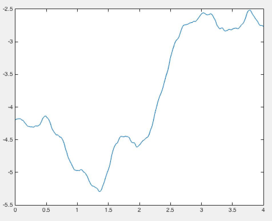
Fitting an FOU to the 2 hours of data with GPML yields time constants and around mins and secs, though one can not say from the data analysis which is which (that is an interesting challenge). It is again awkward that the data is not available at more frequent intervals than 1 second, as the determined time constant 1.87 sec is close to this limit. A more thorough treatment would evaluate the posterior uncertainty in the parameter fits and attempt to resolve the discrepancies between the previously estimated OU time constant of 30 mins and the current one of 11.1 mins, and between the eyeball estimate Hz from Fig 6 of where the slope changes, giving a time constant of around 4 sec, and the current one of 1.87 sec.
Over long timescales, deviations from Gaussianity have been established [47]. Nevertheless, I believe this does not invalidate Gaussian modelling for short times.
To take this project further, we need next to tackle how a typical two-node system behaves. This would be the simplest system that could show an inter-area oscillation. It needs data for the phase difference between the two nodes and their frequencies, and it needs the Kalman filter coding up for at least five dimensions (2 frequencies, 1 phase difference, 2 power imbalances).
8 Discussion
I have presented a method to detect oscillations in systems with many components. It is promising because it can integrate data from many locations simultaneously to enhance the sensitivity of detection of modes of oscillation, and it can run in real-time with constant computation time per observation.
[19] consider the problem of calculating modes and mode shapes from phasor measurement units (PMU) in an AC electrical network to have been solved. They cite [40, 61, 33, 7]. I am not so convinced. I think it would be good to try the method of this paper on that problem.
Detection of modes of oscillation is important in many other contexts. One example is to detect soft (i.e. lightly damped) modes for civil engineering structures such as buildings and bridges, e.g. Ch.13 of [25]. Another is the identification of modes of oscillation in the sun (helioseismology), which enables to deduce its temperature and rotation profiles [27]. A third is the analysis of gene expression data, e.g. [39]. A fourth is the analysis of business cycles, e.g. Ch.4 of [46], which have been seen for a long time but are still not understood.
Detection of oscillations is a very old subject, so we next give a brief review of traditional methods.
A standard approach to detecting oscillations is to identify peaks in the Fourier spectrum [25] or variants [11]. For example, the response of the second-order system
| (71) |
to noise with power spectrum has power spectrum
| (72) |
as a function of frequency . So if the noise is white ( is constant), then the inverse quality factor is precisely the fullwidth at half maximum for the power spectrum of the velocity (its maximum is at , known as the resonant frequency), and the damping ratio is the halfwidth at half maximum. For slowly varying on the scale of , the results remain good approximations. This was given a sound grounding in Bayesian analysis (see [22] for a survey and [10] for a pedagogical presentation), but still suffers from issues like dealing with trends, choosing windowing functions, missing data, failure to cater for slowly shifting phase, and poor theoretical justification for taking more than the largest peak if one wants to infer more than one mode of oscillation.
Wavelet transforms are popular for resolving signals in both time and frequency (up to the limits of the uncertainty principle), but I am not aware whether they can give an estimate of damping rate.
Another approach is to study the effect of an impulse (the Prony method and variants like MUSIC and ESPRIT, e.g. [36]), but many real-world systems may not be subjectable to impulses. For a review of these and some other methods (e.g. Hilbert transform), see [62].55 5 As yet another method, I learnt back in the mid-1980s that a good way to determine the eigenvalues of an asymptotically stable system from the response to an impulse is to Laplace transform the response numerically and then fit a Padé approximation and read off its poles. One defect of the approach is that the forcing might not be Gaussian. For example, even a Poisson process with independent Gaussian amplitude is not Gaussian. Indeed, a consequence of the Gaussian assumption is that the covariance of the response is time-symmetric, whereas this may not be true for real systems. As already mentioned, evidence for Gaussian distribution of electrical load is given in Fig.14 of [57], but they do not report on time-correlation. Load variations are likely to be independent, however, which would make them Gaussian and white. On the other hand, wind power is unlikely to be delta-correlated. There is considerable research on the statistics of wind power, e.g. [14, 54, 58].
Another defect of the approach is that it does not allow for nonlinearity. Nevertheless, for small fluctuations around an equilibrium, linearising is a good approach. It will fail to give a good approximation, however, if the eigenvalues of any mode approach or cross the imaginary axis. A big question with power flow oscillations, gene expression and business cycles is whether there is a limit cycle of some underlying deterministic dynamics, or just lightly damped oscillations around an equilibrium forced by noise. Figure 1 suggests to me that there was a Hopf bifurcation, but the common wisdom in the power system community is that it was just a large kick that set off a lightly damped mode of oscillation. For gene expression this has been addressed by [15]. For business cycles, most economists decided long ago that they are just a near unit root process (meaning lightly damped oscillations forced by shocks) [46], though Grandmont proposed deterministic models with a variety of forms of dynamics [21]. [48] fitted a VAR model, but with perhaps too many free parameters. Our approach would restrict to a small number of modes.
An interesting issue is that if the noise is considered to be the result of filtering white noise then our method also finds the modes of the filter. Without further information about the structure of the system or direct observations of the forcing process, we see no way of distinguishing between modes of the filter and modes of the system from observations of just the system. An example of this was given in Section 7.
To detect periodic components, my brother David [30] proposed the family of stationary covariance functions of the form
| (73) |
for which samples are exactly periodic with period . A slight modification was used in [28] to remove the effect of its non-zero mean, namely
| (74) |
where is a modified Bessel function of the first kind. It has the limiting form
| (75) |
as , called the Cos kernel, which has the property that it forces anti-periodicity with anti-period : . Although these have found valuable uses, and can be made less rigid by multiplication by a decaying kernel such as (which with the Cos kernel produces OUosc), it seems to me highly preferable to start from the point of view of a linear system forced by noise.
I conclude with a suggested improved approach to nuclear magnetic resonance imaging. The present standard approach is to apply an electromagnetic pulse that simultaneously excites all the single-quantum NMR transitions. The resulting time-domain signal is Fourier transformed to reveal NMR absorption intensity against frequency. I suggest instead to apply electromagnetic noise and from the resulting response to infer the frequencies and damping rates by the Gaussian processes of this paper.
Acknowledgements
I am grateful to Ben Marshall of National Grid for proposing the problem of detecting inter-area oscillations in Jan 2015, and to him and his colleague Phillip Ashton for helpful discussions on the topic and pointers to the literature; to MSc student Tajhame Francis for initial investigations by spectral analysis; to my brother David for telling me to “Use a Gaussian process"; to PhD student Marcos Tello Fraile and postdoc Lisa Flatley for trying to follow my suggestions; to Hannes Nickisch and Colm Connaughton for helping me implement my resulting solutions in GPML; to Carl Rasmussen and Hannes Nickisch for having created GPML; to Zoubin Ghahramani for answering some questions about GPs; to Igor Mezic and Yoshihiko Susuki for discussions on modelling AC networks; to undergraduate summer project student John Prater for coding up the underdamped linear Langevin covariance for GPML; and to Chris Williams, Darren Wilkinson and especially Janusz Bialek for useful comments and questions. The beginning of the work was supported by National Grid under Network Innovation Allowance award NIA_NGET0161. The later parts were supported by the Alan Turing Institute under award TU/B/000101.
References
References
- [1] Abrahamsen P, A review of Gaussian random fields and correlation functions (2nd ed, 1997)
- [2] Adler RJ, The geometry of random fields (Wiley, 1981).
- [3] Alston C, Kuhnert P, Low Choy S, McVinish R, Mengersen K, Bayesian model comparison: review and discussion, in: Internat Stat Institute 55th session (2005).
- [4] Alvarez M, Luengo D, Lawrence ND, Latent force models, in: Proc 12th AISTATS (2009)
- [5] Ammar GS, Gragg WB, The generalised Schur algorithm for the superfast solution of Toeplitz systems, in Rational approximation and its applications in mathematics and physics, eds Gilewicz J, Pindor M, Siemaszko W, Lect Notes Math 1237 (Springer, 1987) 315–330.
- [6] Andersson G, Power system analysis (ETH lecture notes, 2012)
- [7] Barocio E, Pal BC, Thornhill NF, Messina AR, A dynamic mode decomposition framework for global power system oscillation analysis, IEEE Trans Power Sys 30:6 (2015) 2902–12.
- [8] Bhatia R, Rosenthal P, How and why to solve the operator equation , Bull Lond Math Soc 29 (1997) 1–21.
- [9] Boyle P, Frean M, Dependent Gaussian Processes, Adv Neural Info Processing Sys (2005)
- [10] Bretthorst GL, Bayesian spectrum analysis and parameter estimation, Lect Note Stats 48 (Springer, 1988).
- [11] Brincker R, Zhang L, Andersen P, Output-only modal analysis by frequency domain decomposition, Proc ISMA25 (2000), vol.2, 7pp.
- [12] Bui TD, Nguyen CV, Turner RE, Streaming sparse Gaussian process approximations, arXiv: 1705.07131v2 (2017)
- [13] Caines PE, Linear stochastic systems (Wiley, 1988).
- [14] D’Amico G, Petroni F, Prattico F, Wind speed prediction for wind farm applications by extreme value theory and copulas, J Wind Eng Ind Aerodyn 145 (2015) 229–36.
- [15] Durrande N, Hensman J, Rattray M, Lawrence ND, Detecting periodicities with Gaussian processes, arXiv:1303.7090v2 (2016)
- [16] Gallivan K, Thirumalai S, Dooren P van, On solving block Toeplitz systems using a block Shur algorithm, Parallel Processing 1994 (IEEE conf) vol.3, 274–281.
- [17] Gardiner CW, Stochastic Methods (Springer, 1985, 2009)
- [18] Gibbard MJ, Pourbeik P, Vowles DJ, Small-signal stability, control and dynamics performance of power systems (Univ Adelaide Press, 2015)
- [19] Gorbunov A, Dymarsky A, Bialek J, Estimation of parameters of a dynamic generator model from modal PMU measurements, IEEE Trans Power Sys, to appear
- [20] Grainger JJ, Stevenson WD, Power system analysis (McGraw-Hill, 1994).
- [21] Grandmont J-M, On endogeneous competitive business cycles, Econometrica 53 (1985) 995–1045.
- [22] Gregory PC, A Bayesian revolution in spectral analysis, in: Bayesian inference and maximum entropy methods in Science and Engineering, ed Mohammad-Djafari A, Am Inst Phys Conf Proc 568 (2001) 557–68.
- [23] Han S, Rong N, Sun T, Zhang J, An approach for estimating mode shape for participation of inter-area oscillation mode, IEEE Internat Symp on Circuits & Systems (ISCAS), (2013) 2968–71.
- [24] Hartikainen J, Särkkä S, Kalman filtering and smoothing solutions to temporal Gaussian process regression models, Proc IEEE Internat Workshop on Machine Learning for Signal Processing 2010
- [25] He J, Fu Z-F, Modal analysis (Butterworth-Heinemann, 2001).
- [26] Janssens N, Kamagate A, Interarea oscillations in power systems, IFAC Power Plants and Power System Conotrol (Brussels, 2000), 217–226.
- [27] Kosovichev AG, Solar oscillations, in Stellar Pulsation, AIP Conf Proc 1170 (2009) 547–559.
- [28] Lloyd JR, Duvenaud D, Grosse R, Tenenbaum JB, Ghahramani Z, Automatic construction and natural-language description of nonparametric regression models, arXiv:1402.4304 (2014)
- [29] Machowski J, Bialek JW, Bumby JR, Power system dynamics (second ed, Wiley, 2008)
- [30] MacKay DJC, Introduction to Gaussian Processes, NATO ASI series F Comp Sys Sci 168 (1998) 133–66.
- M [2] MacKay DJC, Information theory, Inference, and Learning algorithms (Cambridge Univ Press, 2003).
- [32] MacKay RS, Phillips NE, A natural 4-parameter family of covariance functions for stationary Gaussian processes, http://arxiv.org/abs/1810.07738
- [33] Messina A, Vittal V, Extraction of dynamic patterns from wide-area measurements using empirical orthogonal functions, IEEE Trans Power Sys 22:2 (2007) 682–92
- [34] http://www2.nationalgrid.com/Enhanced-Frequency-Response.aspx
- [35] Papoulis A, Probability random variables and stochastic processes (1991)
- [36] Papy JM, Latauwer L de, Huffel S van, Exponential data fitting using multilinear algebra: The single-channel and multi-channel case, Numer Lin Alg Appl 12 (2005) 809-26.
- [37] Park H, Elden L, Schur-type methods for solving least squares problems with Toeplitz structure, SIAM J Sci Comput 22 (2000) 406–430.
- [38] Paserba J (convenor), Analysis and control of power system oscillations (CIGRE, 1996) brochure 111
- [39] Phillips NE, Manning C, Papalopulu N, Rattray M, Identifying stochastic oscillations in single-cell live imaging time series using Gaussian processes, arXiv: 1608.06476v2 (2016)
- [40] Pierre JW, Trudnowski DJ, Donnelly MK, Initial results in electromechanical mode identification from ambient data, IEEE Trans Power Sys 12:3 (1997) 1245–51.
- [41] Rasmussen CE, Williams CKI, Gaussian processes for machine learning (MIT press, 2006).
- [42] Reece S, Roberts S, An introduction to Gaussian processes for the Kalman filter expert, in: Information Fusion 2010 (IEEE), doi: 10.1109/ICIF.2010.5711863
- [43] Reece S, Ghosh S, Rogers A, Jennings N, Roberts S, Efficient state-space inference of periodic latent force models, arXiv 1310.6319v2 (2014)
- [44] Roberts S, Osborne M, Ebden M, Reece S, Gibson N, Aigrain S, Gaussian processes for timeseries modelling, Phil Trans Roy Soc Lond A 371 (2013) 20110550.
- [45] Roger G, Power system oscillations (Kluwer, 2000).
- [46] Romer D, Advanced Macroeconomics (McGraw-Hill, 2001)
- [47] Schäfer B, Beck C, Aihara K, Witthart D, Timme D, Non-Gaussian power grid frequency fluctuations characterised by Lévy-stable laws and superstatistics, Nature Energy 3 (2018) 119–26.
- [48] Sims CA, Macroeconomics and reality, Econometrica 48 (1980) 1–48.
- [49] Stewart M, Cholesky factorization of semidefinite Toeplitz matrices, Lin Alg Applns 254 (1997) 497–525.
- [50] Susuki Y, Mezic I, Nonlinear Koopman modes and a precursor to power system swing instabilities, IEEE Trans Power Sys 27 (2012) 1182–91.
- [51] Susuki Y, Mezic I, Hikihara T, Coherent swing instability of interconnected power grids and a mechanism of cascading failure, in: Control and optimisation methods for electric smart grids, eds Chakraborty A, Ilic MD (Springer, 2012) 185–202.
- [52] Tobar F, Bui TD, Turner RE, Learning stationary time series using Gaussian Processes with nonparametric kernels, Adv Neural Info Processing Sys 27 (MIT Press, 2015)…
- [53] Trip S, Bürger M, Persis C De, An internal model approach to (optimal) frequency regulation in power grids with time-varying voltages, arXiv: 1403.7019v3 (2015)
- [54] Troffaes MCM, Williams E, Dent CJ, Data analysis and robust modelling of the impact of renewable generation on long term security of supply and demand, in: 2015 IEEE Power and Energy Society General Meeting, 1–5.
- [55] Trudnowski DJ, Estimating electromechanical mode shape from synchrophasor measurements, IEEE Trans Power Sys 23 (2008) 1188–95.
- [56] Turunen J, Renner H, Hung WW, Carter AM, Ashton PM, Haarla LC, Simulated and measured inter-area mode shapes and frequencies in the electrical power system of Great Britain, in IET International Conference on Resilience of Transmission and Distribution Networks (RTDN2015) (IET, 2015) 136–141.
- [57] Turunen J, Thambirajah J, Larsson M, Pal BC, Thornhill NF, Haarla LC, Hung WW, Carter AM, Rauhala T, Comparison of three electromechanical oscillation damping estimation methods, IEEE Trans Power Sys 26 (2011) 2398–2407
- [58] Wadman WS, Bloemhof G, Crommelin D, Frank J, Probabilistic power flow simulation allowing temporary current overloading, Proc PMAPS 2012 (2012) 494–9.
- [59] Wang X, Bialek JW, Turitsyn K, PMU-Based Estimation of Dynamic State Jacobian Matrix and Dynamic System State Matrix in Ambient Conditions, IEEE Trans Power Sys 33:1 (2018) 681–690.
- [60] West M, Harrison PJ, Bayesian forecasting and dynamic models (Springer, 1989).
- [61] Zhou N, Trudnowski DJ, Pierre JW, Mittelstadt, Electromechanical mode online estimation using regularised robust RLS methods, IEEE Trans Power Sys 23:4 (2008) 1670–80.
- [62] Zielinski TP, Duda K, Frequency and damping estimation methods - an overview, Metrol Meas Syst 18 (2011) 505–28.