跳到论文正文
W Papers独立论文阅读器 arXiv:1909.10206 论文正文 计算阅读时间 · 0%
引用这篇论文根据当前论文元数据生成,正式投稿前建议核对。


License: arXiv.org perpetual non-exclusive license
arXiv:1909.10206v2 [cs.IT] 02 Jan 2020

Cross Z-Complementary Pairs (CZCPs) for Optimal Training in Spatial Modulation Over Frequency Selective Channels

Zilong Liu    Ping Yang    Yong Liang Guan    Pei Xiao Thanks: Zilong Liu is with School of Computer Science and Electronic Engineering, University of Essex, United Kingdom (e-mail: zilong.liu@essex.ac.uk). Ping Yang is with National Key Laboratory on Communications, University of Electronic Science and Technology of China, Chengdu, China (e-mail: yang.ping@uestc.edu.cn). Pei Xiao is with Institute for Communication Systems, 5G Innovation Centre, University of Surrey, United Kingdom (e-mail: p.xiao@surrey.ac.uk). Yong Liang Guan is with the School of Electrical and Electronic Engineering, Nanyang Technological University, Singapore (E-mail: eylguan@ntu.edu.sg).
Abstract

The contributions of this paper are twofold: Firstly, we introduce a novel class of sequence pairs, called “cross Z-complementary pairs (CZCPs)”, each displaying zero-correlation zone (ZCZ) properties for both their aperiodic autocorrelation sums and crosscorrelation sums. Systematic constructions of perfect CZCPs based on selected Golay complementary pairs (GCPs) are presented. Secondly, we point out that CZCPs can be utilized as a key component in designing training sequences for broadband spatial modulation (SM) systems. We show that our proposed SM training sequences derived from CZCPs lead to optimal channel estimation performance over frequency-selective channels.

Index Terms: 
Golay complementary pairs (GCPs), channel estimation, training sequence design, spatial modulation, frequency-selective channels.

I Introduction

This paper investigates a novel class of sequence pairs called “cross Z-complementary pairs (CZCPs)” and their applications for training sequence design in broadband spatial modulation (SM) systems. In what follows, we review the state-of-the-art on pairs of sequences and SM, then introduce our contributions in this work.

I-A Pairs of Sequences

“Pairs of sequences” has been an attractive research topic since the invention of complementary pairs proposed by Marcel J. E. Golay in 1951 [1]. It was found by Golay that infrared multislit spectrometry, a device which isolates a desired radiation with a fixed single wavelength from background radiation (with many different wavelengths), can be designed with the aid of a special class of pairs of sequences, which is widely known as Golay complementary pair (GCP).

Let 𝐚\mathbf{a} and 𝐛\mathbf{b} be two sequences of identical length. Denote by ρ​(𝐚,𝐛)​(τ)\rho(\mathbf{a},\mathbf{b})(\tau) their aperiodic crosscorrelation (ACC) at time-shift τ\tau (formal definition of ACC will be given in Section II). For simplicity, when 𝐚=𝐛\mathbf{a}=\mathbf{b}, ρ​(𝐚,𝐛)​(τ)\rho(\mathbf{a},\mathbf{b})(\tau) will be written as ρ​(𝐚)​(τ)\rho(\mathbf{a})(\tau). By definition, (𝐚,𝐛)(\mathbf{a},\mathbf{b}) is said to be a GCP if ρ⁡(𝐚)​(τ)+ρ⁡(𝐛)​(τ)=0\rho(\mathbf{a})(\tau)+\rho(\mathbf{b})(\tau)=0 for all τ≠0\tau\neq 0. In principle, sequences in a GCP work in a cooperative way so that their aperiodic autocorrelations (AAC) sums vanish for all the non-zero time-shifts [2].

For more than 60 years, huge amount of research effort has been made on the constructions of GCPs. Recursive algorithms proposed by Budišin in 1990s for polyphase and multi-level GCPs can be found in [3, 4]. Theory on para-unitary (PU) matrices has recently been applied for more efficient GCP synthesis [5, 6, 7, 8]. In 1999, Davis and Jedwab developed a direct construction of polyphase GCPs through generalized Boolean functions [9]. Their construction was extended to GCPs over QAM constellations using weighted sum of several QPSK GCPs [10, 11]. Existing known binary GCPs have even lengths of the form 2α​10β​26γ2^{\alpha}10^{\beta}26^{\gamma} only, where α,β,γ\alpha,\beta,\gamma are non-negative integers satisfying α+β+γ≥1\alpha+\beta+\gamma\geq 1 [12], [13]. For sequence pairs with odd lengths, the best known alternative to GCPs is optimal odd-length binary Z-complementary pairs (OB-ZCPs) [14] each displaying the largest zero-correlation zone (ZCZ) width [15] and minimum AAC sums outside the ZCZ.

GCPs and their extension, called “complementary codes (CC)” [16, 17], have found applications far beyond their initial usage in the design of multislit spectrometry. A few selected applications in wireless communications include: optimal channel estimation in multiple-input multiple-output (MIMO) frequency-selective channels [18, 19], Doppler-resilient waveform design [20, 21], interference-free multi-carrier code-division multiple-access (MC-CDMA) communications [22, 23, 24], and power control in MC communications [9, 10, 11, 25, 26, 27].

It should be noted that each GCP, ZCP or CC, is defined by their AAC sums only. Within each GCP, ZCP or CC, it is assumed that separate non-interfering channels are used for the transmission of the constituent sequences. Crosscorrelations between constituent sequences within each GCP, ZCP or CC, have not been considered.

I-B Spatial Modulation (SM)

MIMO is a revolutionary communication paradigm which can achieve significant increase in spectral efficiency and enhanced robustness against fading through exploitation of spatial diversity [28, 29, 30, 31, 32, 33, 34]. SM is a special class of MIMO techniques which trades multiplexing gain with complexity and performance [35, 36, 37, 38, 39]. Unlike conventional MIMO, an SM system is equipped with multiple transmit antenna (TA) elements but only a single radio-frequency (RF) chain. During each time-slot, an SM symbol can be divided into two parts: one (called “spatial symbol”) is responsible for the selection and then activation of a TA element, the other (called “constellation symbol”) is selected from a conventional PSK/QAM constellation and transmitted from the active TA element. Such unique transmission principle of SM allows it to have at least the following advantages over conventional MIMO:

  1. 1.

    Zero inter-channel interference (ICI) over flat fading channels and thus improved average bit error probability;

  2. 2.

    Lower hardware complexity in the transmitter (due to its single RF chain) and lower detection complexity at the receiver (due to zero ICI);

  3. 3.

    Lower energy consumption which makes SM a promising candidate for large-scale antenna systems [40].

Early literature on SM mostly assume that channel state information (CSI) is perfectly known at the receiver [41, 42]. Effects of channel estimation errors to the performance of SM systems, limited to flat-fading channels, have been studied in [43, 44, 45, 46]. Up to date, however, little has been understood on channel estimation of SM in frequency-selective channels. Along this research direction, two fundamental research problems arise and will be addressed in this work: 1) What is the lower bound on the channel estimation mean-squares-error (MSE)? 2) How to design efficient channel training scheme to meet this lower bound with equality?

Note that the “one-RF-chain” principle of SM prevents the transmitter from using simultaneous pilot transmission over all the TAs. Consequently, it implies that dense training sequences proposed in [48, 49, 50] for traditional MIMO are unapplicable in SM systems. Although an identity training matrix has been employed for joint channel estimation and data detection in SM systems [45], extension to frequency-selective channels is not straightforward. A naive scheme is to extend a perfect sequence (having zero autocorrelation sidelobes) with cyclic-prefix (CP)11 1 whose duration should be not smaller than the largest multipath delay. and then send the extended sequence in turn over multiple TAs. But this training scheme would be inefficient in highly dispersive channels.

I-C Contributions of This Paper

The main contributions of this work are summarized as follows.

  1. 1.

    We introduce a novel class of sequence pairs, called CZCPs, each displaying certain ZCZ properties for both their AAC sums and ACC sums. Specifically, a pair of sequences, say (𝐚,𝐛)(\mathbf{a},\mathbf{b}), is called a CZCP if ρ​(𝐚)​(τ)+ρ​(𝐛)​(τ)\rho(\mathbf{a})(\tau)+\rho(\mathbf{b})(\tau) and ρ⁡(𝐚,𝐛)​(τ)+ρ⁡(𝐛,𝐚)​(τ)\rho(\mathbf{a},\mathbf{b})(\tau)+\rho(\mathbf{b},\mathbf{a})(\tau) take zero values for certain time-shifts τ\tau. The most distinctive feature of CZCPs (compared to conventional sequence pairs) is that the two constituent sequences in a CZCP may interfere with each other during the transmission. Therefore, careful design should be carried out to force their cross-interference to zero in a certain τ\tau region. We investigate the structural properties of CZCPs and show that a subset of GCPs are perfect CZCPs.

  2. 2.

    We present a generic training framework for SM training over frequency selective channels. Under this framework, we derive the lower bound on channel estimation MSE using least square (LS) estimator and conditions to meet this lower bound with equality. Then, we show that CZCPs play an instrumental role in the design of optimal SM training sequences (which are equivalent to certain sparse matrices). Numerical simulations indicate that the proposed SM training sequences lead to minimum channel estimation MSE w.r.t. the aforementioned lower bound.

I-D Organization of This Paper

This paper is organized as follows. Section II introduces some notations and GCPs, followed by a sketch of the basic principle of SM. In Section III, we formally define CZCPs, give their structural properties, and then present perfect CZCPs obtained from computer search and systematic constructions. Section IV starts from a generic framework on the training design of SM, under which a lower bound on the channel estimation MSE is derived. Then, CZCPs are applied to design sparse training matrices for optimal channel estimation performance (w.r.t. the derived lower bound) in SM-MIMO frequency selective channels. In the end of Section IV, we evaluate the proposed SM training scheme using numerical simulations. Finally, Section V concludes this paper.

II PRELIMINARIES

II-A Notations

The following notations will be used throughout this paper.

  • −-

    𝐗T\mathbf{X}^{\text{T}} and 𝐗H\mathbf{X}^{\text{H}} denote the transpose and the Hermitian transpose of matrix 𝐗\mathbf{X}, respectively;

  • −-

    ‖𝐗‖=∑m=1M∑n=1N|xm,n|2\|\mathbf{X}\|=\sqrt{\sum_{m=1}^{M}\sum_{n=1}^{N}|x_{m,n}|^{2}} denotes the Frobenius norm of matrix 𝐗=[xm,n]m,n=1M,N\mathbf{X}=[x_{m,n}]_{m,n=1}^{M,N};

  • −-

    <𝐱,𝐲><\mathbf{x},\mathbf{y}> denotes the inner-product between two complex-valued sequences 𝐱=[x0,x1,⋯,xN−1]T\mathbf{x}=[x_{0},x_{1},\cdots,x_{N-1}]^{\text{T}} and 𝐲=[y0,y1,⋯,yN−1]T\mathbf{y}=[y_{0},y_{1},\cdots,y_{N-1}]^{\text{T}}, i.e., <𝐱,𝐲>=∑i=0N−1xi​yi∗<\mathbf{x},\mathbf{y}>=\sum\limits_{i=0}^{N-1}x_{i}y^{*}_{i}, where NN is the sequence length of 𝐱\mathbf{x} (and 𝐲\mathbf{y});

  • −-

    Tτ​(𝐱)T^{\tau}({\mathbf{x}}) denotes the right-cyclic-shift of 𝐱=[x0,x1,⋯,xN−1]T\mathbf{x}=[x_{0},x_{1},\cdots,x_{N-1}]^{\text{T}} for τ\tau (nonnegative integer) positions, i.e.,

    Tτ​(𝐱)=[xN−τ,⋯,xN−1⏟the last ​τ​elements of​𝐱,x0,x1,⋯,xN−τ−1]T.T^{\tau}({\mathbf{x}})=[\underbrace{x_{N-\tau},\cdots,x_{N-1}}_{\text{the last~}\tau~\text{elements of}~\mathbf{x}},x_{0},x_{1},\cdots,x_{N-\tau-1}]^{\text{T}}.

    Similarly,

    T−τ​(𝐱)=[xτ,xτ+1,⋯,xN−1,x0,x1,⋯,xτ−1⏟the first ​τ​elements of ​𝐱]T.T^{-\tau}({\mathbf{x}})=[x_{\tau},x_{\tau+1},\cdots,x_{N-1},\underbrace{x_{0},x_{1},\cdots,x_{\tau-1}}_{\text{the first~}\tau~\text{elements of~}\mathbf{x}}]^{\text{T}}.
  • −-

    𝐱¯\underline{\mathbf{x}} denotes the reversal of vector 𝐱=[x0,x1,⋯,xN−1]T\mathbf{x}=[x_{0},x_{1},\cdots,x_{N-1}]^{\text{T}}, i.e., 𝐱¯=[xN−1,xN−2,⋯,x0]T\underline{\mathbf{x}}=[x_{N-1},x_{N-2},\cdots,x_{0}]^{\text{T}};

  • −-

    Diag​[𝐱]\text{Diag}[\mathbf{x}] denotes a diagonal matrix with the diagonal vector of 𝐱\mathbf{x} and zero for all off-diagonal entries;

  • −-

    𝟏m×n\mathbf{1}_{m\times n} and 𝟎m×n\mathbf{0}_{m\times n} denote an all-1 matrix and an all-0 matrix, respectively, both having matrix order of m×nm\times n;

  • −-

    𝐈N\mathbf{I}_{N} denotes the identity matrix of order NN;

  • −-

    ⊗\otimes denotes the Kronecker product operator;

  • −-

    ⌊j⌋J\lfloor j\rfloor_{J} denotes the modulo JJ operation of integer jj, e.g., ⌊4⌋4=0,⌊5⌋4=1\lfloor 4\rfloor_{4}=0,\lfloor 5\rfloor_{4}=1;

  • −-

    Denote ωq=exp⁡(2​π​−1q)\omega_{q}=\exp\left(\frac{2\pi\sqrt{-1}}{q}\right) (integer qq);

  • −-

    ℤq\mathbb{Z}_{q} denotes the set of integers modulo qq, i.e., ℤq={0,1,⋯,q−1}\mathbb{Z}_{q}=\{0,1,\cdots,q-1\} (qq integer);

  • −-

    𝒜q={ωq0,ωq1,⋯,ωqq−1}\mathcal{A}_{q}=\{\omega^{0}_{q},\omega^{1}_{q},\cdots,\omega^{q-1}_{q}\} denotes the set over qq complex roots of unity.

  • −-

    𝔼⁡(x)\mathbb{E}(x) denotes the mean of random variable xx;

  • −-

    Tr​(𝐗)\text{Tr}(\mathbf{X}) denotes the trace of square matrix 𝐗\mathbf{X}.

For two length-NN complex-valued sequences

𝐚=[a0,a1,⋯,aN−1]T,𝐛=[b0,b1,⋯,bN−1]T,\mathbf{a}=[a_{0},a_{1},\cdots,a_{N-1}]^{\text{T}},~~\mathbf{b}=[b_{0},b_{1},\cdots,b_{N-1}]^{\text{T}},

denote by ρ​(𝐚,𝐛)​(τ)\rho({\mathbf{a}},{\mathbf{b}})\left(\tau\right) the ACC between 𝐚\mathbf{a} and 𝐛\mathbf{b}, i.e.,

ρ⁡(𝐚,𝐛)​(τ)={∑n=0N−τ−1an​bn+τ∗,0≤τ≤N−1,∑n=0N+τ−1an−τ​bn∗,−(N−1)≤τ≤−1,0,|τ|≥N.\rho({\mathbf{a}},{\mathbf{b}})\left(\tau\right)=\begin{cases}{\sum\limits_{n=0}^{N-\tau-1}{a_{n}{b^{*}_{n+\tau}}}},&~0\leq\tau\leq N-1,\\ {\sum\limits_{n=0}^{N+\tau-1}{a_{n-\tau}{b^{*}_{n}}}},&~-(N-1)\leq\tau\leq-1,\\ 0,&~|\tau|\geq N.\end{cases} (1)

Also, denote by ϕ​(𝐚,𝐛)​(τ)\phi({{\mathbf{a}},{\mathbf{b}}})\left(\tau\right) the periodic cross-correlation (PCC) between 𝐚\mathbf{a} and 𝐛\mathbf{b}, i.e.,

ϕ(𝐚,𝐛)(τ)=∑n=0N−1anb⌊n+τ⌋N∗=⟨𝐚,T−τ(𝐛)⟩.\phi({{\mathbf{a}},{\mathbf{b}}})\left(\tau\right)=\sum\limits_{n=0}^{N-1}{a_{n}}{b^{*}_{\lfloor n+\tau\rfloor_{N}}}=\Bigl<\mathbf{a},T^{-\tau}(\mathbf{b})\Bigl>. (2)

Clearly, ρ⁡(𝐚,𝐛)​(τ)=ρ∗​(𝐚,𝐛)​(−τ)\rho({{\mathbf{a}},{\mathbf{b}}})\left(\tau\right)=\rho^{*}({{\mathbf{a}},{\mathbf{b}}})\left(-\tau\right) and

ϕ⁡(𝐚,𝐛)​(τ)=ρ⁡(𝐚,𝐛)​(τ)+ρ∗​(𝐛,𝐚)​(N−τ).\phi({{\mathbf{a}},{\mathbf{b}}})\left(\tau\right)=\rho({{\mathbf{a}},{\mathbf{b}}})\left(\tau\right)+\rho^{*}({{\mathbf{b}},{\mathbf{a}}})\left(N-\tau\right). (3)

In particular, when 𝐚=𝐛\mathbf{a}=\mathbf{b}, ρ​(𝐚,𝐚)​(τ)\rho({{\mathbf{a}},{\mathbf{a}}})(\tau) will be sometimes written as ρ​(𝐚)​(τ)\rho({{\mathbf{a}}})(\tau) and called the AAC of 𝐚\mathbf{a} at time-shift τ\tau. Similarly, ϕ​(𝐚,𝐚)​(τ)\phi({{\mathbf{a}},{\mathbf{a}}})(\tau) will be sometimes written as ϕ​(𝐚)​(τ)\phi({{\mathbf{a}}})(\tau) and called the periodic auto-correlation (PAC) of 𝐚\mathbf{a}.

II-B Introduction to Golay Complementary Pair (GCP)

Next, we give a brief introduction to GCPs. We will show in Section III that a subset of GCPs are perfect CZCPs.

Definition 1

(𝐚,𝐛)(\mathbf{a},\mathbf{b}) is called a GCP if their AAC sum equals zero for any non-zero time-shift τ\tau, i.e.,

ρ⁡(𝐚)​(τ)+ρ⁡(𝐛)​(τ)=0,∀τ≠0.\rho({{\mathbf{a}})\left(\tau\right)+\rho({\mathbf{b}}})\left(\tau\right)=0,~\forall~\tau\neq 0. (4)

Furthermore, two GCPs (𝐚,𝐛)(\mathbf{a},\mathbf{b}) and (𝐜,𝐝)(\mathbf{c},\mathbf{d}) are said to be mutually orthogonal if they have zero ACC sums for all time-shifts, i.e.,

ρ⁡(𝐚,𝐜)​(τ)+ρ⁡(𝐛,𝐝)​(τ)=0,\rho(\mathbf{a},\mathbf{c})\left(\tau\right)+\rho(\mathbf{b},\mathbf{d})\left(\tau\right)=0, (5)

holds for any arbitrary τ\tau. As a matter of fact, (𝐛∗¯,−𝐚∗¯)(\underline{\mathbf{b}^{*}},-\underline{\mathbf{a}^{*}}) is a GCP which is mutually orthogonal to (𝐚,𝐛)(\mathbf{a},\mathbf{b}) [12], where 𝐛¯\underline{\mathbf{b}} denotes the reversal of 𝐛\mathbf{b}.

Definition 2

For 𝐱=[x1,x2,…,xμ]∈ℤ2μ\mathbf{x}=[x_{1},x_{2},\ldots,x_{\mu}]\in\mathbb{Z}_{2}^{\mu}, a generalized Boolean function (GBF) g⁡(𝐱)g(\mathbf{x}) is defined as a mapping g:{0,1}μ→ℤqg:\{0,1\}^{\mu}\rightarrow\mathbb{Z}_{q}. Each variable xix_{i} (i∈{1,2,…,μ}i\in\{1,2,\ldots,\mu\}) in 𝐱\mathbf{x} may be regarded as a GBF (see Example 1). Let [κ1,κ2,…,κμ][\kappa_{1},\kappa_{2},\ldots,\kappa_{\mu}] be the binary representation of the (non-negative) integer κ=∑i=1μκi​2i−1\kappa=\sum_{i=1}^{\mu}\kappa_{i}2^{i-1}, with κμ\kappa_{\mu} denoting the most significant bit and 0≤κ≤2μ−10\leq\kappa\leq 2^{\mu}-1. Given g⁡(𝐱)g(\mathbf{x}), define gκ≜g⁡(κ1,κ2,…,κμ)g_{\kappa}\triangleq g(\kappa_{1},\kappa_{2},\ldots,\kappa_{\mu}) and its associated sequence

𝐠≜[g0,g1,…,g2μ−1].\mathbf{{g}}\triangleq\Bigl[g_{0},g_{1},\ldots,g_{2^{\mu}-1}\Bigl]. (6)

Furthermore, we define a complex-valued sequence associated to GBF gg as follows.

φq(𝐠)≜[ωqg0,ωqg1,…,ωqg2μ−1].\varphi_{q}(\mathbf{g})\triangleq\Bigl[\omega_{q}^{g_{0}},\omega_{q}^{g_{1}},\ldots,\omega_{q}^{g_{2^{\mu}-1}}\Bigl]. (7)

It is stressed that each realization of gκg_{\kappa} is obtained by setting x1=κ1,x2=κ2,…,xμ=κμx_{1}=\kappa_{1},x_{2}=\kappa_{2},\ldots,x_{\mu}=\kappa_{\mu} into the GBF gg, for a specific κ\kappa. Hence, if g=xtg=x_{t}, where 1≤t≤μ1\leq t\leq\mu, the associated sequence 𝐠\mathbf{g} is the vector formed by gκ=κtg_{\kappa}=\kappa_{t}, when κ\kappa ranges from 00 to 2μ−12^{\mu}-1. In this case, we denote the corresponding 𝐠\mathbf{g} by 𝐱t\mathbf{x}_{t}, i.e., 𝐠=𝐱t\mathbf{g}=\mathbf{x}_{t}. Similarly, if g=xt1​xt2g=x_{t_{1}}x_{t_{2}} (t1≠t2t_{1}\neq t_{2}), we write 𝐠=𝐱t1​𝐱t2\mathbf{g}=\mathbf{x}_{t_{1}}\mathbf{x}_{t_{2}}, a vector obtained by element-wise multiplication of 𝐱t1\mathbf{x}_{t_{1}} and 𝐱t2\mathbf{x}_{t_{2}}. We need the following definition which will be used in Section III to identify a subset of GCPs as perfect CZCPs.

Definition 3

For two GBFs g,hg,h over ℤq\mathbb{Z}_{q}, we denote by ρq​(g,h)​(τ)\rho_{q}(g,h)(\tau) the aperiodic correlation of their associated complex-valued sequences, i.e.,

ρq​(g,h)​(τ)≜ρ⁡(φq​(𝐠),φq​(𝐡))​(τ).\rho_{q}(g,h)(\tau)\triangleq\rho(\varphi_{q}(\mathbf{g}),\varphi_{q}(\mathbf{h}))(\tau). (8)

We present the following example to illustrate the GBFs defined above. One can find it useful in understanding the GCP construction in Lemma 1 below.

Example 1

Let μ=3\mu=3 and q=4q=4. The associated sequences of GBFs 1,x1,x3,2​x1​x3+11,x_{1},x_{3},2x_{1}x_{3}+1 are shown in (9).

[κ1κ2κ3]=[000][100][010][110][001][101][011][111]𝟏=[11111111],𝐱1=[01010101],𝐱3=[00001111],2​𝐱1​𝐱3+𝟏=[11111313].\begin{array}[]{cccccccccccc}\left[\begin{matrix}\kappa_{1}\\ \kappa_{2}\\ \kappa_{3}\end{matrix}\right]&=&&\left[\begin{matrix}0\\ 0\\ 0\end{matrix}\right]&\left[\begin{matrix}1\\ 0\\ 0\end{matrix}\right]&{\color[rgb]{0,0,1}\left[\begin{matrix}0\\ 1\\ 0\end{matrix}\right]}&\left[\begin{matrix}1\\ 1\\ 0\end{matrix}\right]&{\color[rgb]{1,0,0}\left[\begin{matrix}0\\ 0\\ 1\end{matrix}\right]}&\left[\begin{matrix}1\\ 0\\ 1\end{matrix}\right]&\left[\begin{matrix}0\\ 1\\ 1\end{matrix}\right]&\left[\begin{matrix}1\\ 1\\ 1\end{matrix}\right]&\\ \hline\cr\hline\cr\mathbf{1}&=&[&1&1&1&1&1&1&1&1&],\\ \mathbf{x}_{1}&=&[&0&1&{\color[rgb]{0,0,1}0}&1&{\color[rgb]{1,0,0}0}&1&0&1&],\\ \mathbf{x}_{3}&=&[&0&0&{\color[rgb]{0,0,1}0}&0&{\color[rgb]{1,0,0}1}&1&1&1&],\\ 2\mathbf{x}_{1}\mathbf{x}_{3}+\mathbf{1}&=&[&1&1&1&1&1&3&1&3&].\end{array} (9)

When κ=2\kappa=2, for instance, its binary representation is [0,1,0][0,1,0]. Hence, both the third entries of 𝐱1\mathbf{x}_{1} and 𝐱3\mathbf{x}_{3} take identical zero. When κ=4\kappa=4, its binary representation is [0,0,1][0,0,1] and therefore, the fifth entries of 𝐱1\mathbf{x}_{1} and 𝐱3\mathbf{x}_{3} are zero and one, respectively. 2​𝐱1​𝐱3+𝟏2\mathbf{x}_{1}\mathbf{x}_{3}+\mathbf{1} is obtained from two times the element-wise product between 𝐱1\mathbf{x}_{1} and 𝐱3\mathbf{x}_{3}, followed by addition with 𝟏\mathbf{1}. As observed from (9), the sequence of GBF x1x_{1} is in fact given by that of κ1\kappa_{1}, when κ\kappa ranges from 0 to 7. Similarly, the sequence of GBF x3x_{3} is given by that of κ3\kappa_{3}.

Next, we present in Lemma 1 the GCP construction proposed by Davis and Jedwab in [9]. Lemma 1 will be used in Construction 2 for perfect CZCPs having lengths of power of two.

Lemma 1

(Davis-Jedwab Construction of GCP [9]) Let

g⁡(𝐱)≜q2​∑k=1μ−1xπ⁡(k)​xπ⁡(k+1)+∑k=1μwk​xk+w,g(\mathbf{x})\triangleq\frac{q}{2}\sum\limits_{k=1}^{\mu-1}x_{\pi(k)}x_{\pi(k+1)}+\sum\limits_{k=1}^{\mu}w_{k}x_{k}+w, (10)

where π\pi is a permutation of the set {1,2,…,μ}\{1,2,\ldots,\mu\}, and wk,w∈ℤqw_{k},w\in\mathbb{Z}_{q} (qq even integer). Then, for any w′∈ℤqw^{\prime}\in\mathbb{Z}_{q}, φq​(𝐠)\varphi_{q}(\mathbf{{g}}) and φq​(𝐠+q2​𝐱π⁡(1)+w′⋅𝟏)\varphi_{q}(\mathbf{{g}}+\frac{q}{2}{\mathbf{x}}_{\pi(1)}+w^{\prime}\cdot\mathbf{1}) form a GCP over ℤq\mathbb{Z}_{q} of length 2μ2^{\mu}.

II-C Introduction to SM

We consider a single-carrier SM (SC-SM) system employing NtN_{t} TA elements and NrN_{r} receive antennas (RAs) over frequency-selective channels. Details of SC-SM and its applications in broadband large-scale antenna systems can be found in [40]. Moreover, we consider a QAM/PSK modulation with constellation size of ℳSM\mathcal{M}_{\text{SM}}. Fig. 1 shows the block diagram of a generic SC-SM transceiver. For simplicity, assume both Nt,ℳSMN_{t},\mathcal{M}_{\text{SM}} take powers of two. Over each time-slot kk, log2⁡(Nt​ℳSM)=log2⁡(Nt)+log2⁡(ℳSM)\log_{2}(N_{t}\mathcal{M}_{\text{SM}})=\log_{2}(N_{t})+\log_{2}(\mathcal{M}_{\text{SM}}) bits, denoted by vector b​(k)\textbf{b}(k), are mapped to an SM symbol dk\textbf{d}_{k}. Specifically, log2⁡(Nt)\log_{2}(N_{t}) bits, denoted by b1​(k)\textbf{b}_{1}(k), are used to activate TA n⁡(k)n(k) through one RF chain. Here, we use en⁡(k)\textbf{e}_{n(k)} (which is a sparse vector corresponding to the n⁡(k)n(k)-th column of the Nt×NtN_{t}\times N_{t} identity matrix) to represent the “spatial symbol” at time-slot kk. On the other hand, log2⁡(ℳSM)\log_{2}(\mathcal{M}_{\text{SM}}) bits, denoted by b2​(k)\textbf{b}_{2}(k), are used to select one “constellation symbol” Sn⁡(k)S_{n(k)}. It is noted that

dk=Sn⁡(k)​en⁡(k).\textbf{d}_{k}=S_{n(k)}\textbf{e}_{n(k)}. (11)
Refer to caption
Fig. 1: A generic transceiver structure of SC-SM systems.

Suppose there are KK SM symbols (i.e., [d1,d2,⋯,dK][\textbf{d}_{1},\textbf{d}_{2},\cdots,\textbf{d}_{K}]) in an SC block. To combat dispersive SM channels, each SC-SM block is extended by a guard interval, which may be a CP, zero prefix (ZP), or known training sequence. Signals collected from NrN_{r} RAs are first processed at the receiver by removing the prefix part (in each SC-SM block). Then, time/frequency domain equalization is applied to suppress intersymbol interference (ISI). Subsequently, SM demodulation is carried out to extract spatial symbols and constellation symbols which are combined to retrieve output bits.

Example 2

Consider an SC-SM system with Nt=4N_{t}=4 TAs using 8-PSK modulation (ℳSM=8\mathcal{M}_{\text{SM}}=8). For illustration purpose, we consider natural mapping for TA selection and 8-PSK modulation, i.e., each index (for a TA or an 8-PSK phase) can be obtained from its natural binary representation (with the left-most bit being the most significant bit). As defined in Subsection II-A, let ω8=exp⁡(−1​2​π/8)\omega_{8}=\exp(\sqrt{-1}2\pi/8). Suppose each SC-SM block constitutes K=4K=4 SM symbols. Suppose further these symbols correspond to K​log2⁡(8​Nt)=20K\log_{2}(8N_{t})=20 message bits [10010110110111000100][10010110110111000100], with b​(1)=[10010],b​(2)=[11011],b​(3)=[01110]\textbf{b}(1)=[10010],\textbf{b}(2)=[11011],\textbf{b}(3)=[01110], and b​(4)=[00100]\textbf{b}(4)=[00100]. Taking the first SM symbol for example, we have b​(1)=[b1​(1),b2​(1)]\textbf{b}(1)=[\textbf{b}_{1}(1),\textbf{b}_{2}(1)], where b1​(1)=[10]\textbf{b}_{1}(1)=[10] and b2​(1)=[010]\textbf{b}_{2}(1)=[010]. This means that during the first time-slot, only the third TA will be activated for the sending of 8-PSK symbol ω82\omega^{2}_{8}. Therefore, the first SM symbol can be written as d1=[0,0,ω82,0]T\textbf{d}_{1}=[0,0,\omega^{2}_{8},0]^{\text{T}}. The entire SC-SM block can be expressed by the sparse matrix as follows.

[d1,d2,d3,d4]=[000ω8400ω860ω820000ω8300].[\textbf{d}_{1},\textbf{d}_{2},\textbf{d}_{3},\textbf{d}_{4}]=\left[\begin{array}[]{c:c:c:c}0\hfil\lx@intercol\vrule\lx@add@cssclass&0\hfil\lx@intercol\vrule\lx@add@cssclass&0\hfil\lx@intercol\vrule\lx@add@cssclass&\omega^{4}_{8}\\ 0\hfil\lx@intercol\vrule\lx@add@cssclass&0\hfil\lx@intercol\vrule\lx@add@cssclass&\omega^{6}_{8}\hfil\lx@intercol\vrule\lx@add@cssclass&0\\ \omega^{2}_{8}\hfil\lx@intercol\vrule\lx@add@cssclass&0\hfil\lx@intercol\vrule\lx@add@cssclass&0\hfil\lx@intercol\vrule\lx@add@cssclass&0\\ 0\hfil\lx@intercol\vrule\lx@add@cssclass&\omega^{3}_{8}\hfil\lx@intercol\vrule\lx@add@cssclass&0\hfil\lx@intercol\vrule\lx@add@cssclass&0\\ \end{array}\right]. (12)

III Cross Z-Complementary Pairs: Properties and Constructions

This section studies the properties and constructions of CZCPs. Throughout this paper, we focus on polyphase qq-ary CZCPs whose entries are drawn from 𝒜q\mathcal{A}_{q} (see Subsection II-A for its definition). Before proceeding further, we formally define CZCPs as follows.

Definition 4

Let (𝐚,𝐛)(\mathbf{a},\mathbf{b}) be a pair of sequences of identical length NN. For a proper integer ZZ, define 𝒯1≜{1,2,⋯,Z}\mathcal{T}_{1}\triangleq\{1,2,\cdots,Z\} and 𝒯2≜{N−Z,N−Z+1,⋯,N−1}\mathcal{T}_{2}\triangleq\{N-Z,N-Z+1,\cdots,N-1\}. (𝐚,𝐛)(\mathbf{a},\mathbf{b}) is called an (N,Z)(N,Z)-CZCP if it possesses symmetric zero (out-of-phase) AAC sums for time-shifts over 𝒯1∪𝒯2\mathcal{T}_{1}\cup\mathcal{T}_{2} and zero ACC sums for time-shifts over 𝒯2\mathcal{T}_{2}. In short, an (N,Z)(N,Z)-CZCP needs to satisfy the following two conditions.

C1:ρ⁡(𝐚)​(τ)+ρ⁡(𝐛)​(τ)=0,for all|τ|∈𝒯1∪𝒯2;C2:ρ⁡(𝐚,𝐛)​(τ)+ρ⁡(𝐛,𝐚)​(τ)=0,for all|τ|∈𝒯2.\begin{split}\text{C1}:&~\rho\left(\mathbf{a}\right)(\tau)+\rho\left(\mathbf{b}\right)(\tau)=0,~\text{for all}~|\tau|\in\mathcal{T}_{1}\cup\mathcal{T}_{2};\\ \text{C2}:&~\rho\left(\mathbf{a},\mathbf{b}\right)(\tau)+\rho\left(\mathbf{b},\mathbf{a}\right)(\tau)=0,~\text{for all}~|\tau|\in\mathcal{T}_{2}.\end{split} (13)

From Definition 4, C1 shows that each CZCP needs to have two zero autocorrelation zones (ZACZs) when its AAC sums are considered. In this paper, we call them “front-end ZACZ” and “tail-end ZACZ” for time-shifts over 𝒯1\mathcal{T}_{1} and 𝒯2\mathcal{T}_{2}, respectively. On the other hand, C2 shows that each CZCP needs to have “tail-end zero crosscorrelation zone (ZCCZ)” when its ACC sums are considered. We illustrate the correlation properties of (N,Z)(N,Z)-CZCP in Fig. 2. An example of quaternary (9,3)-CZCP is given below.


Fig. 2: Illustrative plots for the correlation properties of (N,Z)(N,Z)-CZCP
Example 3

Consider the length-9 quaternary pair (𝐚,𝐛)(\mathbf{a},\mathbf{b}) below.

𝐚=ω4[0,1,1,2,0,2,1,1,3],𝐛=ω4[0,1,1,0,1,0,3,3,1].\mathbf{a}=\omega_{4}^{[0,1,1,2,0,2,1,1,3]},~\mathbf{b}=\omega_{4}^{[0,1,1,0,1,0,3,3,1]}. (14)

(𝐚,𝐛)(\mathbf{a},\mathbf{b}) is a (9,3)(9,3)-CZCP because

(|ρ⁡(𝐚)​(τ)+ρ⁡(𝐛)​(τ)|)τ=08=(18,𝟎1×3,2​2,2,𝟎1×3),(|ρ⁡(𝐚,𝐛)​(τ)+ρ⁡(𝐛,𝐚)​(τ)|)τ=08=(4,4​2,2​2,2​2,4,2,𝟎1×3).\begin{split}&~\left(\Bigl|\rho\left(\mathbf{a}\right)(\tau)+\rho\left(\mathbf{b}\right)(\tau)\Bigl|\right)_{\tau=0}^{8}\\ =&~(18,\mathbf{0}_{1\times 3},2\sqrt{2},2,\mathbf{0}_{1\times 3}),\\ &~\left(\Bigl|\rho\left(\mathbf{a},\mathbf{b}\right)(\tau)+\rho\left(\mathbf{b},\mathbf{a}\right)(\tau)\Bigl|\right)_{\tau=0}^{8}\\ =&~\left(4,4\sqrt{2},2\sqrt{2},2\sqrt{2},4,2,\mathbf{0}_{1\times 3}\right).\end{split} (15)

Several main properties of CZCPs are presented below22 2 Their proofs can be found in the Appendix of this work..

P1: Every qq-ary (N,Z)(N,Z)-CZCP (𝐚,𝐛)(\mathbf{a},\mathbf{b}) is equivalent to (N,Z)(N,Z)-CZCP (𝐜,𝐝)(\mathbf{c},\mathbf{d}) by dividing 𝐚\mathbf{a} by a0a_{0} and 𝐛\mathbf{b} by b0b_{0}, respectively, i.e., 𝐜=𝐚/a0,𝐝=𝐛/b0\mathbf{c}=\mathbf{a}/a_{0},\mathbf{d}=\mathbf{b}/b_{0}, where the latter CZCP satisfies

ci=di,cN−1−i=−dN−1−i,for all​i∈{0,1,⋯,Z−1}.c_{i}=d_{i},c_{N-1-i}=-d_{N-1-i},~~\text{for all}~i\in{\{0,1,\cdots,Z-1\}}. (16)

By utilizing (16), one can readily show that Z≤N/2Z\leq N/2.

P2: If (𝐚,𝐛)(\mathbf{a},\mathbf{b}) is an (N,Z)(N,Z)-CZCP, so are (c1​𝐛,c2​𝐚)(c_{1}{\mathbf{b}},c_{2}{\mathbf{a}}), (c1​𝐛¯,c2​𝐚¯)(c_{1}\underline{\mathbf{b}},c_{2}\underline{\mathbf{a}}), (c1​𝐛∗¯,c2​𝐚∗¯)(c_{1}\underline{\mathbf{b}^{*}},c_{2}\underline{\mathbf{a}^{*}}), where c1,c2∈𝒜qc_{1},c_{2}\in\mathcal{A}_{q}. Moreover, if (16) is satisfied by (𝐚,𝐛)(\mathbf{a},\mathbf{b}), i.e., ai=bi,aN−1−i=−bN−1−i,for all​i∈{0,1,⋯,Z−1}a_{i}=b_{i},a_{N-1-i}=-b_{N-1-i},~\text{for all}~i\in{\{0,1,\cdots,Z-1\}}, we have

ρ⁡(𝐚,𝐛∗¯)​(τ)+ρ⁡(𝐛,−𝐚∗¯)​(τ)=0,for all​τ.ρ⁡(𝐛,𝐛∗¯)​(τ)+ρ⁡(𝐚,−𝐚∗¯)​(τ)=0,for all|τ|∈𝒯2.\begin{array}[]{cl}\rho\left(\mathbf{a},\underline{\mathbf{b}^{*}}\right)(\tau)+\rho\left(\mathbf{b},-\underline{\mathbf{a}^{*}}\right)(\tau)&=0,~\text{for all}~\tau.\\ \rho\left(\mathbf{b},\underline{\mathbf{b}^{*}}\right)(\tau)+\rho\left(\mathbf{a},-\underline{\mathbf{a}^{*}}\right)(\tau)&=0,~\text{for all}~|\tau|\in\mathcal{T}_{2}.\end{array} (17)

P3: A binary (N,Z)(N,Z)-CZCP (𝐚,𝐛)(\mathbf{a},\mathbf{b}) over {−1,1}\{-1,1\} should have even sequence length NN and satisfy the following equation.

ai+aN−1−i+bi+bN−1−i=±2,for all​i∈{0,1,⋯,Z−1}.a_{i}+a_{N-1-i}+b_{i}+b_{N-1-i}=\pm 2,~~\text{for all}~i\in\{0,1,\cdots,Z-1\}. (18)
Definition 5

By P1, every qq-ary CZCP (𝐚,𝐛)(\mathbf{a},\mathbf{b}) is called perfect if Z=N/2Z=N/2 (NN even). In this case, a perfect (N,N/2)(N,N/2)-CZCP reduces to a sequence pair, called strengthened GCP, whose equivalent CZCP (𝐜,𝐝)(\mathbf{c},\mathbf{d}) (see P1) is given in (19).

[𝐜𝐝]=[c0c1c2⋯cN/2−1cN/2cN/2+1⋯cN−1c0c1c2⋯cN/2−1−cN/2−cN/2+1⋯−cN−1].\left[\begin{matrix}\mathbf{c}\\ \hline\cr\mathbf{d}\end{matrix}\right]=\left[\begin{array}[]{ccccc:cccc}c_{0}&c_{1}&c_{2}&\cdots&c_{N/2-1}\hfil\lx@intercol\vrule\lx@add@cssclass&c_{N/2}&c_{N/2+1}&\cdots&c_{N-1}\\ \hline\cr c_{0}&c_{1}&c_{2}&\cdots&c_{N/2-1}\hfil\lx@intercol\vrule\lx@add@cssclass&-c_{N/2}&-c_{N/2+1}&\cdots&-c_{N-1}\end{array}\right]. (19)

We illustrate P2 by the following example.

Example 4

In the context of the quaternary (9,3)(9,3)-CZCP (𝐚,𝐛)(\mathbf{a},\mathbf{b}) in Example 3, we have

𝐛¯∗=ω4[3,1,1,0,3,0,3,3,0],−𝐚¯∗=ω4[3,1,1,0,2,0,1,1,2].\underline{\mathbf{b}}^{*}=\omega_{4}^{[3,1,1,0,3,0,3,3,0]},~-\underline{\mathbf{a}}^{*}=\omega_{4}^{[3,1,1,0,2,0,1,1,2]}. (20)

In addition to ρ​(𝐚)​(τ)+ρ​(𝐛)​(τ)\rho\left(\mathbf{a}\right)(\tau)+\rho\left(\mathbf{b}\right)(\tau) and ρ⁡(𝐚,𝐛)​(τ)+ρ⁡(𝐛,𝐚)​(τ)\rho\left(\mathbf{a},\mathbf{b}\right)(\tau)+\rho\left(\mathbf{b},\mathbf{a}\right)(\tau) shown in Example 3, we have

(|ρ⁡(𝐛¯∗)​(τ)+ρ⁡(−𝐚¯∗)​(τ)|)τ=08=(18,𝟎1×3,2​2,2,𝟎1×3),(|ρ⁡(𝐚,𝐛¯∗)​(τ)+ρ⁡(𝐛,−𝐚¯∗)​(τ)|)τ=08=(𝟎1×9),(|ρ⁡(𝐛,𝐛¯∗)​(τ)+ρ⁡(𝐚,−𝐚¯∗)​(τ)|)τ=08=(2​13,2​26,2​2,2​2,2​10,4,𝟎1×3).\begin{split}&~\left(\Bigl|\rho\left(\underline{\mathbf{b}}^{*}\right)(\tau)+\rho\left(-\underline{\mathbf{a}}^{*}\right)(\tau)\Bigl|\right)_{\tau=0}^{8}\\ =&~(18,\mathbf{0}_{1\times 3},2\sqrt{2},2,\mathbf{0}_{1\times 3}),\\ &~\left(\Bigl|\rho(\mathbf{a},\underline{\mathbf{b}}^{*})(\tau)+\rho(\mathbf{b},-\underline{\mathbf{a}}^{*})(\tau)\Bigl|\right)_{\tau=0}^{8}\\ =&~\left(\mathbf{0}_{1\times 9}\right),\\ &~\left(\Bigl|\rho(\mathbf{b},\underline{\mathbf{b}}^{*})(\tau)+\rho(\mathbf{a},-\underline{\mathbf{a}}^{*})(\tau)\Bigl|\right)_{\tau=0}^{8}\\ =&~(2\sqrt{13},2\sqrt{26},2\sqrt{2},2\sqrt{2},2\sqrt{10},4,\mathbf{0}_{1\times 3}).\end{split} (21)

Note that the even value constraint on sequence length NN in P3 may not be necessary for qq-ary CZCPs with q>2q>2. In other words, there exist qq-ary (N,Z)(N,Z)-CZCPs with odd NN provided that Z≤N/2Z\leq N/2 (see Example 3). One can verify (16) in P1 by noting that the first three elements of both 𝐚\mathbf{a} and 𝐛\mathbf{b} in Example 3 are pairwisely identical, whereas the last three elements have pairwisely opposite polarities when complex-valued elements are considered.

Taking advantage of Properties 1-3, we have carried out a computer search for binary (equivalent) (N,Z)(N,Z)-CZCPs of lengths up to 26. These search results are presented in Table I, in which the maximum ZZ is achieved for every binary CZCP with length NN. One can see that not all the even NN have perfect binary CZCPs with Z=N/2Z=N/2.

TABLE I: A list of binary (N,Z)(N,Z)-CZCPs (with maximum ZZ) of lengths up to 26
(N,Z)(N,Z) (𝐚𝐛)\left(\begin{matrix}{\mathbf{a}}\\ {\mathbf{b}}\end{matrix}\right) (|ρ⁡(𝐚)​(τ)+ρ⁡(𝐛)​(τ)||ρ⁡(𝐚,𝐛)​(τ)+ρ⁡(𝐛,𝐚)​(τ)|)τ=0N−1\left(\begin{matrix}\Bigl|\rho({\mathbf{a}})(\tau)+\rho({\mathbf{b}})(\tau)\Bigl|\\ \Bigl|\rho({\mathbf{a}},\mathbf{b})(\tau)+\rho({\mathbf{b}},\mathbf{a})(\tau)\Bigl|\end{matrix}\right)_{\tau=0}^{N-1}
(2,1)(2,1) (+⁣++⁣−)\left(\begin{matrix}++\\ +-\end{matrix}\right) (4000)\left(\begin{matrix}4&0\\ 0&0\end{matrix}\right)
(4,2)(4,2) (+++−++−+)\left(\begin{matrix}+++-\\ ++-+\end{matrix}\right) (80𝟎204𝟎2)\left(\begin{matrix}8&0&\mathbf{0}_{2}\\ 0&4&\mathbf{0}_{2}\end{matrix}\right)
(6,2)(6,2) (++++−+++−++−)\left(\begin{matrix}++++-+\\ ++-++-\end{matrix}\right) (12004𝟎20440𝟎2)\left(\begin{matrix}12&0&0&4&\mathbf{0}_{2}\\ 0&4&4&0&\mathbf{0}_{2}\end{matrix}\right)
(8,4)(8,4) (+++−++−++++−−−+−)\left(\begin{matrix}+++-++-+\\ +++---+-\end{matrix}\right) (16000𝟎40404𝟎4)\left(\begin{matrix}16&0&0&0&\mathbf{0}_{4}\\ 0&4&0&4&\mathbf{0}_{4}\end{matrix}\right)
(10,4)(10,4) (++−+++++−−++−+−+−−++)\left(\begin{matrix}++-+++++--\\ ++-+-+--++\end{matrix}\right) (2000000𝟎4044044𝟎4)\left(\begin{matrix}20&0&0&0&0&0&\mathbf{0}_{4}\\ 0&4&4&0&4&4&\mathbf{0}_{4}\end{matrix}\right)
(12,5)(12,5) (++++−++−−+−+++++−−+++−+−)\left(\begin{matrix}++++-++--+-+\\ ++++--+++-+-\end{matrix}\right) (24000004𝟎50804040𝟎5)\left(\begin{matrix}24&0&0&0&0&0&4&\mathbf{0}_{5}\\ 0&8&0&4&0&4&0&\mathbf{0}_{5}\end{matrix}\right)
(14,6)(14,6) (+++−+−+++++−−++++−+−−+−−−++−)\left(\begin{matrix}+++-+-+++++--+\\ +++-+--+---++-\end{matrix}\right) (280000004𝟎604404040𝟎6)\left(\begin{matrix}28&0&0&0&0&0&0&4&\mathbf{0}_{6}\\ 0&4&4&0&4&0&4&0&\mathbf{0}_{6}\end{matrix}\right)
(16,8)(16,8) (+++−++−++−+++−−−+++−++−+−+−−−+++)\left(\begin{matrix}+++-++-++-+++---\\ +++-++-+-+---+++\end{matrix}\right) (320000000𝟎8040120404𝟎8)\left(\begin{matrix}32&0&0&0&0&0&0&0&\mathbf{0}_{8}\\ 0&4&0&12&0&4&0&4&\mathbf{0}_{8}\end{matrix}\right)
(18,7)(18,7) (++−++++−−−−−++−+−+++−+++++−−++−−+−+−)\left(\begin{matrix}++-++++-----++-+-+\\ ++-+++++--++--+-+-\end{matrix}\right) (360000000602𝟎7012004040242𝟎7)\left(\begin{array}[]{cccccccccccc}36&0&0&0&0&0&0&0&6&0&2&\mathbf{0}_{7}\\ 0&12&0&0&4&0&4&0&2&4&2&\mathbf{0}_{7}\end{array}\right)
(20,10)(20,10) (+−−++++++−+−−+−+−−−++−−++++++−−++−+−+++−)\left(\begin{matrix}+--++++++-+--+-+---+\\ +--++++++--++-+-+++-\end{matrix}\right) (40000000000𝟎1001204048484𝟎10)\left(\begin{array}[]{cccccccccccc}40&0&0&0&0&0&0&0&0&0&\mathbf{0}_{10}\\ 0&12&0&4&0&4&8&4&8&4&\mathbf{0}_{10}\end{array}\right)
(22,9)(22,9) (++++−+−++−−−++++−++−−+++++−+−+++−+−−−−+−−++−)\left(\begin{matrix}++++-+-++---++++-++--+\\ ++++-+-+++-+----+--++-\end{matrix}\right) (44000000000222𝟎94084048404222𝟎9)\left(\begin{array}[]{cccccccccccccc}44&0&0&0&0&0&0&0&0&0&2&2&2&\mathbf{0}_{9}\\ 4&0&8&4&0&4&8&4&0&4&2&2&2&\mathbf{0}_{9}\end{array}\right)
(24,11)(24,11) (++++++−−−++−−+−−+−−+−+−+++++++−−−+++−−++−++−+−+−)\left(\begin{matrix}++++++---++--+--+--+-+-+\\ ++++++---+++--++-++-+-+-\end{matrix}\right) (48000000000002𝟎11024012040404040𝟎11)\left(\begin{array}[]{cccccccccccccc}48&0&0&0&0&0&0&0&0&0&0&0&2&\mathbf{0}_{11}\\ 0&24&0&12&0&4&0&4&0&4&0&4&0&\mathbf{0}_{11}\end{array}\right)
(26,12)(26,12) (++++−++−−+−+−+−−+−+++−−+++++++−++−−+−+++++−+−−−++−−−)\left(\begin{matrix}++++-++--+-+-+--+-+++--+++\\ ++++-++--+-+++++-+---++---\end{matrix}\right) (520000000000000𝟎1204484848404844𝟎12)\left(\begin{array}[]{cccccccccccccccc}52&0&0&0&0&0&0&0&0&0&0&0&0&0&\mathbf{0}_{12}\\ 0&4&4&8&4&8&4&8&4&0&4&8&4&4&\mathbf{0}_{12}\end{array}\right)

Next, we present a systematic approach to construct perfect CZCPs through strengthened GCPs (see Definition 5).

Construction 1

Let (𝐞,𝐟)(\mathbf{e},\mathbf{f}) be qq-ary GCP of length N/2N/2. Then, every sequence pair (arranged in matrix form with two rows) in (22) is a perfect CZCP (i.e., strengthened GCP).

{[ωqυ1⋅𝐞,ωqυ1+υ⋅𝐟ωqυ2⋅𝐞,−ωqυ2+υ⋅𝐟],[ωqυ1⋅𝐞,−ωqυ1+υ⋅𝐟ωqυ2⋅𝐞,ωqυ2+υ⋅𝐟],[ωqυ1⋅𝐟,ωqυ1+υ⋅𝐞ωqυ2⋅𝐟,−ωqυ2+υ⋅𝐞],[ωqυ1⋅𝐟,−ωqυ1+υ⋅𝐞ωqυ2⋅𝐟,ωqυ2+υ⋅𝐞]},\left\{\left[\begin{matrix}\omega_{q}^{\upsilon_{1}}\cdot\mathbf{e},~\omega_{q}^{\upsilon_{1}+\upsilon}\cdot{\mathbf{f}}\\ \hline\cr\omega_{q}^{\upsilon_{2}}\cdot\mathbf{e},-\omega_{q}^{\upsilon_{2}+\upsilon}\cdot{\mathbf{f}}\end{matrix}\right],\left[\begin{matrix}\omega_{q}^{\upsilon_{1}}\cdot\mathbf{e},-\omega_{q}^{\upsilon_{1}+\upsilon}\cdot{\mathbf{f}}\\ \hline\cr\omega_{q}^{\upsilon_{2}}\cdot\mathbf{e},~\omega_{q}^{\upsilon_{2}+\upsilon}\cdot{\mathbf{f}}\end{matrix}\right],\left[\begin{matrix}\omega_{q}^{\upsilon_{1}}\cdot\mathbf{f},~\omega_{q}^{\upsilon_{1}+\upsilon}\cdot{\mathbf{e}}\\ \hline\cr\omega_{q}^{\upsilon_{2}}\cdot\mathbf{f},-\omega_{q}^{\upsilon_{2}+\upsilon}\cdot{\mathbf{e}}\end{matrix}\right],\left[\begin{matrix}\omega_{q}^{\upsilon_{1}}\cdot\mathbf{f},-\omega_{q}^{\upsilon_{1}+\upsilon}\cdot{\mathbf{e}}\\ \hline\cr\omega_{q}^{\upsilon_{2}}\cdot\mathbf{f},~\omega_{q}^{\upsilon_{2}+\upsilon}\cdot{\mathbf{e}}\end{matrix}\right]\right\}, (22)

where υ1,υ2,υ∈ℤq​(q​even)\upsilon_{1},\upsilon_{2},\upsilon\in\mathbb{Z}_{q}(q~\text{even}) and υ1−υ2∈{0,q/2}​(mod​q)\upsilon_{1}-\upsilon_{2}\in\{0,q/2\}(\text{mod}~q).

Proof 1

We only prove the sequence pair of 𝐚=[ωqυ1⋅𝐞,ωqυ1+υ⋅𝐟],𝐛=[ωqυ2⋅𝐞,−ωqυ2+υ⋅𝐟]\mathbf{a}=[\omega_{q}^{\upsilon_{1}}\cdot\mathbf{e},\omega_{q}^{\upsilon_{1}+\upsilon}\cdot\mathbf{f}],\mathbf{b}=[\omega_{q}^{\upsilon_{2}}\cdot\mathbf{e},-\omega_{q}^{\upsilon_{2}+\upsilon}\cdot{\mathbf{f}}] here. The proofs for other cases are omitted as they can be obtained in a similar way. It is readily to show that (𝐚,𝐛)(\mathbf{a},\mathbf{b}) is a GCP provided that (𝐞,𝐟)(\mathbf{e},\mathbf{f}) is a GCP [2, 12]. For N/2≤τ≤N−1N/2\leq\tau\leq N-1, we have

ρ⁡(𝐚,𝐛)​(τ)+ρ⁡(𝐛,𝐚)​(τ)=−ρ⁡(ωqυ1⋅𝐞,ωqυ2+υ⋅𝐟)​(τ)+ρ⁡(ωqυ2⋅𝐞,ωqυ1+υ⋅𝐟)​(τ)=[−ωqυ1−υ2+ωqυ2−υ1]​ωq−υ⋅ρ⁡(𝐞,𝐟)​(τ).\begin{split}&\rho\left(\mathbf{a},\mathbf{b}\right)(\tau)+\rho\left(\mathbf{b},\mathbf{a}\right)(\tau)\\ =&-\rho\left(\omega_{q}^{\upsilon_{1}}\cdot\mathbf{e},\omega_{q}^{\upsilon_{2}+\upsilon}\cdot\mathbf{f}\right)(\tau)+\rho\left(\omega_{q}^{\upsilon_{2}}\cdot\mathbf{e},\omega_{q}^{\upsilon_{1}+\upsilon}\cdot\mathbf{f}\right)(\tau)\\ =&\left[-\omega_{q}^{\upsilon_{1}-\upsilon_{2}}+\omega_{q}^{\upsilon_{2}-\upsilon_{1}}\right]\omega_{q}^{-\upsilon}\cdot\rho\left(\mathbf{e},\mathbf{f}\right)(\tau).\end{split} (23)

Hence, we assert that the second condition of (13) is held if υ1−υ2≡q/2​(mod​q)\upsilon_{1}-\upsilon_{2}\equiv q/2(\text{mod}~q) or υ1−υ2≡0​(mod​q)\upsilon_{1}-\upsilon_{2}\equiv 0(\text{mod}~q) .

Example 5

Consider the length-11 quaternary GCP (𝐞,𝐟)(\mathbf{e},\mathbf{f}) below

𝐞=ω4[0,1,2,0,2,1,3,2,1,1,0],𝐟=ω4[0,0,3,3,3,0,0,1,2,0,2].\mathbf{e}=\omega_{4}^{[0,1,2,0,2,1,3,2,1,1,0]},~\mathbf{f}=\omega_{4}^{[0,0,3,3,3,0,0,1,2,0,2]}.

Let d=1d=1. We obtain a perfect CZCP (i.e., strengthened GCP) (𝐚,𝐛)(\mathbf{a},\mathbf{b}) as follows.

𝐚=[𝐞,ω4d⋅𝐟]=ω4[0,1,2,0,2,1,3,2,1,1,0,1,1,0,0,0,1,1,2,3,1,3],𝐛=[𝐞,−ω4d⋅𝐟]=ω4[0,1,2,0,2,1,3,2,1,1,0,3,3,2,2,2,3,3,0,1,3,1].\begin{array}[]{cll}\mathbf{a}&=[\mathbf{e},\omega_{4}^{d}\cdot\mathbf{f}]&=\omega_{4}^{[0,1,2,0,2,1,3,2,1,1,0,1,1,0,0,0,1,1,2,3,1,3]},\\ \mathbf{b}&=[\mathbf{e},-\omega_{4}^{d}\cdot\mathbf{f}]&=\omega_{4}^{[0,1,2,0,2,1,3,2,1,1,0,3,3,2,2,2,3,3,0,1,3,1]}.\end{array} (24)

From (24), we have

(|ρ⁡(𝐚)​(τ)+ρ⁡(𝐛)​(τ)|)τ=021=(44,𝟎1×21),(|ρ⁡(𝐛,𝐚)​(τ)+ρ⁡(𝐚,𝐛)​(τ)|)τ=021=(0,8​2,4,4​2,4,0,4,4​2,4,0,4,𝟎1×11).\begin{split}&~\left(\Bigl|\rho\left(\mathbf{a}\right)(\tau)+\rho\left(\mathbf{b}\right)(\tau)\Bigl|\right)_{\tau=0}^{21}\\ =&~(44,\mathbf{0}_{1\times 21}),\\ &~\left(\Bigl|\rho\left(\mathbf{b},\mathbf{a}\right)(\tau)+\rho\left(\mathbf{a},\mathbf{b}\right)(\tau)\Bigl|\right)_{\tau=0}^{21}\\ =&~\left(0,8\sqrt{2},4,4\sqrt{2},4,0,4,4\sqrt{2},4,0,4,\mathbf{0}_{1\times 11}\right).\end{split} (25)
Construction 2

In the context of Lemma 1, let π⁡(1)=μ\pi(1)=\mu and w′∈{0,q/2}w^{\prime}\in\{0,q/2\} (mod qq). Then, φq​(𝐠)\varphi_{q}(\mathbf{{g}}) and φq​(𝐠+q2​𝐱π⁡(1)+w′⋅𝟏)\varphi_{q}(\mathbf{{g}}+\frac{q}{2}{\mathbf{x}}_{\pi(1)}+w^{\prime}\cdot\mathbf{1}) form a perfect qq-ary CZCP of length 2μ2^{\mu}.

Proof 2

Let 𝐠1,𝐠2\mathbf{g}_{1},\mathbf{g}_{2}, each having length 2μ−12^{\mu-1}, be the first- and second- halves of sequence 𝐠\mathbf{g}, respectively. Similarly, we define 𝐠1′,𝐠2′\mathbf{g}^{\prime}_{1},\mathbf{g}^{\prime}_{2} for that of sequence 𝐠+q2​𝐱π⁡(1)+w′⋅𝟏\mathbf{{g}}+\frac{q}{2}{\mathbf{x}}_{\pi(1)}+w^{\prime}\cdot\mathbf{1}. Hence,

𝐠=[𝐠1,𝐠2],𝐠+q2​𝐱π⁡(1)+w′⋅𝟏=[𝐠1′,𝐠2′].\mathbf{g}=[\mathbf{g}_{1},\mathbf{g}_{2}],~\mathbf{{g}}+\frac{q}{2}{\mathbf{x}}_{\pi(1)}+w^{\prime}\cdot\mathbf{1}=[\mathbf{g}^{\prime}_{1},\mathbf{g}^{\prime}_{2}]. (26)

Denote by g1,g2,g1′,g2′g_{1},g_{2},g^{\prime}_{1},g^{\prime}_{2} the GBFs corresponding to 𝐠1,𝐠2,𝐠1′,𝐠2′\mathbf{g}_{1},\mathbf{g}_{2},\mathbf{g}^{\prime}_{1},\mathbf{g}^{\prime}_{2}, respectively. By setting xπ⁡(1)=0x_{\pi(1)}=0 and 11 into (10), and noting that π⁡(1)=μ\pi(1)=\mu, we obtain the GBFs corresponding to the first- and second- halves of 𝐠\mathbf{g}, respectively. Specifically, we have

g1=q2​∑k=2μ−1xπ⁡(k)​xπ⁡(k+1)+∑k=1μ−1wk​xk+w,g2=g1+q2​xπ⁡(2)+wμ.\begin{split}g_{1}&=\frac{q}{2}\sum\limits_{k=2}^{\mu-1}x_{\pi(k)}x_{\pi(k+1)}+\sum\limits_{k=1}^{\mu-1}w_{k}x_{k}+w,\\ g_{2}&=g_{1}+\frac{q}{2}x_{\pi(2)}+w_{\mu}.\end{split} (27)

In a similar way, we have

g1′=g1+w′,g2′=g1+q2​xπ⁡(2)+wμ+w′+q/2.\begin{split}g^{\prime}_{1}&=g_{1}+w^{\prime},\\ g^{\prime}_{2}&=g_{1}+\frac{q}{2}x_{\pi(2)}+w_{\mu}+w^{\prime}+q/2.\end{split} (28)

To show that φq​(𝐠)\varphi_{q}(\mathbf{{g}}) and φq​(𝐠+q2​𝐱π⁡(1)+w′⋅𝟏)\varphi_{q}(\mathbf{{g}}+\frac{q}{2}{\mathbf{x}}_{\pi(1)}+w^{\prime}\cdot\mathbf{1}) form a perfect CZCP, we only need to check if the second condition of (13) can be satisfied. Let us recall Definition 3 for aperiodic correlation of complex-valued sequences associated to GBFs. Consider 2μ−1≤τ<2μ2^{\mu-1}\leq\tau<2^{\mu} and then carry out the calculation below.

ρ⁡(φq​(𝐠),φq​(𝐠+q2​𝐱π⁡(1)+w′⋅𝟏))​(τ)+ρ⁡(φq​(𝐠+q2​𝐱π⁡(1)+w′⋅𝟏),φq​(𝐠))​(τ)=ρq​(g,g+q2​xπ⁡(1)+w′)​(τ)+ρq​(g+q2​xπ⁡(1)+w′,g)​(τ)=ρq​(g1,g1+q2​xπ⁡(2)+wμ+w′+q/2⏟=g2′)​(τ−2μ−1)+ρq​(g1+w′⏟=g1′,g1+q2​xπ⁡(2)+wμ⏟=g2)​(τ−2μ−1)=−ω−w′q⋅ρq(g1,g1+q2xπ⁡(2)+wμ)(τ−2μ−1)+ωw′q⋅ρq(g1,g1+q2xπ⁡(2)+wμ)(τ−2μ−1)=[−ωq−w′+ωqw′]​ρq​(g1,g1+q2​xπ⁡(2)+wμ)​(τ−2μ−1).\begin{split}&\rho\left(\varphi_{q}(\mathbf{{g}}),\varphi_{q}(\mathbf{{g}}+\frac{q}{2}{\mathbf{x}}_{\pi(1)}+w^{\prime}\cdot\mathbf{1})\right)(\tau)\\ &~~~~+\rho\left(\varphi_{q}(\mathbf{{g}}+\frac{q}{2}{\mathbf{x}}_{\pi(1)}+w^{\prime}\cdot\mathbf{1}),\varphi_{q}(\mathbf{{g}})\right)(\tau)\\ =&\rho_{q}\left(g,g+\frac{q}{2}x_{\pi(1)}+w^{\prime}\right)(\tau)+\rho_{q}\left(g+\frac{q}{2}x_{\pi(1)}+w^{\prime},g\right)(\tau)\\ =&\rho_{q}\left(g_{1},\underbrace{g_{1}+\frac{q}{2}x_{\pi(2)}+w_{\mu}+w^{\prime}+q/2}_{=g^{\prime}_{2}}\right)(\tau-2^{\mu-1})\\ &~~~~~~~~+\rho_{q}\left(\underbrace{g_{1}+w^{\prime}}_{=g^{\prime}_{1}},\underbrace{g_{1}+\frac{q}{2}x_{\pi(2)}+w_{\mu}}_{=g_{2}}\right)(\tau-2^{\mu-1})\\ =&-\omega^{-w^{\prime}}_{q}\cdot\rho_{q}\left(g_{1},g_{1}+\frac{q}{2}x_{\pi(2)}+w_{\mu}\right)(\tau-2^{\mu-1})\\ &~~~+\omega^{w^{\prime}}_{q}\cdot\rho_{q}\left(g_{1},g_{1}+\frac{q}{2}x_{\pi(2)}+w_{\mu}\right)(\tau-2^{\mu-1})\\ =&\left[-\omega^{-w^{\prime}}_{q}+\omega^{w^{\prime}}_{q}\right]\rho_{q}\left(g_{1},g_{1}+\frac{q}{2}x_{\pi(2)}+w_{\mu}\right)(\tau-2^{\mu-1}).\end{split} (29)

Clearly, the above equation reduces to zero as [−ωq−w′+ωqw′]=0\left[-\omega^{-w^{\prime}}_{q}+\omega^{w^{\prime}}_{q}\right]=0 holds for w′∈{0,q/2}w^{\prime}\in\{0,q/2\}.

We illustrate Construction 2 by the example below.

Example 6

Consider an quaternary CZCP of length-16, i.e., q=4,μ=4q=4,\mu=4. Furthermore, let us set π=[4,2,3,1],[w1,w2,w3,w4]=[3,2,0,1],w=0,w′=2\pi=[4,2,3,1],[w_{1},w_{2},w_{3},w_{4}]=[3,2,0,1],w=0,w^{\prime}=2. By Lemma 1, we obtain a GCP below.

𝐚=ω4[0,3,2,1,0,1,0,1,1,0,1,0,1,2,3,0],𝐛=ω4[2,1,0,3,2,3,2,3,1,0,1,0,1,2,3,0].\begin{array}[]{cl}\mathbf{a}&=\omega_{4}^{[0,3,2,1,0,1,0,1,1,0,1,0,1,2,3,0]},\\ \mathbf{b}&=\omega_{4}^{[2,1,0,3,2,3,2,3,1,0,1,0,1,2,3,0]}.\end{array} (30)

We assert that the above GCP is a perfect CZCP by checking the magnitudes of their AAC sum and ACC sum as follows:

(|ρ⁡(𝐚)​(τ)+ρ⁡(𝐛)​(τ)|)τ=015=(32,𝟎1×15),(|ρ⁡(𝐛,𝐚)​(τ)+ρ⁡(𝐚,𝐛)​(τ)|)τ=015=(0,12,0,4,0,4,0,4,𝟎1×8).\begin{split}&~\left(\Bigl|\rho\left(\mathbf{a}\right)(\tau)+\rho\left(\mathbf{b}\right)(\tau)\Bigl|\right)_{\tau=0}^{15}\\ =&~(32,\mathbf{0}_{1\times 15}),\\ &~\left(\Bigl|\rho\left(\mathbf{b},\mathbf{a}\right)(\tau)+\rho\left(\mathbf{a},\mathbf{b}\right)(\tau)\Bigl|\right)_{\tau=0}^{15}\\ =&~\left(0,12,0,4,0,4,0,4,\mathbf{0}_{1\times 8}\right).\end{split} (31)
Remark 1

Note that binary GCPs are only known to exist for lengths 2α1​10α2​26α32^{\alpha_{1}}10^{\alpha_{2}}26^{\alpha_{3}} [12, 13], where α1,α2,α3\alpha_{1},\alpha_{2},\alpha_{3} are non-negative integers satisfying α1+α2+α3≥1\alpha_{1}+\alpha_{2}+\alpha_{3}\geq 1. By Construction 2, one can see that perfect CZCPs (i.e., strengthened GCPs) exist for lengths of 2(α1+1)​10α2​26α32^{(\alpha_{1}+1)}10^{\alpha_{2}}26^{\alpha_{3}} where α1+α2+α3≥0\alpha_{1}+\alpha_{2}+\alpha_{3}\geq 0.

Remark 2

Construction 2 may be viewed as a GBF interpretation of Construction 1 for perfect CZCPs having lengths of power of two. By counting all the possible permutations and linear coefficients of the GBF in (10), one can readily show that Construction 2 produces 2⋅(μ−1)!2⋅qμ+1=(μ−1)!⋅qμ+12\cdot\frac{(\mu-1)!}{2}\cdot q^{\mu+1}=(\mu-1)!\cdot q^{\mu+1} perfect CZCPs.

We illustrate the relationship between CZCPs and GCPs by Fig. 3. It can be seen that CZCPs and GCPs are two different sets of sequence pairs whose intersection is given by perfect CZCPs (i.e., strengthened GCPs) with Z=N/2Z=N/2. Both CZCPs and GCPs are defined by their aperiodic correlation sums. But CZCPs are different from GCPs in that the former may not necessarily have zero AAC sums for all the non-zero time-shifts; instead, they have zero ACC sums for certain time-shifts away from the in-phase position.

Refer to caption
Fig. 3: Relationship between (N,Z)(N,Z)-CZCPs and GCPs.

We point it out that the concept of CZCP can be extended to “cross Z-complementary set (CZCS)” as follows.

Definition 6

Let 𝒜={𝐚1,𝐚2,⋯,𝐚M}\mathcal{A}=\{\mathbf{a}_{1},\mathbf{a}_{2},\cdots,\mathbf{a}_{M}\} be a set of sequences of identical length NN. Recall 𝒯1,𝒯2\mathcal{T}_{1},\mathcal{T}_{2} which are defined in Definition 4 based on NN and an integer Z≤N/2Z\leq N/2. 𝒜\mathcal{A} is called an (N,Z)(N,Z)-CZCS if it possesses symmetric zero (out-of-phase) AAC sums for time-shifts over 𝒯1∪𝒯2\mathcal{T}_{1}\cup\mathcal{T}_{2} and zero ACC sums for time-shifts over 𝒯2\mathcal{T}_{2}. In short, an (N,Z)(N,Z)-CZCS needs to satisfy the following two conditions.

C1:∑m=1Mρ⁡(𝐚m)​(τ)=0,for all|τ|∈𝒯1∪𝒯2;C2:∑m=1Mρ⁡(𝐚m,𝐚⌊m+1⌋M)​(τ)=0,for all|τ|∈𝒯2.\begin{split}\text{C1}:&~\sum\limits_{m=1}^{M}\rho\left(\mathbf{a}_{m}\right)(\tau)=0,~\text{for all}~|\tau|\in\mathcal{T}_{1}\cup\mathcal{T}_{2};\\ \text{C2}:&~\sum\limits_{m=1}^{M}\rho\left(\mathbf{a}_{m},\mathbf{a}_{\lfloor m+1\rfloor_{M}}\right)(\tau)=0,~\text{for all}~|\tau|\in\mathcal{T}_{2}.\end{split} (32)

When M=2M=2, a CZCS reduces to a CZCP.

It is noted that an (N,Z)(N,Z)-CZCS {𝐚1,𝐚2,⋯,𝐚M}\{\mathbf{a}_{1},\mathbf{a}_{2},\cdots,\mathbf{a}_{M}\} can be readily constructed through an (N,Z)(N,Z)-CZCP (𝐚,𝐛)(\mathbf{a},\mathbf{b}). As an example, consider even MM and let

𝐚m={𝐚,m​odd,𝐛,m​even.\mathbf{a}_{m}=\begin{cases}\mathbf{a},&m~\text{odd},\\ \mathbf{b},&m~\text{even}.\end{cases} (33)

It is straightforward to see that the first condition of (32) can be met by {𝐚1,𝐚2,⋯,𝐚M}\{\mathbf{a}_{1},\mathbf{a}_{2},\cdots,\mathbf{a}_{M}\}. To show the achievability of the second condition of (32), let us calculate ∑m=1Mρ⁡(𝐚m,𝐚⌊m+1⌋M)​(τ)\sum_{m=1}^{M}\rho\left(\mathbf{a}_{m},\mathbf{a}_{\lfloor m+1\rfloor_{M}}\right)(\tau) as follows:

∑m=1Mρ⁡(𝐚m,𝐚⌊m+1⌋M)​(τ)=∑m=1M/2ρ⁡(𝐚2​m−1,𝐚2​m)​(τ)+∑m=1M/2ρ⁡(𝐚2​m,𝐚⌊2​m+1⌋M)​(τ)=M2⋅[ρ⁡(𝐚,𝐛)​(τ)+ρ⁡(𝐛,𝐚)​(τ)]\begin{split}&\sum\limits_{m=1}^{M}\rho\left(\mathbf{a}_{m},\mathbf{a}_{\lfloor m+1\rfloor_{M}}\right)(\tau)\\ =&\sum\limits_{m=1}^{M/2}\rho\left(\mathbf{a}_{2m-1},\mathbf{a}_{2m}\right)(\tau)+\sum\limits_{m=1}^{M/2}\rho\left(\mathbf{a}_{2m},\mathbf{a}_{\lfloor 2m+1\rfloor_{M}}\right)(\tau)\\ =&\frac{M}{2}\cdot\left[\rho\left(\mathbf{a},\mathbf{b}\right)(\tau)+\rho\left(\mathbf{b},\mathbf{a}\right)(\tau)\right]\\ \end{split} (34)

By recalling the second condition of (13) associated to (𝐚,𝐛)(\mathbf{a},\mathbf{b}), we complete the proof.

IV Optimal Training Design Using CZCPs for Broadband SM Systems

In this section, we study optimal training design for broadband SM systems. Based on a generic training-based SC-MIMO transmission structure, we present an SM training framework using regular sparse matrices and derive the correlation properties of the row sequences of such a sparse matrix. Then, we show that the CZCPs (proposed in Section III) can be utilized as a key component in optimal SM training design.

IV-A Problem Formulation

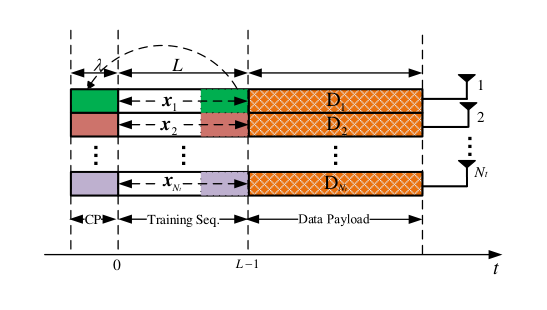
We consider a generic training-based SC-MIMO transmission structure with NtN_{t} TAs as shown in Fig. 4. It subsumes the SC-SM transmission scheme in Fig. 1 as a special case but with emphasis on the training matrix design. We assume a quasi-static frequency-selective channel where the channel impulse response (CIR) from the nn-th (1≤n≤Nt1\leq n\leq N_{t}) transmit antenna to the receiver is denoted by 𝐡n=[hn,0,hn,1,⋯,hn,λ]T\mathbf{h}_{n}=[h_{n,0},h_{n,1},\cdots,h_{n,\lambda}]^{\text{T}}, i.e., a discrete length-(λ+1)(\lambda+1) vector with hn,lh_{n,l} (0≤l≤λ0\leq l\leq\lambda) being the channel coefficient of the ll-th path. Every block at a TA is divided into two parts: training sequence followed by data payload. Let xn=[xn,0,xn,1,⋯,xn,L−1]\textit{{x}}_{n}=[x_{n,0},x_{n,1},\cdots,x_{n,L-1}] be the training sequence transmitted over the nn-th TA (1≤n≤Nt1\leq n\leq N_{t}). All the training sequences are assumed to have identical energy of EE, i.e.,

∑l=0L−1|xn,l|2=E,for all​1≤n≤Nt.\sum\limits_{l=0}^{L-1}|x_{n,l}|^{2}=E,~~\text{for all}~1\leq n\leq N_{t}. (35)

To combat ISI in a frequency-selective channel, a length-λ\lambda cyclic prefix (CP)33 3 CP-free MIMO training may be possible with certain sophisticated signal processing algorithm; however, optimal channel estimation performance in frequency-selective channel may not be straightforward due to ISI. is placed at the front of xm\textit{{x}}_{m} which is comprised of the last λ\lambda elements of xn\textit{{x}}_{n}, i.e., [xn,L−λ+2,xn,L−λ+3,⋯,xn,L−1][x_{n,L-\lambda+2},x_{n,L-\lambda+3},\cdots,x_{n,L-1}].

Refer to caption
Fig. 4: Generic training-based SC-MIMO transmission structure with NtN_{t} transmit antennas.

The kk-th received signal at a RA can be written as

yk=∑n=1Nt∑l=0λhn,l​xn,k−l+wk,y_{k}=\sum\limits_{n=1}^{N_{t}}\sum\limits_{l=0}^{\lambda}h_{n,l}x_{n,k-l}+w_{k}, (36)

where wkw_{k} a discrete uncorrelated white complex Gaussian noise sample with zero-mean and variance σw2/2\sigma^{2}_{w}/2 per dimension. To proceed, let

𝐗n=[xn,0xn,L−1⋯xn,L−λxn,1xn,0⋯xn,L−λ+1⋱xn,L−1xn,L−2⋯xn,L−λ−1]L×(λ+1),𝐡=[𝐡1𝐡2𝐡Nt]Nt​(λ+1)×1,\begin{split}\mathbf{X}_{n}=&\left[\begin{matrix}x_{n,0}&x_{n,L-1}&\cdots&x_{n,L-\lambda}\\ x_{n,1}&x_{n,0}&\cdots&x_{n,L-\lambda+1}\\ \vdots&\vdots&\ddots&\vdots\\ x_{n,L-1}&x_{n,L-2}&\cdots&x_{n,L-\lambda-1}\end{matrix}\right]_{L\times(\lambda+1)},\\ \mathbf{h}=&\left[\begin{matrix}\mathbf{h}_{1}\\ \mathbf{h}_{2}\\ \vdots\\ \mathbf{h}_{N_{t}}\end{matrix}\right]_{N_{t}(\lambda+1)\times 1},\end{split} (37)

and

𝐲=[y0,y1,⋯,yL−1]T,𝐗=[𝐗1,𝐗2,⋯,𝐗Nt]L×(Nt​λ+Nt),𝐰=[w0,w1,⋯,wL−1].\begin{split}\mathbf{y}&=[y_{0},y_{1},\cdots,y_{L-1}]^{\text{T}},\\ \mathbf{X}&=[\mathbf{X}_{1},\mathbf{X}_{2},\cdots,\mathbf{X}_{N_{t}}]_{L\times(N_{t}\lambda+N_{t})},\\ \mathbf{w}&=[w_{0},w_{1},\cdots,w_{L-1}].\end{split} (38)

Note that 𝐗n\mathbf{X}_{n} in (37) is a Toeplitz matrix in which every column is a cyclically-shifted version of xn\textit{{x}}_{n} and thus has identical energy of EE. It can be readily shown that (36) is equivalent to the following matrix equation.

𝐲=𝐗𝐡+𝐰.\mathbf{y}=\mathbf{X}\mathbf{h}+\mathbf{w}. (39)

Applying the least-squares (LS) channel estimator (unbiased), the estimated CIR vector is given by

𝐡^=(𝐗H​𝐗)−1​𝐗H​𝐲,\hat{\mathbf{h}}=\left(\mathbf{X}^{\text{H}}\mathbf{X}\right)^{-1}\mathbf{X}^{\text{H}}\mathbf{y}, (40)

and the normalized MSE can be derived as

MSE=1(Nt​λ+Nt)Tr(𝔼{(𝐡−𝐡^)(𝐡−𝐡^)H})=σw2(Nt​λ+Nt)Tr((𝐗H𝐗)−1).\begin{split}\text{MSE}&=\frac{1}{(N_{t}\lambda+N_{t})}\text{Tr}\left(\mathbb{E}\left\{\Bigl({\mathbf{h}}-\hat{\mathbf{h}}\Bigl)\Bigl({\mathbf{h}}-\hat{\mathbf{h}}\Bigl)^{\text{H}}\right\}\right)\\ &=\frac{\sigma^{2}_{w}}{(N_{t}\lambda+N_{t})}\text{Tr}\left(\Bigl(\mathbf{X}^{\text{H}}\mathbf{X}\Bigl)^{-1}\right).\end{split} (41)

(41) indicates that the minimum MSE is achieved if and only if 𝐗H​𝐗\mathbf{X}^{\text{H}}\mathbf{X} is a diagonal matrix whose elements on the diagonal are identical44 4 The proof of this statement can be found in the Appendix of [48].. Note that

𝐗H​𝐗=[𝐗1H​𝐗1𝐗1H​𝐗2⋯𝐗1H​𝐗Nt𝐗2H​𝐗1𝐗2H​𝐗2⋯𝐗2H​𝐗Nt⋱𝐗NtH​𝐗1𝐗NtH​𝐗2⋯𝐗NtH​𝐗Nt](Nt​λ+Nt)×(Nt​λ+Nt).\begin{split}&\mathbf{X}^{\text{H}}\mathbf{X}\\ =&\left[\begin{matrix}\mathbf{X}_{1}^{\text{H}}\mathbf{X}_{1}&\mathbf{X}_{1}^{\text{H}}\mathbf{X}_{2}&\cdots&\mathbf{X}^{\text{H}}_{1}\mathbf{X}_{N_{t}}\\ \mathbf{X}^{\text{H}}_{2}\mathbf{X}_{1}&\mathbf{X}_{2}^{\text{H}}\mathbf{X}_{2}&\cdots&\mathbf{X}^{\text{H}}_{2}\mathbf{X}_{N_{t}}\\ \vdots&\vdots&\ddots&\vdots\\ \mathbf{X}^{\text{H}}_{N_{t}}\mathbf{X}_{1}&\mathbf{X}_{N_{t}}^{\text{H}}\mathbf{X}_{2}&\cdots&\mathbf{X}^{\text{H}}_{N_{t}}\mathbf{X}_{N_{t}}\\ \end{matrix}\right]_{(N_{t}\lambda+N_{t})\times(N_{t}\lambda+N_{t})}.\end{split} (42)

Thus, the minimum MSE is achieved if and only if

𝐗iH​𝐗j={E​𝐈λ+1,if​i=j,𝟎(λ+1)×(λ+1),if​i≠j,\mathbf{X}^{\text{H}}_{i}\mathbf{X}_{j}=\begin{cases}E\mathbf{I}_{\lambda+1},~&\text{if}~i=j,\\ \mathbf{0}_{(\lambda+1)\times(\lambda+1)},~&\text{if}~i\neq j,\end{cases} (43)

with which we have

minimum MSE=σw2E.\text{minimum MSE}=\frac{\sigma^{2}_{w}}{E}. (44)

Relating (43) to the PCC between xi\textit{{x}}_{i} and xj\textit{{x}}_{j}, we assert that the minimum MSE is achieved if and only if

ϕ⁡(xi,xj)​(τ)={E,ifi=j,τ=0,0,ifi≠j,0≤τ≤λ,ori=j,1≤τ≤λ.\phi(\textit{{x}}_{i},\textit{{x}}_{j})(\tau)=\begin{cases}E,~~&\text{if}~i=j,\tau=0,\\ 0,~~&\text{if}~i\neq j,0\leq\tau\leq\lambda,\\ &~~~~~~~\text{or}~i=j,1\leq\tau\leq\lambda.\end{cases} (45)
Remark 3

From here onwards, (45) is referred to as the optimal condition of SM training sequences under LS channel estimator.

IV-B Proposed Training Framework For Broadband SM Systems

To uncover the optimal training sequence criteria for broadband SM systems, we define the following training matrix 𝛀\Omega.

𝛀=[x1x2xNt]=[x1,0x1,1⋯x1,L−1x2,0x2,1⋯x2,L−1⋱xNt,0xNt,1⋯xNt,L−1]Nt×L.{\text{\mbox{\boldmath{$\Omega$}}}}=\left[\begin{matrix}\textit{{x}}_{1}\\ \textit{{x}}_{2}\\ \vdots\\ \textit{{x}}_{N_{t}}\end{matrix}\right]=\left[\begin{matrix}x_{1,0}&x_{1,1}&\cdots&x_{1,L-1}\\ x_{2,0}&x_{2,1}&\cdots&x_{2,L-1}\\ \vdots&\vdots&\ddots&\vdots\\ x_{N_{t},0}&x_{N_{t},1}&\cdots&x_{N_{t},L-1}\end{matrix}\right]_{N_{t}\times L}. (46)
Remark 4

In SM system, only one TA is activated over every time-slot, hence 𝛀\Omega should be a sparse matrix in which each column has one non-zero entry only (see Example 1). This implies that each training sequence xn\textit{{x}}_{n} (1≤n≤Nt1\leq n\leq N_{t}) has Q≡L/NtQ\equiv L/N_{t} non-zero entries and (Nt−1)​Q(N_{t}-1)Q zeros. In this paper, we are concerned with non-zero entries having identical magnitude of 1 (i.e., unimodular) and therefore, each training sequence has energy of E=QE=Q.

Suppose that 𝛀\Omega has the following sparse structure.

𝛀=[T0​(𝐚1​𝟎1×(Nt−1)​Q)TQ​(𝐚2​𝟎1×(Nt−1)​Q)T(Nt−1)​Q​(𝐚Nt​𝟎1×(Nt−1)​Q)]Nt×L,{\text{\mbox{\boldmath{$\Omega$}}}}=\left[\begin{matrix}T^{0}\left(\mathbf{a}_{1}\mathbf{0}_{1\times(N_{t}-1)Q}\right)\\ T^{Q}\left(\mathbf{a}_{2}\mathbf{0}_{1\times(N_{t}-1)Q}\right)\\ \vdots\\ T^{(N_{t}-1)Q}\left(\mathbf{a}_{N_{t}}\mathbf{0}_{1\times(N_{t}-1)Q}\right)\\ \end{matrix}\right]_{N_{t}\times L}, (47)

where 𝐚n=[an,0,an,1,⋯,an,Q]\mathbf{a}_{n}=[a_{n,0},a_{n,1},\cdots,a_{n,Q}] (1≤n≤Nt1\leq n\leq N_{t}) are row vectors having identical length of QQ and energy of EE. Noted that 𝛀\Omega is obtained by vertical concatenation of NtN_{t} sparse sequences, each of which is a shifted version of a non-zero sequence in {𝐚1,𝐚2,⋯,𝐚Nt}\{\mathbf{a}_{1},\mathbf{a}_{2},\cdots,\mathbf{a}_{N_{t}}\} padded with (Nt−1)​Q(N_{t}-1)Q zeros.

An example of training matrix 𝛀\Omega having Nt=4N_{t}=4 and L=4​QL=4Q is shown below.

𝛀=[𝐚1𝟎𝟎𝟎𝟎𝐚2𝟎𝟎𝟎𝟎𝐚3𝟎𝟎𝟎𝟎𝐚4]4×4​Q,{\text{\mbox{\boldmath{$\Omega$}}}}=\left[\begin{matrix}\mathbf{a}_{1}&\mathbf{0}&\mathbf{0}&\mathbf{0}\\ \mathbf{0}&\mathbf{a}_{2}&\mathbf{0}&\mathbf{0}\\ \mathbf{0}&\mathbf{0}&\mathbf{a}_{3}&\mathbf{0}\\ \mathbf{0}&\mathbf{0}&\mathbf{0}&\mathbf{a}_{4}\end{matrix}\right]_{4\times 4Q}, (48)

where 𝟎\mathbf{0} in (48) denotes 𝟎1×Q\mathbf{0}_{1\times Q}. One can easily show that ϕ⁡(xi,xj)​(1)\phi(\textit{{x}}_{i},\textit{{x}}_{j})(1) is non-zero and therefore, the condition in (45) can only be satisfied if λ=0\lambda=0, i.e., flat-fading channels. This means that the training matrix in (48) cannot achieve minimum channel estimation MSE [see (44)] in a frequency-selective channel.

To circumvent the above problem, we propose training matrix 𝛀\Omega which takes the following structure.

𝛀=[Ω1,Ω2,⋯,ΩJ],Ωj=[T0​(𝐚1j​𝟎1×(Nt−1)​θ)Tθ​(𝐚2j​𝟎1×(Nt−1)​θ)T(Nt−1)​θ​(𝐚Mj​𝟎1×(Nt−1)​θ)]Nt×Nt​θ,\begin{split}{\text{\mbox{\boldmath{$\Omega$}}}}&=\Bigl[\Omega_{1},\Omega_{2},\cdots,\Omega_{J}\Bigl],\\ \Omega_{j}&=\left[\begin{matrix}T^{0}\left(\mathbf{a}^{j}_{1}\mathbf{0}_{1\times(N_{t}-1)\theta}\right)\\ T^{\theta}\left(\mathbf{a}^{j}_{2}\mathbf{0}_{1\times(N_{t}-1)\theta}\right)\\ \vdots\\ T^{(N_{t}-1)\theta}\left(\mathbf{a}^{j}_{M}\mathbf{0}_{1\times(N_{t}-1)\theta}\right)\\ \end{matrix}\right]_{N_{t}\times N_{t}\theta},\end{split} (49)

where 1≤j≤J,,J≥21\leq j\leq J,,J\geq 2, each unimodular row vector 𝐚nj=[an,0j,an,1j,⋯,an,θ−1j]\mathbf{a}^{j}_{n}=[a^{j}_{n,0},a^{j}_{n,1},\cdots,a^{j}_{n,\theta-1}] (1≤j≤J,1≤n≤Nt1\leq j\leq J,1\leq n\leq N_{t}) has length of θ\theta. Clearly Nt​J​θ=LN_{t}J\theta=L and Q=J​θ=L/NtQ=J\theta=L/N_{t}. The rationale is that each TA will send QQ non-zero entries over JJ sub-blocks (where J≥2J\geq 2) so that they can work in a cooperative way to enable the resultant training matrix to meet the optimal condition specified in (45).

We also define matrix 𝚿\Psi, which is obtained by removing all the zero vectors and cyclic-shift operators in 𝛀\Omega, as follows.

𝚿=[𝐚11𝐚12⋯𝐚1J𝐚21𝐚22⋯𝐚2J⋱𝐚Nt1𝐚Nt2⋯𝐚NtJ]Nt×Q.{\text{\mbox{\boldmath{$\Psi$}}}}=\left[\begin{matrix}\mathbf{a}^{1}_{1}&\mathbf{a}^{2}_{1}&\cdots&\mathbf{a}^{J}_{1}\\ \mathbf{a}^{1}_{2}&\mathbf{a}^{2}_{2}&\cdots&\mathbf{a}^{J}_{2}\\ \vdots&\vdots&\ddots&\vdots\\ \mathbf{a}^{1}_{N_{t}}&\mathbf{a}^{2}_{N_{t}}&\cdots&\mathbf{a}^{J}_{N_{t}}\end{matrix}\right]_{N_{t}\times Q}. (50)

One can see that 𝛀\Omega can be one-to-one mapped to 𝚿\Psi and vice versa. As such, 𝚿\Psi is called the characteristic matrix of the training matrix 𝛀\Omega. In the sequel, we sometimes write the training matrix and characteristic matrix as (Nt,J,θ)(N_{t},J,\theta)-𝛀\Omega and (Nt,J,θ)(N_{t},J,\theta)-𝚿\Psi, respectively.

Example 7

Training matrix (4,2,θ)(4,2,\theta)-𝛀\Omega for channel estimation in SM with 4 TAs is shown in Fig. 5. This training matrix and its characteristic matrix can be written as follows.

𝛀=[𝐚11𝟎𝟎𝟎𝐚12𝟎𝟎𝟎𝟎𝐚21𝟎𝟎𝟎𝐚22𝟎𝟎𝟎𝟎𝐚31𝟎𝟎𝟎𝐚32𝟎𝟎𝟎𝟎𝐚41𝟎𝟎𝟎𝐚42]4×8​θ,𝚿=[𝐚11𝐚12𝐚21𝐚22𝐚31𝐚32𝐚41𝐚42]4×2​θ,\begin{split}{\text{\mbox{\boldmath{$\Omega$}}}}&=\left[\begin{array}[]{cccc:cccc}\mathbf{a}^{1}_{1}&\mathbf{0}&\mathbf{0}&\mathbf{0}\hfil\lx@intercol\vrule\lx@add@cssclass&\mathbf{a}^{2}_{1}&\mathbf{0}&\mathbf{0}&\mathbf{0}\\ \mathbf{0}&\mathbf{a}^{1}_{2}&\mathbf{0}&\mathbf{0}\hfil\lx@intercol\vrule\lx@add@cssclass&\mathbf{0}&\mathbf{a}^{2}_{2}&\mathbf{0}&\mathbf{0}\\ \mathbf{0}&\mathbf{0}&\mathbf{a}^{1}_{3}&\mathbf{0}\hfil\lx@intercol\vrule\lx@add@cssclass&\mathbf{0}&\mathbf{0}&\mathbf{a}^{2}_{3}&\mathbf{0}\\ \mathbf{0}&\mathbf{0}&\mathbf{0}&\mathbf{a}^{1}_{4}\hfil\lx@intercol\vrule\lx@add@cssclass&\mathbf{0}&\mathbf{0}&\mathbf{0}&\mathbf{a}^{2}_{4}\end{array}\right]_{4\times 8\theta},\\ {\text{\mbox{\boldmath{$\Psi$}}}}&=\left[\begin{matrix}\mathbf{a}^{1}_{1}&\mathbf{a}^{2}_{1}\\ \mathbf{a}^{1}_{2}&\mathbf{a}^{2}_{2}\\ \mathbf{a}^{1}_{3}&\mathbf{a}^{2}_{3}\\ \mathbf{a}^{1}_{4}&\mathbf{a}^{2}_{4}\end{matrix}\right]_{4\times 2\theta},\end{split} (51)

where 𝟎\mathbf{0} in 𝛀\Omega stands for 𝟎1×θ\mathbf{0}_{1\times\theta}.

Refer to caption
Fig. 5: Training matrix 𝛀\Omega with Nt=4,J=2,L=2​Nt​θN_{t}=4,J=2,L=2N_{t}\theta.

Note that in frequency-selective channels, the non-zero component sequences in row 1 and row 2 tend to interfere due to multi-path propagation, likewise for row 2 and row 3, row 3 and row 4, row 4 and row 1, so on and so forth. We will show later that such interference can be mitigated by the “tail-end ZACZ” and “tail-end ZCCZ” properties of a CZCP (see Fig. 2). Also, the ISI of each row can be mitigated by the “front-end ZACZ” property of CZCP. This makes CZCP a key component in the SM training design.

Optimal SM Training Design Criteria: Assume that θ≥λ\theta\geq\lambda. Recalling (45), we assert that the optimal SM training sequences need to satisfy the following three equations55 5 Note that ϕ⁡(xi+1,xi)​(0)=0,∀1≤i<Nt\phi(\textit{{x}}_{i+1},\textit{{x}}_{i})(0)=0,~\forall~1\leq i<N_{t} and ϕ⁡(x1,xNt)​(0)=0\phi(\textit{{x}}_{1},\textit{{x}}_{N_{t}})(0)=0 can always be ensured by the proposed training matrix structure in (49)..

ϕ⁡(xi+1,xi)​(τ)=∑j=1Jρ⁡(𝐚i+1j,𝐚ij)​(θ−τ)=0,1≤τ≤λ,1≤i<Nt,\begin{split}\phi(\textit{{x}}_{i+1},\textit{{x}}_{i})(\tau)&=\sum\limits_{j=1}^{J}\rho\left({\mathbf{a}}^{j}_{i+1},{\mathbf{a}}^{j}_{i}\right)(\theta-\tau)=0,\\ &~1\leq\tau\leq\lambda,1\leq i<N_{t},\end{split} (52)
ϕ⁡(x1,xNt)​(τ)=∑j=1Jρ⁡(𝐚1⌊j⌋J+1,𝐚Ntj)​(θ−τ)=0,1≤τ≤λ,\phi(\textit{{x}}_{1},\textit{{x}}_{N_{t}})(\tau)=\sum\limits_{j=1}^{J}\rho\left({\mathbf{a}}^{\lfloor j\rfloor_{J}+1}_{1},{\mathbf{a}}^{j}_{N_{t}}\right)(\theta-\tau)=0,~1\leq\tau\leq\lambda, (53)

and

ϕ⁡(xi)​(τ)=∑j=1Jρ⁡(𝐚ij)​(τ)=0,1≤τ≤λ,1≤i≤Nt.\phi(\textit{{x}}_{i})(\tau)=\sum\limits_{j=1}^{J}\rho\left({\mathbf{a}}^{j}_{i}\right)(\tau)=0,~1\leq\tau\leq\lambda,1\leq i\leq N_{t}. (54)

Note that (52)-(53) and (54) specify the PCC conditions and PAC condition for the rows of 𝛀\Omega, respectively. It is assumed that all the non-zero entries of characteristic matrix 𝚿\Psi are drawn from alphabet set 𝒜q\mathcal{A}_{q} (see Subsection II-A for its definition). In particular, we are interested in binary (q=2q=2) and quaternary (q=4q=4) characteristic matrices owing to their low implementation complexity in practice. We have the following remark.

Remark 5

For any qq-ary characteristic matrix with even qq, JJ should be even. This implies that any binary (q=2q=2) or quaternary (q=4q=4) characteristic matrix should have even JJ.

Proof 3

Setting τ=1\tau=1 in (52), we obtain

ϕ⁡(xi+1,xi)​(1)=∑j=1Jai+1,0j​(ai,θ−1j)∗.\phi(\textit{{x}}_{i+1},\textit{{x}}_{i})(1)=\sum\limits_{j=1}^{J}a^{j}_{i+1,0}\left(a^{j}_{i,\theta-1}\right)^{*}. (55)

It is noted that the right-hand-side of (55) is a summation of JJ entries which are drawn from 𝒜q\mathcal{A}_{q}. When qq is even, every entry ai+1,0j​(ai,θ−1j)∗a^{j}_{i+1,0}\left(a^{j}_{i,\theta-1}\right)^{*} can only be cancelled by its negation (one of the JJ entries in 𝒜q\mathcal{A}_{q}) to ensure ϕ⁡(xi+1,xi)​(1)=0\phi(\textit{{x}}_{i+1},\textit{{x}}_{i})(1)=0. Therefore, JJ must be even.

Proposed Construction: Consider a (2,2,θ)(2,2,\theta)-𝚿\Psi “seed” characteristic matrix as follows.

𝚿=[𝐚11𝐚12𝐚21𝐚22]2×2​θ.{\text{\mbox{\boldmath{$\Psi$}}}}=\left[\begin{matrix}\mathbf{a}^{1}_{1}&\mathbf{a}^{2}_{1}\\ \mathbf{a}^{1}_{2}&\mathbf{a}^{2}_{2}\end{matrix}\right]_{2\times 2\theta}. (56)

Suppose the optimal conditions specified in (52)-(54) are satisfied, i.e.,

ρ⁡(𝐚21,𝐚11)​(θ−τ)+ρ⁡(𝐚22,𝐚12)​(θ−τ)=0,1≤τ≤λ,\rho\left({\mathbf{a}}^{1}_{2},{\mathbf{a}}^{1}_{1}\right)(\theta-\tau)+\rho\left({\mathbf{a}}^{2}_{2},{\mathbf{a}}^{2}_{1}\right)(\theta-\tau)=0,~1\leq\tau\leq\lambda, (57)
ρ⁡(𝐚12,𝐚21)​(θ−τ)+ρ⁡(𝐚11,𝐚22)​(θ−τ)=0,1≤τ≤λ,\rho\left({\mathbf{a}}^{2}_{1},{\mathbf{a}}^{1}_{2}\right)(\theta-\tau)+\rho\left({\mathbf{a}}^{1}_{1},{\mathbf{a}}^{2}_{2}\right)(\theta-\tau)=0,~1\leq\tau\leq\lambda, (58)

and

ρ⁡(𝐚i1)​(τ)+ρ⁡(𝐚i2)​(τ)=0,1≤τ≤λ,i∈{1,2}.\rho\left({\mathbf{a}}^{1}_{i}\right)(\tau)+\rho\left({\mathbf{a}}^{2}_{i}\right)(\tau)=0,~1\leq\tau\leq\lambda,i\in\{1,2\}. (59)

Based on the (2,2,θ)(2,2,\theta)-𝚿\Psi given in (56), we obtain an enlarged (Nt,2,θ)(N_{t},2,\theta)-characteristic matrix (Nt≥2N_{t}\geq 2 even) as follows.

𝚿~=𝟏Nt/2×1⊗Ψ=[𝟏Nt/2×1⊗𝐚11𝟏Nt/2×1⊗𝐚12𝟏Nt/2×1⊗𝐚21𝟏Nt/2×1⊗𝐚22]Nt×2​θ.\begin{split}\widetilde{{\text{\mbox{\boldmath{$\Psi$}}}}}&=\mathbf{1}_{N_{t}/2\times 1}\otimes\Psi\\ &=\left[\begin{array}[]{c:c}\mathbf{1}_{N_{t}/2\times 1}\otimes\mathbf{a}^{1}_{1}\hfil\lx@intercol\vrule\lx@add@cssclass&\mathbf{1}_{N_{t}/2\times 1}\otimes\mathbf{a}^{2}_{1}\\ \hline\cr\mathbf{1}_{N_{t}/2\times 1}\otimes\mathbf{a}^{1}_{2}\hfil\lx@intercol\vrule\lx@add@cssclass&\mathbf{1}_{N_{t}/2\times 1}\otimes\mathbf{a}^{2}_{2}\end{array}\right]_{N_{t}\times 2\theta}.\end{split} (60)

The corresponding training matrix of 𝚿~\widetilde{{\text{\mbox{\boldmath{$\Psi$}}}}} can be expressed as

𝛀~=[x1x2xNt/2xNt/2+1xNt]Nt×2​Nt​θ=[T0​(𝐚11​𝟎)T0​(𝐚12​𝟎)Tθ​(𝐚11​𝟎)Tθ​(𝐚12​𝟎)⋮⋮T(Nt/2−1)​θ​(𝐚11​𝟎)T(Nt/2−1)​θ​(𝐚12​𝟎)T(Nt/2)​θ​(𝐚21​𝟎)T(Nt/2)​θ​(𝐚22​𝟎)T(Nt/2+1)​θ​(𝐚21​𝟎)T(Nt/2+1)​θ​(𝐚22​𝟎)⋮⋮T(Nt−1)​θ​(𝐚21​𝟎)T(Nt−1)​θ​(𝐚22​𝟎)]Nt×2​Nt​θ,\begin{split}\widetilde{{\text{\mbox{\boldmath{$\Omega$}}}}}=&\left[\begin{matrix}\textit{{x}}_{1}\\ \textit{{x}}_{2}\\ \vdots\\ \textit{{x}}_{N_{t}/2}\\ \hline\cr\textit{{x}}_{N_{t}/2+1}\\ \vdots\\ \textit{{x}}_{N_{t}}\end{matrix}\right]_{N_{t}\times 2N_{t}\theta}\\ =&\left[\begin{array}[]{c:c}T^{0}\left(\mathbf{a}^{1}_{1}\mathbf{0}\right)\hfil\lx@intercol\vrule\lx@add@cssclass&T^{0}\left(\mathbf{a}^{2}_{1}\mathbf{0}\right)\\ T^{\theta}\left(\mathbf{a}^{1}_{1}\mathbf{0}\right)\hfil\lx@intercol\vrule\lx@add@cssclass&T^{\theta}\left(\mathbf{a}^{2}_{1}\mathbf{0}\right)\\ \vdots\hfil\lx@intercol\vrule\lx@add@cssclass&\vdots\\ T^{(N_{t}/2-1)\theta}\left(\mathbf{a}^{1}_{1}\mathbf{0}\right)\hfil\lx@intercol\vrule\lx@add@cssclass&T^{(N_{t}/2-1)\theta}\left(\mathbf{a}^{2}_{1}\mathbf{0}\right)\\ \hline\cr T^{(N_{t}/2)\theta}\left(\mathbf{a}^{1}_{2}\mathbf{0}\right)\hfil\lx@intercol\vrule\lx@add@cssclass&T^{(N_{t}/2)\theta}\left(\mathbf{a}^{2}_{2}\mathbf{0}\right)\\ T^{(N_{t}/2+1)\theta}\left(\mathbf{a}^{1}_{2}\mathbf{0}\right)\hfil\lx@intercol\vrule\lx@add@cssclass&T^{(N_{t}/2+1)\theta}\left(\mathbf{a}^{2}_{2}\mathbf{0}\right)\\ \vdots\hfil\lx@intercol\vrule\lx@add@cssclass&\vdots\\ T^{(N_{t}-1)\theta}\left(\mathbf{a}^{1}_{2}\mathbf{0}\right)\hfil\lx@intercol\vrule\lx@add@cssclass&T^{(N_{t}-1)\theta}\left(\mathbf{a}^{2}_{2}\mathbf{0}\right)\\ \end{array}\right]_{N_{t}\times 2N_{t}\theta},\end{split} (61)

where 𝟎\mathbf{0} stands for 𝟎1×(Nt−1)​θ\mathbf{0}_{1\times(N_{t}-1)\theta}. One can see that the optimal conditions in (53) and (54) can be satisfied by (58) and (59), respectively. Furthermore, by (57), we have

ϕ⁡(xNt/2+1,xNt/2)​(τ)=ρ⁡(𝐚21,𝐚11)​(θ−τ)+ρ⁡(𝐚22,𝐚12)​(θ−τ)=0,1≤τ≤λ.\begin{split}&\phi(\textit{{x}}_{N_{t}/2+1},\textit{{x}}_{N_{t}/2})(\tau)\\ =&\rho\left({\mathbf{a}}^{1}_{2},{\mathbf{a}}^{1}_{1}\right)(\theta-\tau)+\rho\left({\mathbf{a}}^{2}_{2},{\mathbf{a}}^{2}_{1}\right)(\theta-\tau)\\ =&0,~1\leq\tau\leq\lambda.\end{split} (62)

To ensure that (52) is satisfied for all the ii, we also require

ϕ⁡(xi+1,xi)​(τ)=0,∀i∈{1,2,⋯,Nt−1}∖{Nt/2},1≤τ≤λ.\phi(\textit{{x}}_{i+1},\textit{{x}}_{i})(\tau)=0,~\forall~i\in\{1,2,\cdots,N_{t}-1\}\setminus\{N_{t}/2\},~1\leq\tau\leq\lambda.

This leads to the following additional conditions which should be met by the (2,2,θ)(2,2,\theta)-𝚿\Psi “seed” characteristic matrix:

ϕ⁡(xi+1,xi)​(τ)=ρ⁡(𝐚11)​(θ−τ)+ρ⁡(𝐚12)​(θ−τ)=0,1≤i≤Nt/2−1,1≤τ≤λ.\begin{split}\phi(\textit{{x}}_{i+1},\textit{{x}}_{i})(\tau)=&~\rho\left({\mathbf{a}}^{1}_{1}\right)(\theta-\tau)+\rho\left({\mathbf{a}}^{2}_{1}\right)(\theta-\tau)\\ =&~0,~1\leq i\leq N_{t}/2-1,1\leq\tau\leq\lambda.\end{split} (63)
ϕ⁡(xi+1,xi)​(τ)=ρ⁡(𝐚21)​(θ−τ)+ρ⁡(𝐚22)​(θ−τ)=0,Nt/2+1≤i≤Nt−1,1≤τ≤λ.\begin{split}\phi(\textit{{x}}_{i+1},\textit{{x}}_{i})(\tau)=&~\rho\left({\mathbf{a}}^{1}_{2}\right)(\theta-\tau)+\rho\left({\mathbf{a}}^{2}_{2}\right)(\theta-\tau)\\ =&~0,~N_{t}/2+1\leq i\leq N_{t}-1,1\leq\tau\leq\lambda.\end{split} (64)

Let (𝐚,𝐛)(\mathbf{a},\mathbf{b}) be an (N=θ,Z=λ)(N=\theta,Z=\lambda)-CZCP which is proposed in Section III. Consider two “seed” characteristic matrices taking the following structures:

𝚿1=[𝐚𝐛𝐚𝐛]2×2​θ,𝚿2=[𝐚𝐛𝐛¯∗−𝐚¯∗]2×2​θ.{\text{\mbox{\boldmath{$\Psi$}}}}_{1}=\left[\begin{matrix}\mathbf{a}&\mathbf{b}\\ \mathbf{a}&\mathbf{b}\end{matrix}\right]_{2\times 2\theta},~~{\text{\mbox{\boldmath{$\Psi$}}}}_{2}=\left[\begin{matrix}\mathbf{a}&\mathbf{b}\\ \underline{\mathbf{b}}^{*}&-\underline{\mathbf{a}}^{*}\end{matrix}\right]_{2\times 2\theta}. (65)

One can readily show that (57)-(59) and (63)-(64) can be satisfied by both 𝚿1{\text{\mbox{\boldmath{$\Psi$}}}}_{1} and 𝚿2{\text{\mbox{\boldmath{$\Psi$}}}}_{2}. The resultant “seed” characteristic matrices will allow us to design training matrices (Nt,2,θ)(N_{t},2,\theta)-𝛀~\widetilde{{\text{\mbox{\boldmath{$\Omega$}}}}} [see (61)] for optimal channel estimation in SM system with NtN_{t} TAs.

Based on (Nt,2,θ)​-​𝛀~(N_{t},2,\theta)\text{-}\widetilde{{\text{\mbox{\boldmath{$\Omega$}}}}}, we can also construct a training matrix (Nt,J,θ)(N_{t},J,\theta)-𝛀¯\overline{{\text{\mbox{\boldmath{$\Omega$}}}}} (with longer row sequences and hence larger value of EE and enhanced channel estimation performance) by the following expansion rule.

𝛀¯=𝟏1×J/2⊗𝛀~,for​J>2.\overline{{\text{\mbox{\boldmath{$\Omega$}}}}}=\mathbf{1}_{1\times J/2}\otimes\widetilde{{\text{\mbox{\boldmath{$\Omega$}}}}},~\text{for}~J>2. (66)

Finally, based on (56), (60), (61), (66), we summarize the proposed SM training design as follows.

(θ,λ)​-CZCP↦(2,2,θ)​-𝚿↦(Nt,2,θ)​-​𝚿~↦(Nt,2,θ)​-​𝛀~↦(Nt,J,θ)​-​𝛀¯.\begin{split}&(\theta,\lambda)\text{-CZCP}\mapsto(2,2,\theta)\text{-}{\text{\mbox{\boldmath{$\Psi$}}}}\mapsto(N_{t},2,\theta)\text{-}\widetilde{{\text{\mbox{\boldmath{$\Psi$}}}}}\\ &~~~\mapsto(N_{t},2,\theta)\text{-}\widetilde{{\text{\mbox{\boldmath{$\Omega$}}}}}\mapsto(N_{t},J,\theta)\text{-}\overline{{\text{\mbox{\boldmath{$\Omega$}}}}}.\end{split} (67)

One may choose (Nt,2,θ)​-​𝛀~(N_{t},2,\theta)\text{-}\widetilde{{\text{\mbox{\boldmath{$\Omega$}}}}} or (Nt,J,θ)​-​𝛀¯(N_{t},J,\theta)\text{-}\overline{{\text{\mbox{\boldmath{$\Omega$}}}}} (J>2J>2) as the SM training matrix depends on the channel estimation MSE requirement which is determined by E=J​θE=J\theta [see (44)].

IV-C Numerical Evaluation

In this subsection, we evaluate the proposed SM training sequences over frequency-selective channels. Throughout this subsection, we assume Nt=4,Nr=1N_{t}=4,N_{r}=1. Consider a (λ+1)(\lambda+1)-path channel (separated by integer symbol durations) having uniform power delay profile as follows:

h⁡[t]=∑n=0λhi​δ​[t−n​T],h[t]=\sum_{n=0}^{\lambda}h_{i}\delta[t-nT], (68)

where hih_{i}’s are complex-valued Gaussian random variables with zero mean and 𝔼⁡(|hi|2)=1\mathbb{E}(|h_{i}|^{2})=1.

Let us consider the perfect (N=8,Z=4)(N=8,Z=4)-CZCP given in Table I. As we will see, (𝐚,𝐛)(\mathbf{a},\mathbf{b}) leads to optimal SM training matrix provided that the number of multi-paths is not greater than Z+1Z+1 (i.e., 5). Based on the training matrix expansion rule in (61) and applying seed characteristic matrices 𝚿1{\text{\mbox{\boldmath{$\Psi$}}}}_{1} and 𝚿2{\text{\mbox{\boldmath{$\Psi$}}}}_{2} given in (65), respectively, we obtain training matrices (4,2,8)(4,2,8)-𝛀~1\widetilde{{\text{\mbox{\boldmath{$\Omega$}}}}}_{1} and (4,2,8)(4,2,8)-𝛀~2\widetilde{{\text{\mbox{\boldmath{$\Omega$}}}}}_{2} as follows.

𝛀~1=[𝐚𝟎𝟎𝟎𝐛𝟎𝟎𝟎𝟎𝐚𝟎𝟎𝟎𝐛𝟎𝟎𝟎𝟎𝐚𝟎𝟎𝟎𝐛𝟎𝟎𝟎𝟎𝐚𝟎𝟎𝟎𝐛],𝛀~2=[𝐚𝟎𝟎𝟎𝐛𝟎𝟎𝟎𝟎𝐚𝟎𝟎𝟎𝐛𝟎𝟎𝟎𝟎𝐛¯∗𝟎𝟎𝟎−𝐚¯∗𝟎𝟎𝟎𝟎𝐛¯∗𝟎𝟎𝟎−𝐚¯∗],\begin{split}\widetilde{{\text{\mbox{\boldmath{$\Omega$}}}}}_{1}&=\left[\begin{array}[]{cccc:cccc}\mathbf{a}&\mathbf{0}&\mathbf{0}&\mathbf{0}\hfil\lx@intercol\vrule\lx@add@cssclass&\mathbf{b}&\mathbf{0}&\mathbf{0}&\mathbf{0}\\ \mathbf{0}&\mathbf{a}&\mathbf{0}&\mathbf{0}\hfil\lx@intercol\vrule\lx@add@cssclass&\mathbf{0}&\mathbf{b}&\mathbf{0}&\mathbf{0}\\ \mathbf{0}&\mathbf{0}&\mathbf{a}&\mathbf{0}\hfil\lx@intercol\vrule\lx@add@cssclass&\mathbf{0}&\mathbf{0}&\mathbf{b}&\mathbf{0}\\ \mathbf{0}&\mathbf{0}&\mathbf{0}&\mathbf{a}\hfil\lx@intercol\vrule\lx@add@cssclass&\mathbf{0}&\mathbf{0}&\mathbf{0}&\mathbf{b}\end{array}\right],\\ \widetilde{{\text{\mbox{\boldmath{$\Omega$}}}}}_{2}&=\left[\begin{array}[]{cccc:cccc}\mathbf{a}&\mathbf{0}&\mathbf{0}&\mathbf{0}\hfil\lx@intercol\vrule\lx@add@cssclass&\mathbf{b}&\mathbf{0}&\mathbf{0}&\mathbf{0}\\ \mathbf{0}&\mathbf{a}&\mathbf{0}&\mathbf{0}\hfil\lx@intercol\vrule\lx@add@cssclass&\mathbf{0}&\mathbf{b}&\mathbf{0}&\mathbf{0}\\ \mathbf{0}&\mathbf{0}&\underline{\mathbf{b}}^{*}&\mathbf{0}\hfil\lx@intercol\vrule\lx@add@cssclass&\mathbf{0}&\mathbf{0}&-\underline{\mathbf{a}}^{*}&\mathbf{0}\\ \mathbf{0}&\mathbf{0}&\mathbf{0}&\underline{\mathbf{b}}^{*}\hfil\lx@intercol\vrule\lx@add@cssclass&\mathbf{0}&\mathbf{0}&\mathbf{0}&-\underline{\mathbf{a}}^{*}\end{array}\right],\end{split} (69)

where 𝟎\mathbf{0} in (69) stands for 𝟎1×8\mathbf{0}_{1\times 8}. Taking one SM training matrix in (69) and following the expansion rule in (66), we can obtain (4,6,8)(4,6,8)-𝛀¯\overline{{\text{\mbox{\boldmath{$\Omega$}}}}} and (4,18,8)(4,18,8)-𝛀¯\overline{{\text{\mbox{\boldmath{$\Omega$}}}}}. As a comparison, we consider binary random (but regular and sparse) training matrices in which each row (of a training matrix) contains 2​λ​J2\lambda J, where J∈{2,6,18}J\in\{2,6,18\}, non-zero entries and each column consists of one non-zero entry only. Note that a larger value of JJ leads to higher value of training sequence energy EE and hence better channel estimation performance66 6 In practice, however, a longer training sequence will give rise to a higher training overhead. Hence, selection of the training length (determined by JJ) is a trade-off between channel estimation performance and training overhead.. A new random training matrix is generated for every different SM channel estimation (i.e., random on-the-fly). Following Section IV, LS channel estimator is employed. Fig. 6-a compares the channel estimation MSEs versus “EbNo (dB) per TA” for the above two types of training sequences (where J=2,6,18J=2,6,18) with frequency-selective fading channel consisting of 5 multi-paths. It is seen that the MSE curves obtained from the proposed SM training sequences match with the minimum MSE curves very well for different values of JJ. Compared to the MSE curve obtained from random training sequences, about 1.5 dB gain is achieved for J=2J=2. When JJ increases, the MSE gap between these types of sequences diminishes. This is because the diagonal elements (i.e., taking identical value of E=8​JE=8J) of 𝐗H​𝐗\mathbf{X}^{\text{H}}\mathbf{X} in (41) become significantly larger than the off-diagonal ones. Consequently, 𝐗H​𝐗\mathbf{X}^{\text{H}}\mathbf{X} approaches to an identity matrix as the proposed SM training sequences can achieve.

(a) No. of multi-paths = 5, L=32​J,J∈{2,6,18},Z=4L=32J,J\in\{2,6,18\},Z=4.
(b) EbNo=16 dB and E=32E=32.
Fig. 6: MSE comparison with training matrices from other sequences.

Next, we evaluate the channel estimation MSE performances under different values of multi-paths at EbNo of 16 dB. We employ the perfect (N=16,Z=8)(N=16,Z=8)-CZCP given in Table I to generate our proposed SM training matrix with the same structure as 𝛀~1\widetilde{{\text{\mbox{\boldmath{$\Omega$}}}}}_{1} in (69), i.e., J=2J=2. We compare its channel estimation performance with SM training matrices from the length-16 GCP (which is not a CZCP)

[1,1,1,1,1,−1,−1,1,1,1,−1,−1,1,−1,1,−11,−1,1,−1,1,1,−1,−1,1,−1,−1,1,1,1,1,1],\left[\begin{matrix}1,1,1,1,1,-1,-1,1,1,1,-1,-1,1,-1,1,-1\\ 1,-1,1,-1,1,1,-1,-1,1,-1,-1,1,1,1,1,1\end{matrix}\right],

the length-31 m-sequence77 7 An m-sequence is a pseudo-random sequence whose periodic autocorrelation sidelobes take identical value of −1-1.

𝐚m=[1,−1,−1,−1,−1,1,−1,−1,1,−1,1,1,−1,−1,1,1,1,1,1,−1,−1,−1,1,1,−1,1,1,1,−1,1,−1],\begin{split}\mathbf{a}_{\text{m}}&=[1,-1,-1,-1,-1,1,-1,-1,1,-1,1,1,-1,-1,1,\\ &~~~~1,1,1,1,-1,-1,-1,1,1,-1,1,1,1,-1,1,-1],\end{split}

one length-32 CAN sequence88 8 CAN sequences are obtained by minimizing a quadratic function associated with the integrated sidelobe level (ISL) of sequences [52]. With the aid of fast Fourier transform (FFT), CAN sequences can be generated for lengths up to 10610^{6} or even longer. More sequence synthesis algorithms based on numerical optimization can be found in [53, 54, 55, 56, 57, 58, 59]. with low aperiodic autocorrelations, the length-13 Barker sequence99 9 A Barker sequence has aperiodic autocorrelation sidelobes not exceeding 1. It is widely conjectured that no binary Barker sequences exist for lengths larger than 13 [51] and hence the application of Barker sequences may not be straightforward when a large sequence length is required.

𝐚B=[1,1,1,1,1,−1,−1,1,1,−1,1,−1,1],\mathbf{a}_{\text{B}}=[1,1,1,1,1,-1,-1,1,1,-1,1,-1,1],

four length-31 Gold sequences [60] with low periodic cross-correlations, four length-32 Zadoff-Chu sequences [61] with low periodic cross-correlations, and four “random-on-the-fly” binary sequences of length-32. For the m-sequence, Gold sequences, Zadoff-Chu sequences, CAN sequence and random sequences, we adopt the training matrix structure in (48). In particular, when a single sequence (i.e., m-sequence or CAN sequence) is used as the “seed”, we set 𝐚1=𝐚2=𝐚3=𝐚4\mathbf{a}_{1}=\mathbf{a}_{2}=\mathbf{a}_{3}=\mathbf{a}_{4} in (48). For the length-13 Barker sequence, we adopt the following training matrix

[𝐚B𝟎𝟎𝟎𝐚B𝟎𝟎𝟎𝟎𝐚B𝟎𝟎𝟎𝐚B𝟎𝟎𝟎𝟎𝐚B𝟎𝟎𝟎𝐚B𝟎𝟎𝟎𝟎𝐚B𝟎𝟎𝟎𝐚B]4×10⁴.\left[\begin{array}[]{cccc:cccc}\mathbf{a}_{\text{B}}&\mathbf{0}&\mathbf{0}&\mathbf{0}\hfil\lx@intercol\vrule\lx@add@cssclass&\mathbf{a}_{\text{B}}&\mathbf{0}&\mathbf{0}&\mathbf{0}\\ \mathbf{0}&\mathbf{a}_{\text{B}}&\mathbf{0}&\mathbf{0}\hfil\lx@intercol\vrule\lx@add@cssclass&\mathbf{0}&\mathbf{a}_{\text{B}}&\mathbf{0}&\mathbf{0}\\ \mathbf{0}&\mathbf{0}&\mathbf{a}_{\text{B}}&\mathbf{0}\hfil\lx@intercol\vrule\lx@add@cssclass&\mathbf{0}&\mathbf{0}&\mathbf{a}_{\text{B}}&\mathbf{0}\\ \mathbf{0}&\mathbf{0}&\mathbf{0}&\mathbf{a}_{\text{B}}\hfil\lx@intercol\vrule\lx@add@cssclass&\mathbf{0}&\mathbf{0}&\mathbf{0}&\mathbf{a}_{\text{B}}\end{array}\right]_{4\times 104}.

For fair comparison, we normalize the energies of all the training sequences to E=32E=32. When the number of multi-paths is 9 (or less), 𝐗H​𝐗\mathbf{X}^{\text{H}}\mathbf{X} corresponding to our proposed SM training matrix is an identity matrix multiplied by the training matrix energy and therefore, our proposed SM training matrix achieves the minimum MSEs, as shown in Fig. 6-b. The same may not be achieved by training matrices from other seed sequences. As a result, their channel estimation MSEs display certain distances to the minimum MSE regardless the number of multi-paths. It is interesting to note that the second best channel estimation performance is achieved by the SM training matrix from the length-32 CAN sequence (even better than that from the length-13 Barker sequence) whose aperiodic ISL is minimized. This makes sense because a sequence with lower aperiodic ISL tends to give rise to smaller magnitudes for the off-diagonal elements of 𝐗H​𝐗\mathbf{X}^{\text{H}}\mathbf{X} and hence better channel estimation MSEs. The worst channel estimation performance is achieved by the SM training matrices from random sequences as it is in general hard to ensure small off-diagonal elements of 𝐗H​𝐗\mathbf{X}^{\text{H}}\mathbf{X}. The second worst channel estimation performance is achieved by the SM training matrices from Gold sequences. Moreover, the channel estimation MSEs corresponding to our proposed SM training matrix start to deviate from, but very close to, the minimum MSE when the number of multi-paths increases to beyond 9. In summary, our proposed SM training matrices give rise to the minimum channel estimation MSEs provided that the number of multi-paths is no greater than Z+1Z+1; when greater than Z+1Z+1, our proposed SM training matrices may still give rise to good channel estimation MSEs in the condition that 1) 𝐗H​𝐗\mathbf{X}^{\text{H}}\mathbf{X} associated to the SM training matrix has full rank and 2) the off-diagonal elements of 𝐗H​𝐗\mathbf{X}^{\text{H}}\mathbf{X} have small magnitudes.

V Conclusions

In this paper, we have proposed a new class of sequence pairs called cross-complementary pairs (CZCPs) in which every CZCP displays zero (symmetrical) aperiodic auto-correlation (AAC) sums and zero aperiodic cross-correlation (ACC) sums for certain time-shifts. Unlike Golay complementary pairs (GCPs) whose two constituent sequences must be sent over two non-interfering channels (thus only AAC sums matter in GCPs), perfect CZCPs should be designed to minimize both ISI (determined by AAC sums) and cross-interference (by ACC sums). By investigating the structural properties of CZCPs, we have found that perfect CZCPs are equivalent to a subset of GCPs whose first halves are identical and second halves have opposite polarities (See P2 in Section III). Based on this finding, we have shown by systematic constructions that perfect binary CZCPs exist for lengths 2α+1​10β​26γ2^{\alpha+1}10^{\beta}26^{\gamma}, where α,β,γ\alpha,\beta,\gamma are non-negative integers. In Definition 6, we have extended the concept of CZCP to cross Z-complementary set (CZCS) which consists of constituent sequences of two or more.

Secondly, we have shown that CZCPs play an important role in channel training sequence design of broadband spatial modulation (SM) systems. It should be noted that the existing dense training sequences for conventional MIMO systems are unapplicable in SM systems as only one transmit antenna (TA) is activated at each time-slot. By employing CZCP, we have presented a generic framework for the design of optimal SM training matrix. We have shown that these training matrices lead to minimum channel estimation mean-squared-error in quasi-static frequency-selective channels.

As a future work, more systematic constructions (e.g., recursive expansion algorithms) for CZCPs/CZCSs (perfect or non-perfect) may be designed. When a perfect CZCP/CZCS cannot be obtained, it will be interesting to know what are the almost-perfect CZCPs/CZCSs with respect to different sequence lengths and alphabet sizes. Efficient training design for generalized SM [62, 63, 64] in dispersive channels is also an interesting and challenging issue to be explored. In particular, it is worthy to investigate efficient training sequence design when the generalized SM channels are correlated [65, 66, 67, 68, 69].

Acknowledgment

The authors are deeply indebted to Prof. Pingzhi Fan at Southwest Jiaotong University for suggesting the terminology of “CZCP”. They also would like to thank anonymous reviewers for their invaluable suggestions which greatly help improve the quality of this work.

Appendix A Proofs of CZCP Properties

Proof of P1:

Proof 4

Since (𝐜,𝐝)(\mathbf{c},\mathbf{d}) is obtained by respectively dividing 𝐚\mathbf{a} by a0a_{0} and 𝐛\mathbf{b} by b0b_{0}, we have 𝐜=𝐚/a0,𝐝=𝐛/b0\mathbf{c}=\mathbf{a}/a_{0},\mathbf{d}=\mathbf{b}/b_{0}. Therefore,

ρ⁡(𝐜)​(τ)+ρ⁡(𝐝)​(τ)=1|a0|2​ρ​(𝐚)​(τ)+1|b0|2​ρ​(𝐛)​(τ).\rho(\mathbf{c})(\tau)+\rho(\mathbf{d})(\tau)=\frac{1}{|a_{0}|^{2}}\rho(\mathbf{a})(\tau)+\frac{1}{|b_{0}|^{2}}\rho(\mathbf{b})(\tau). (70)

For qq-ary CZCP (𝐚,𝐛)(\mathbf{a},\mathbf{b}), a0,b0∈𝒜qa_{0},b_{0}\in\mathcal{A}_{q} and hence |a0|2=|b0|2=1|a_{0}|^{2}=|b_{0}|^{2}=1. Thus,

ρ⁡(𝐜)​(τ)+ρ⁡(𝐝)​(τ)=ρ⁡(𝐚)​(τ)+ρ⁡(𝐛)​(τ).\rho(\mathbf{c})(\tau)+\rho(\mathbf{d})(\tau)=\rho(\mathbf{a})(\tau)+\rho(\mathbf{b})(\tau). (71)

Furthermore, since ρ⁡(𝐚)​(N−1)+ρ⁡(𝐛)​(N−1)=ρ⁡(𝐚,𝐛)​(N−1)+ρ⁡(𝐚,𝐛)​(N−1)=0\rho(\mathbf{a})(N-1)+\rho(\mathbf{b})(N-1)=\rho(\mathbf{a},\mathbf{b})(N-1)+\rho(\mathbf{a},\mathbf{b})(N-1)=0, we have

a0​aN−1∗+b0​bN−1∗=0,a0​bN−1∗+b0​aN−1∗=0.\begin{split}a_{0}a^{*}_{N-1}+b_{0}b^{*}_{N-1}&=0,\\ a_{0}b^{*}_{N-1}+b_{0}a^{*}_{N-1}&=0.\end{split} (72)

Multiplying the above two identities by b0∗,a0∗b^{*}_{0},a^{*}_{0}, respectively, we assert that a0​b0∗=a0∗​b0a_{0}b^{*}_{0}=a^{*}_{0}b_{0} which is a real number. As a result, we have

ρ⁡(𝐜,𝐝)​(τ)+ρ⁡(𝐝,𝐜)​(τ)=1b0∗​a0​ρ​(𝐚,𝐛)​(τ)+1b0​a0∗​ρ​(𝐛,𝐚)​(τ)=1b0​a0∗[ρ(𝐚,𝐛)(τ)+ρ(𝐛,𝐚)(τ)].\begin{split}\rho(\mathbf{c},\mathbf{d})(\tau)+\rho(\mathbf{d},\mathbf{c})(\tau)&=\frac{1}{b^{*}_{0}a_{0}}\rho(\mathbf{a},\mathbf{b})(\tau)+\frac{1}{b_{0}a^{*}_{0}}\rho(\mathbf{b},\mathbf{a})(\tau)\\ &=\frac{1}{b_{0}a^{*}_{0}}\Bigl[\rho(\mathbf{a},\mathbf{b})(\tau)+\rho(\mathbf{b},\mathbf{a})(\tau)\Bigl].\end{split} (73)

Recalling the two conditions specified in (13), (71) and (73) indicate that (𝐜,𝐝)(\mathbf{c},\mathbf{d}) is also qq-ary (N,λ)(N,\lambda)-CZCP (with c0=d0=1c_{0}=d_{0}=1).

By ρ⁡(𝐜)​(N−1)+ρ⁡(𝐝)​(N−1)=0\rho(\mathbf{c})(N-1)+\rho(\mathbf{d})(N-1)=0, we have

cN−1+dN−1=0.c_{N-1}+d_{N-1}=0. (74)

Based on this (i.e., c0=d0,cN−1=−dN−1c_{0}=d_{0},c_{N-1}=-d_{N-1}), we next carry out an induction for the proof of (16). Suppose that we have ci=di,cN−1−i=−dN−1−ic_{i}=d_{i},c_{N-1-i}=-d_{N-1-i} for all i∈{0,1,⋯,k−1}i\in\{0,1,\cdots,k-1\} where k≤Z−1k\leq Z-1. Next, we calculate the aperiodic correlation sums at τ=N−k−1\tau=N-k-1 which involves the correlations of the following vectors.

[𝐜1𝐜2𝐝1𝐝2]=[1c1c2⋯ck−1ckcN−k−1cN−kcN−k+1⋯cN−2cN−11d1d2⋯dk−1dkdN−k−1dN−kdN−k+1⋯dN−2dN−1].\left[\begin{matrix}\mathbf{c}_{1}\\ \mathbf{c}_{2}\\ \mathbf{d}_{1}\\ \mathbf{d}_{2}\end{matrix}\right]=\left[\begin{matrix}1&c_{1}&c_{2}&\cdots&c_{k-1}&c_{k}\\ c_{N-k-1}&c_{N-k}&c_{N-k+1}&\cdots&c_{N-2}&c_{N-1}\\ 1&d_{1}&d_{2}&\cdots&d_{k-1}&d_{k}\\ d_{N-k-1}&d_{N-k}&d_{N-k+1}&\cdots&d_{N-2}&d_{N-1}\end{matrix}\right]. (75)

Note that

ρ⁡(𝐜)​(N−k−1)+ρ⁡(𝐝)​(N−k−1)=⟨𝐜1,𝐜2⟩+⟨𝐝1,𝐝2⟩=0,\begin{split}&\rho(\mathbf{c})(N-k-1)+\rho(\mathbf{d})(N-k-1)\\ =&\Bigl<\mathbf{c}_{1},\mathbf{c}_{2}\Bigl>+\Bigl<\mathbf{d}_{1},\mathbf{d}_{2}\Bigl>=0,\end{split} (76)
ρ⁡(𝐜,𝐝)​(N−k−1)+ρ⁡(𝐝,𝐜)​(N−k−1)=⟨𝐜1,𝐝2⟩+⟨𝐝1,𝐜2⟩=0.\begin{split}&\rho(\mathbf{c},\mathbf{d})(N-k-1)+\rho(\mathbf{d},\mathbf{c})(N-k-1)\\ =&\Bigl<\mathbf{c}_{1},\mathbf{d}_{2}\Bigl>+\Bigl<\mathbf{d}_{1},\mathbf{c}_{2}\Bigl>=0.\end{split} (77)

By (75), we have

cN−k−1∗+∑i=1kci​cN−k−1+i∗+dN−k−1∗+∑i=1kdi​dN−k−1+i∗=0,c^{*}_{N-k-1}+\sum\limits_{i=1}^{k}c_{i}c^{*}_{N-k-1+i}+d^{*}_{N-k-1}+\sum\limits_{i=1}^{k}d_{i}d^{*}_{N-k-1+i}=0, (78)

and

dN−k−1∗+∑i=1kci​dN−k−1+i∗+cN−k−1∗+∑i=1kdi​cN−k−1+i∗=0.d^{*}_{N-k-1}+\sum\limits_{i=1}^{k}c_{i}d^{*}_{N-k-1+i}+c^{*}_{N-k-1}+\sum\limits_{i=1}^{k}d_{i}c^{*}_{N-k-1+i}=0. (79)

Summing up (78) and (79), we have

2​(cN−k−1∗+dN−k−1∗)+∑i=1kci​(cN−k−1+i∗+dN−k−1+i∗⏟=0)+∑i=1kdi(cN−k−1+i∗+dZ−k−1+i∗⏟=0)=0.\begin{split}&2(c^{*}_{N-k-1}+d^{*}_{N-k-1})+\sum\limits_{i=1}^{k}c_{i}\left(\underbrace{c^{*}_{N-k-1+i}+d^{*}_{N-k-1+i}}_{=0}\right)\\ &~~~+\sum\limits_{i=1}^{k}d_{i}\left(\underbrace{c^{*}_{N-k-1+i}+d^{*}_{Z-k-1+i}}_{=0}\right)=0.\end{split} (80)

Subtracting (78) by (79), we have

(ck−dk)​cN−1∗+∑i=1k−1(ci−di⏟=0)​cN−k−1+i∗−(ck−dk)​dN−1∗+∑i=1k−1(di−ci⏟i=0)d∗Z−k−1+i=0.\begin{split}&(c_{k}-d_{k})c^{*}_{N-1}+\sum\limits_{i=1}^{k-1}\left(\underbrace{c_{i}-d_{i}}_{=0}\right)c^{*}_{N-k-1+i}-(c_{k}-d_{k})d^{*}_{N-1}\\ &~~~+\sum\limits_{i=1}^{k-1}\left(\underbrace{d_{i}-c_{i}}_{i=0}\right)d^{*}_{Z-k-1+i}=0.\end{split} (81)

By (80), we have cN−k−1=−dN−k−1c_{N-k-1}=-d_{N-k-1}. By (81) and considering cN−1≠dN−1c_{N-1}\neq d_{N-1}1010 10 Otherwise, we have cN−1=dN−1=0c_{N-1}=d_{N-1}=0 by cN−1+dN−1=0c_{N-1}+d_{N-1}=0. This contradicts with the precondition that (𝐜,𝐝)(\mathbf{c},\mathbf{d}) is a qq-ary CZCP., we assert that ck=dkc_{k}=d_{k}. Continuing this induction, the proof of (16) follows.

Next, we assume Z>N/2Z>N/2 and NN is even. Setting i=N/2−1i=N/2-1 into (16), we have cN/2+dN/2=0c_{N/2}+d_{N/2}=0. Then, setting i=N/2i=N/2 into (16), we obtain cN/2=dN/2c_{N/2}=d_{N/2}. This requires that cN/2=dN/2=0c_{N/2}=d_{N/2}=0 which contradicts with the precondition that (𝐜,𝐝)(\mathbf{c},\mathbf{d}) is a qq-ary CZCP. When NN is odd, another contradiction is reached for c(N−1)/2=d(N−1)/2=0c_{(N-1)/2}=d_{(N-1)/2}=0. In either case, we assert that Z≤N/2Z\leq N/2 should be met.

Proof of P2:

Proof 5

In Section II, we have shown that if (𝐚,𝐛)(\mathbf{a},\mathbf{b}) is a GCP, (𝐛¯∗,−𝐚¯∗)(\underline{\mathbf{b}}^{*},-\underline{\mathbf{a}}^{*}) will also be a GCP which is mutually orthogonal to (𝐚,𝐛)(\mathbf{a},\mathbf{b}). The first identity of (32) is similar to the mutually orthogonal property of GCPs, although with some slight changes for its proof. Here, we only prove the second equality of (32). For 1≤τ≤Z1\leq\tau\leq Z, we have

ρ⁡(𝐛,𝐛¯∗)​(N−τ)+ρ⁡(𝐚,−𝐚¯∗)​(N−τ)=∑i=0τ−1(bibτ−1−i−aiaτ−1−i).\begin{split}&\rho(\mathbf{b},\underline{\mathbf{b}}^{*})(N-\tau)+\rho(\mathbf{a},-\underline{\mathbf{a}}^{*})(N-\tau)\\ =&\sum\limits_{i=0}^{\tau-1}\Bigl(b_{i}b_{\tau-1-i}-a_{i}a_{\tau-1-i}\Bigl).\end{split} (82)

By assumption, we have ai=bi,aN−1−i=−bN−1−i,for all​i∈(𝒯1−1)a_{i}=b_{i},a_{N-1-i}=-b_{N-1-i},~\text{for all}~i\in(\mathcal{T}_{1}-1). Thus, the above equation reduces to

ρ⁡(𝐛,𝐛¯∗)​(N−τ)+ρ⁡(𝐚,−𝐚¯∗)​(N−τ)=∑i=0τ−1ai(bτ−1−i−aτ−1−i⏟=0)=0.\begin{split}&\rho(\mathbf{b},\underline{\mathbf{b}}^{*})(N-\tau)+\rho(\mathbf{a},-\underline{\mathbf{a}}^{*})(N-\tau)\\ =&\sum\limits_{i=0}^{\tau-1}a_{i}\Bigl({\underbrace{b_{\tau-1-i}-a_{\tau-1-i}}_{=0}}\Bigl)=0.\end{split} (83)

On the other hand, when τ=Z+1\tau=Z+1, we have

ρ⁡(𝐛,𝐛¯∗)​(N−τ)+ρ⁡(𝐚,−𝐚¯∗)​(N−τ)=∑i=1λ−1ai(bZ−i−aZ−i⏟=0)+2a0(bZ−aZ⏟≠0)≠0.\begin{split}&\rho(\mathbf{b},\underline{\mathbf{b}}^{*})(N-\tau)+\rho(\mathbf{a},-\underline{\mathbf{a}}^{*})(N-\tau)\\ =&\sum\limits_{i=1}^{\lambda-1}a_{i}\Bigl({\underbrace{b_{Z-i}-a_{Z-i}}_{=0}}\Bigl)+2a_{0}(\underbrace{b_{Z}-a_{Z}}_{\neq 0})\neq 0.\end{split} (84)

This proves the second equality of (32).

Proof of P3:

Proof 6

For binary sequence pair (𝐚,𝐛)(\mathbf{a},\mathbf{b}) over {−1,1}\{-1,1\}, by the first condition specified in (13), we have

ρ⁡(𝐚)​(N−1)+ρ⁡(𝐛)​(N−1)=a0​aN−1+b0​bN−1=0.\rho\left(\mathbf{a}\right)(N-1)+\rho\left(\mathbf{b}\right)(N-1)=a_{0}a_{N-1}+b_{0}b_{N-1}=0. (85)

Also, we require

ρ⁡(𝐚)​(1)+ρ⁡(𝐛)​(1)=∑i=0N−2(ai​ai+1+bi​bi+1)=0.\rho\left(\mathbf{a}\right)(1)+\rho\left(\mathbf{b}\right)(1)=\sum\limits_{i=0}^{N-2}(a_{i}a_{i+1}+b_{i}b_{i+1})=0. (86)

Let ai=1−2​a~i,bi=1−2​b~ia_{i}=1-2\tilde{a}_{i},b_{i}=1-2\tilde{b}_{i}, where 1≤i≤N1\leq i\leq N and a~i,b~i∈ℤ2\tilde{a}_{i},\tilde{b}_{i}\in\mathbb{Z}_{2}. Consequently, (85) and (86), respectively, imply that

a~0+a~N−1+b~0+b~N−1=1​(mod​2),\tilde{a}_{0}+\tilde{a}_{N-1}+\tilde{b}_{0}+\tilde{b}_{N-1}=1~(\text{mod}~2), (87)

and

N−1=∑i=0N−2(ai+ai+1+bi+bi+1)​(mod​2)=a~0+a~N−1+b~0+b~N−1​(mod​2).\begin{split}N-1&=\sum\limits_{i=0}^{N-2}(a_{i}+a_{i+1}+b_{i}+b_{i+1})~(\text{mod}~2)\\ &=\tilde{a}_{0}+\tilde{a}_{N-1}+\tilde{b}_{0}+\tilde{b}_{N-1}~(\text{mod}~2).\end{split} (88)

Combining (87) and (88), we assert that NN should be an even positive integer.

In the end, (18) of P3 can be easily obtained by an induction exploiting ρ​(𝐚)​(τ)+ρ​(𝐛)​(τ)\rho\left(\mathbf{a}\right)(\tau)+\rho\left(\mathbf{b}\right)(\tau) starting from τ=N−1\tau=N-1 to τ=N−Z\tau=N-Z. This induction is similar to that in [2, 14] and therefore detailed proof of (18) is omitted.

References

  • [1] M. J. E. Golay, “Statatic multislit spectroscopy and its application to the panoramic display of infrared spectra,” J. Opt. Soc. Amer., vol. 41, pp. 468-472, 1951.
  • [2] M. J. E. Golay, “Complementary series,” IRE Trans. Inf. Theory, vol. IT-7, pp. 82-87, Apr. 1961.
  • [3] S. Budišin, “New complementary pairs of sequences,” Electron. Lett., vol. 26, no. 13, pp. 881-883, Jun. 1990.
  • [4] S. Budišin, “New multilevel complementary pairs of sequences,” Electron. Lett., vol. 26, no. 22, pp. 1861-1863, Oct. 1990.
  • [5] S. Budišin and P. Spasojevíc, “Paraunitary generation/correlation of QAM complementary sequence pairs,” in Proc. Cryptography Commun., vol. 6, no. 1, pp. 59-102, Oct. 2014.
  • [6] Z. Wang, G. Wu, and D. Ma, “A new method to construct Golay complementary set by paraunitary matrices and Hadamard matrices,” in Proc. 9th International Conference on Sequences and Their Applications (SETA-2016), Sep. 2016, pp. 1-12.
  • [7] S. Das, S. Budišin, S. Majhi, Z. Liu, and Y. L. Guan, “A multiplier-free generator for polyphase complete complementary codes,” IEEE Trans. Signal Process., vol. 66, no. 5, pp. 1184-1192, Mar. 2018.
  • [8] S. Budišin and P. Spasojevíc, “Paraunitary-based Boolean generator for QAM complementary sequences of length 2K2^{K},” IEEE Trans. Inf. Theory, vol. 64, no. 8, pp. 5938-5956, Aug. 2018.
  • [9] J. A. Davis and J. Jedwab, ”Peak-to-mean power control in OFDM, Golay complementary sequences, and Reed-Muller codes,” IEEE Trans. Inf. Theory, vol. 45, no. 7, pp. 2397-2417, Nov. 1999.
  • [10] Y. Li, “A construction of general QAM Golay complementary sequences,” IEEE Trans. Inf. Theory, vol. 56, no. 11, pp. 5765-5771, Nov. 2010.
  • [11] Z. Liu, Y. Li, and Y. L. Guan, “New constructions of general QAM Golay complementary sequences,” IEEE Trans. Inf. Theory, vol. 59, no. 11, pp. 7684-7692, Nov. 2013.
  • [12] P. Fan and M. Darnell, Sequence Design for Communications Applications. New York: Wiley, 1996.
  • [13] M. G. Parker, K. G. Paterson, and C. Tellambura, “Golay complementary sequences,” Wiley Encyclopedia of Telecommunications, J. G. Proakis, Ed. New York: Wiley Interscience, 2002.
  • [14] Z. Liu, U. Parampalli, and Y. L. Guan, “Optimal odd-length binary Z-complementary pairs,” IEEE Trans. Inf. Theory, vol. 60, no. 9, pp. 5768-5781, July 2014.
  • [15] P. Fan, W. Yuan, and Y. Tu, “Z-complementary binary sequences,” IEEE Signal Process. Lett., vol. 14, pp. 401-404, Aug. 2007.
  • [16] C. Tseng and C. Liu, “Complementary sets of sequences,” IEEE Trans. Inf. Theory, vol. IT-18, pp. 644-665, Sept. 1972.
  • [17] A. Rathinakumar and A. K. Chaturvedi, “Complete mutually orthogonal Golay complementary sets from Reed-Muller codes,” IEEE Trans. Inf. Theory, vol. 54, pp. 1339-1346, Mar. 2008.
  • [18] S. Wang and A. Abli, “Aperiodic complementary sets of sequences-based MIMO frequency selective channel estimation,” IEEE Commun. Lett., vol. 9, no. 10, pp. 891-893, Oct. 2005.
  • [19] S. Wang and A. Abdi, “MIMO ISI channel estimation using uncorrelated Golay complementary sets of polyphase sequences,” IEEE Trans. Veh. Tech., vol. 56, pp. 3024-3040, Sep. 2007.
  • [20] S. Z. Budišin, “Efficient pulse compressor for Golay complementary sequences,” IEE Electron. Lett., vol. 27, pp. 219-220, Jan. 1991.
  • [21] A. Pezeshki, A. R. Calderbank, W. Moran, and S. D. Howard, “Doppler resilient Golay complementary waveforms,” IEEE Trans. Inf. Theory, vol. 54, pp. 4254-4266, Sep. 2008.
  • [22] H. H. Chen, J. F. Yeh, and N. Seuhiro, “A multicarrier CDMA architecture based on orthogonal complementary codes for new generations of wideband wireless communications,” IEEE Commun. Magazine, vol. 39, pp. 126-135, Oct. 2001.
  • [23] H. H. Chen, The Next Generation CDMA Techonolgies, John Wiley & Sons, Jul. 2007.
  • [24] Z. Liu, Y. L. Guan, and H. H. Chen, “Fractional-delay-resilient receiver for interference-free MC-CDMA communications based on complete complementary codes,” IEEE Trans. Wireless Commun., vol. 14, no. 3, pp. 1226-1237, Mar. 2015.
  • [25] B. M. Popović, “Synthesis of power efficient multitone signals with flat amplitude spectrum,” IEEE Trans. Commun., vol. 39, pp. 1031-1033, Jul. 1991.
  • [26] K. G. Paterson, “Generalized Reed-Muller codes and power control in OFDM modulation,” IEEE Trans. Inf. Theory, vol. 46, pp. 104-120, Jan. 2000.
  • [27] Z. Liu, Y. L. Guan, and U. Parampalli, “New complete complementary codes for the peak-to-mean power control in MC-CDMA,” IEEE Trans. Commun., vol. 62, pp. 1105-1113, Mar. 2014.
  • [28] E. Telatar, “Capacity of multi-antenna Gaussian channels,” Eur. Trans. Telecommun., vol. 10, no. 6, pp. 585-595, Nov./Dec. 1999.
  • [29] V. Tarokh, H. Jafarkhani, and A. R. Calderbank, “Space-time block codes from orthogonal designs,” IEEE Trans. Inf. Theory, vol. 45, no. 5, pp. 1456-1467, Jul. 1999.
  • [30] B. Hassibi and B. M. Hochwald, “High-rate codes that are linear in space and time,” IEEE Trans. Inf. Theory, vol. 48, no. 7, pp. 1804-1824, Jul. 2002.
  • [31] L. Zheng and D. N. C. Tse, “Diversity and multiplexing: A fundamental tradeoff in multiple-antenna channels,” IEEE Trans. Inf. Theory, vol. 49, no. 5, pp. 1073-1096, May 2003.
  • [32] J. Mietzner, R. Schober, L. Lampe, W. H. Gerstacker, and P. A. Höeher, “Multiple-antenna techniques for wireless communications-A comprehensive literature survey,” IEEE Commun. Surveys Tuts., vol. 11, no. 2, pp. 87-105, Second Quart., 2009.
  • [33] E. Basar, “On multiple-input multiple-output OFDM with index modulation for next generation wireless networks,” IEEE Trans. Signal Process., vol. 64, no. 15, pp. 3868-3878, Aug. 2016.
  • [34] B. Zheng, M. Wen, E. Basar, and F. Chen, “Multiple-input multipleoutput OFDM with index modulation: Low-complexity detector design,” IEEE Trans. Signal Process., vol. 65, no. 11, pp. 2758-2772, Jun. 2017.
  • [35] R. Mesleh, H. Haas, Y. Lee, and S. Yun, “Interchannel interference avoidance in MIMO transmission by exploiting spatial information,” in Proc. 16th IEEE Int. Symp. PIMRC, Berlin, Germany, 2005, vol. 1, pp. 141-145.
  • [36] R. Mesleh, H. Haas, S. Sinanovi, C. W. Ahn, and S. Yun, “Spatial modulation,” IEEE Trans. Veh. Technol., vol. 57, no. 4, pp. 2228-2241, Jul. 2008.
  • [37] M. Di Renzo, H. Haas, and P. M. Grant, “Spatial modulation for multiple antenna wireless systems: A survey,” IEEE Commun. Mag., vol. 49, no. 12, pp. 182-191, Dec. 2011.
  • [38] P. Yang, M. D. Renzo, Y. Xiao, S. Li, and L. Hanzo, “Design guidlines for spatial modulation,” IEEE Commun. Surveys Tuts., vol. 17, no. 1, pp. 6-26, First Quart., 2015.
  • [39] M. Wen, B. Zheng, K. Kim, M. Renzo, T. Tsiftsis, K.-C. Chen, and N. Al-Dhahir, “A survey on spatial modulation in emerging wireless systems: research progresses and applications,” IEEE J. Sel. Areas Commun., vol. 37, no. 9, pp. 1949-1972, Sep. 2019.
  • [40] P. Yang, Y. Xiao, Y. L. Guan, K. V. S. Hari, A. Chockalingam, S. Sugiura, H. Hass, M. D. Renzo, C. Masouros, Z. Liu, L. Xiao, S. Li, and L. Hanzo, “Single-carrier SM-MIMO: a promising design for broadband large-scale antenna systems,” IEEE Commun. Surveys Tuts., vol. 18, no. 3, pp. 1687-1716, Third Quart., 2016.
  • [41] J. Jeganathan, A. Ghrayeb, and L. Szczecinski, “Spatial modulation: Optimal detection and performance analysis,” IEEE Commun. Lett., vol. 12, no. 8, pp. 545-547, Aug. 2008.
  • [42] M. D. Renzo and H. Haas, “Bit error probability of SM-MIMO over generalized fading channels,” IEEE Trans. Veh. Technol., vol. 61, no. 3, pp. 1124-1144, Mar. 2012.
  • [43] E. Basar, U. Aygolu, E. Panayirci, and H. Poor, “Performance of spatial modulation in the presence of channel estimation errors,” IEEE Commun. Lett., vol. 16, no. 2, pp. 176-179, Feb. 2012.
  • [44] M. Di Renzo, D. De Leonardis, F. Graziosi, and H. Haas, “Space shift keying (SSK-) MIMO with practical channel estimates,” IEEE Trans. Commun., vol. 60, no. 4, pp. 998-1012, Apr. 2012.
  • [45] S. Sugiura and L. Hanzo, “Effects of channel estimation on spatial modulation,” IEEE Signal Process. Lett., vol. 19, no. 12, pp. 805-808, Dec. 2012.
  • [46] X. Wu, H. Claussen, M. Renzo, and H. Hass, “Channel estimation for spatial modulation,” IEEE Trans. Commun., vol. 62, no. 12, pp. 4362-4372, Dec. 2014.
  • [47] C. Fragouli, N. Al-Dhahir, and W. Turin, “Training-based channel estimation for multiple-antenna broadband transmissions,” IEEE Trans. Wireless Commun., vol. 2, no. 2, pp. 384-391, Mar. 2003.
  • [48] S. A. Yang and J. Wu, “Optimal binary training sequence design for multiple-antenna systems over dispersive fading channels,” IEEE Trans. Veh. Technol., vol. 51, pp. 1271-1276, Sept. 2002.
  • [49] C. Fragouli, N. Al-Dhahir, and W. Turin, “Training-based channel estimation for multiple-antenna broadband transmissions,” IEEE Trans. Wireless Commun., vol. 2, no. 2, pp. 384-391, Mar. 2003.
  • [50] P. Fan and W. H. Mow, “On optimal training sequence design for multiple-antenna systems over dispersive fading channels and its extensions,” IEEE Trans. Veh. Technol., vol. 53, no. 5, pp. 1623-1626, Sep. 2004.
  • [51] P. Borwein and M. J. Mossinghoff, “Barker sequences and flat polynomials”, in Number Theory and Polynomials, Cambridge University Press, pp. 71–88, 2008.
  • [52] P. Stoica, H. He, and J. Li, “New algorithms for designing unimodular sequences with good correlation properties,” IEEE Trans. Signal Process., vol. 57, no. 4, pp. 1415-1425, Apr. 2009.
  • [53] M. Soltanalian and P. Stoica, “Computational design of sequences with good correlation properties,” IEEE Trans. Signal Process., vol. 60, no. 5, pp. 2180-2193, May 2012.
  • [54] M. Soltanalian and P. Stoica, “Designing unimodular codes via quadratic optimization,” IEEE Trans. Signal Process., vol. 62, no. 5, pp. 1221-1234, Mar. 2014.
  • [55] J. Song, P. Babu, and D. Palomar, “Optimization methods for designing sequences with low autocorrelation sidelobes,” IEEE Trans. Signal Process., vol. 63, no. 15, pp. 3998-4009, Aug. 2015.
  • [56] Y. Sun, P. Babu, and D. P. Palomar, “Majorization-minimization algorithms in signal processing, communications, and machine learning,” IEEE Trans. Signal Process., vol. 65, no. 3, pp. 794-816, Feb. 2017.
  • [57] M. A. Kerahroodi, A. Aubry, A. De Maio, M. M. Naghsh, and M. Modarres-Hashemi, “A coordinate-descent framework to design low PSL/ISL sequences,” IEEE Trans. Signal Process., vol. 65, no. 22, pp. 5942-5956, Nov. 2017.
  • [58] M. Alaee-Kerahroodi, M. R. Bhavani Shankar, K. V. Mishra, and B. Ottersten, “Meeting the lower bound on designing set of unimodular sequences with small aperiodic/periodic ISL,” in 2019 20th International Radar Symposium (IRS), pp. 1-13, Jun. 2019.
  • [59] M. Alaee-Kerahroodi, M. Modarres-Hashemi, and M. M. Naghsh, “Designing sets of binary sequences for MIMO radar systems,” IEEE Trans. Signal Process., vol. 67, no. 13, pp. 3347-3360, Jul. 2019.
  • [60] R. Gold, “Maximal recursive sequences with 3-valued recursive cross-correlation functions,” IEEE Trans. Inf. Theory, vol. 14, pp. 154-156, Jan. 1968.
  • [61] D. Chu, “Polyphase codes with good periodic correlation properties (Corresp.),” IEEE Trans. Inf. Theory, vol. IT-18, no. 4, pp. 531-532, Jul. 1972.
  • [62] J. Fu, C. Hou, W. Xiang, L. Yan, and Y. Hou, “Generalised spatial modulation with multiple active transmit antennas,” in Proc. IEEE GLOBECOM Workshops, Dec. 2010, pp. 839-844.
  • [63] T. Datta and A. Chockalingam, “On generalized spatial modulation,” in Proc. IEEE Wireless Commun. Netw. Conf. (WCNC’2013), Apr. 2013, pp. 2716-2721.
  • [64] J. Wang, S. Jia, and J. Song, “Generalised spatial modulation system with multiple active transmit antennas and low complexity detection scheme,” IEEE Trans.Wireless Commun., vol. 11, no. 4, pp. 1605-1615, Apr. 2012.
  • [65] Y. Liu, T. Wong, and W. Hager, “Training signal design for estimation of correlated MIMO channels with colored interference,” IEEE Trans. Signal Process., vol. 55, no. 4, pp. 1486-1497, Apr. 2007.
  • [66] D. Katselis, E. Kofidis, and S. Theodoridis, “On training optimization for estimation of correlated MIMO channels in the presence of multiuser interference”, IEEE Trans. Signal Process., vol. 56, no. 10, pp. 4892-4904, Oct. 2008.
  • [67] M. Biguesh, S. Gazor, and M. Shariat, “Optimal training sequence for MIMO wireless systems in colored environments”, IEEE Trans. Signal Process., vol. 57, no. 8, pp. 3144-3153, Aug. 2009.
  • [68] E. Bjornson and B. Ottersten, “A framework for training-based estimation in arbitrarily correlated Rician MIMO channels with Rician disturbance”, IEEE Trans. Signal Process., vol. 58, no. 3, pp. 1807-1820, Mar. 2010.
  • [69] N. Shariati, J. Wang and M. Bengtsson,“Robust training sequence design for correlated MIMO channel estimation”, IEEE Trans. Signal Process., vol. 62, no. 1, pp. 107-120, Jan. 2014.