The Impossibility of Efficient Quantum Weak Coin-Flipping

In the current paper, we prove the following lower bound on the number of communication rounds for quantum weak coin-flipping (see Theorem 8.2):

This result shows that, at least in the standard model, practical quantum weak coin-flipping with vanishing bias is not feasible.

The proof of this result builds on previous techniques, including the concept of a valid time-independent point game (abbreviated as “valid TIPG”). A valid TIPG is a pair of real-valued functions $m_{1},m_{2}$ on $\mathbb{R}_{\geq 0}\times\mathbb{R}_{\geq 0}$ that satisfy a certain infinite set of linear constraints (see subsections 3.2–3.3). It is known that any weak coin-flipping protocol determines a valid TIPG, and vice versa. This correspondence was used to prove the family of protocols with vanishing bias in [19]. Here I prove a negative result: any TIPG obtained from a weak coin-flipping protocol with small bias must have very large $1$-norm — i.e., $\left\|m_{1}\right\|_{1}+\left\|m_{2}\right\|_{1}$ must be very large as a function of $\epsilon$. Since there is a relationship between the number of communication rounds of a protocol and the $1$-norms of its associated time-independent point games, this implies the main result.

Ambainis’s original bound [4] of $\Omega(\log\log(1/\epsilon))$ was based on a more direct study of quantum weak coin-flipping protocols: he performed an inductive argument, using the fidelity function, on the intermediate states arising in the protocol. This approach appears to be fairly different from the one in this paper, although it may be possible to relate the two.

Theorem 1.1 is a further step in mapping out the full range of cryptographic possibilities in a two-party quantum setting (see [7, 24] for surveys on this topic). A number of other negative results are known: secure two-party computation (under certain definitions) is impossible [13, 8], and strong coin-flipping [12, 9], bit commitment [14, 16, 9], and oblivious transfer [13, 10] are all impossible except with fixed positive bias. This paper shows that the case of quantum weak coin-flipping is different: it can be achieved with arbitrarily small bias, but it is impossible to do so in polynomial time.

Certainly, this is not the end of the story. The model for quantum weak coin flipping makes a number of assumptions, including that the players exchange information in discrete stages, and that they are completely unconstrained in their ability to manipulate any quantum systems that are not under the control of the other player. This impossibility result gives us additional motivation to study coin-flipping in other settings, including relativistic models.

Sections 2–3 of this paper cover preliminaries and known material, and then new contributions appear in sections 4–8. In section 4, I define the profile of a time-independent point game, which is a two-variable function associated to a time-independent point game that distills some of its most relevant information. Sections 5–6 prove some mathematical lemmas, including a key result on the behavior of highly concentrated rational functions (Proposition 5.3). Section 7 proves the result about the $1$-norm of a time-independent point game using tools from the previous sections. Finally, section 8 proves Theorem 1.1. I conclude by noting some further directions in section 9.

I am grateful to Aarthi Sundaram (my co-author on a companion project) for many interesting discussions about the coin-flipping literature which helped to seed some of the ideas contained here. This paper also owes a large debt to Alexandre Eremenko, who showed me the complex analysis method that I used to prove Proposition 5.3. Thanks to Gorjan Alagic, Jonathan Katz, Yi-Kai Liu, and Scott Wolpert for their help with this project, and to Michael Newman for giving me an introduction to [1] some years ago.

This work is a contribution of the U. S. National Institute of Standards and Technology (NIST), and is not subject to copyright in the United States. Any mention of commercial products is for information purposes only, and does not imply endorsement by NIST.

We briefly cover some complex analysis tools that will be important in section 5. The reader can consult [3] for more details.

Let $\mathbb{C}$ denote the set of complex numbers. We will apply addition and multiplication to $\mathbb{C}\cup\left\{\infty\right\}$ using natural rules ($c+\infty=\infty,1/\infty=0$, etc.). For any $z\in\mathbb{C}$ and $r\geq 0$, let

(The set $\mathbb{D}(z,r)$ is the open disc of radius $r$ centered at $z$, and the set $\mathbb{S}(z,r)$ is the circle of radius $r$ centered at $z$.) When $z=0$ and $r=1$, we may write these sets simply as $\mathbb{D}$ and $\mathbb{S}$. Also let

If $Y\subseteq\mathbb{C}\cup\{\infty\}$, then $\overline{Y}$ denotes the closure of $Y$. For ease of notation we will write $\overline{\mathbb{D}}(z,r)$ for the closure of $\mathbb{D}(z,r)$. Let $\overline{\mathbb{H}}$ denote the set $\left\{z\in\mathbb{C}\mid\textnormal{Im }z\geq 0\right\}\cup\{\infty\}$.

If $S\subseteq\mathbb{C}$ is an open set, then a function $f\colon S\to\mathbb{C}$ is analytic if for any $p\in S$, $f$ can be expressed as a power series on some open neighborhood of $p$. If $f$ is analytic and $\overline{\mathbb{D}}(z,r)$ is a closed disc within its domain, then the following equation always holds:

The definition of a weak coin flipping protocol (which we will first sketch, and then state formally) is intended to capture a general situation where two parties with competing interests are trying to fairly flip a coin. There are two possible outcomes: $0$ (or “heads”) which is the desired outcome for Alice, and $1$ (or “tails”) which is the desired outcome for Bob. There is no trusted third party in the protocol, and thus it consists entirely of communication between Alice and Bob. At the end of the protocol, the parties report bits $a$ and $b$ respectively (representing what they ostensibly believe to be the outcome of the coin flip).

The protocol is accomplished by Alice and Bob passing a quantum system (represented by the finite-dimensional Hilbert space $\mathcal{M}$) back and forth between them, while keeping private systems (represented by $\mathcal{A}$ and $\mathcal{B}$) to themselves. In each odd round $i$, Alice performs a unitary operator $U_{i}$ on $\mathcal{A}\mathcal{M}$ followed by a binary projective measurement $\left\{E_{i},I_{\mathcal{AM}}-E_{i}\right\}$ on $\mathcal{AM}$. If the latter measurement fails — that is, if its postmeasurement state is not in $\textnormal{Supp }E_{i}$ — then Alice aborts the protocol and simply reports her favored outcome $0$. (This event is understood to mean that Alice has stopped because she suspects cheating.) On even rounds, Bob does analogous operations with operators $U_{i},E_{i}$ on $\mathcal{MB}$. At the end of the protocol, if neither party has aborted, they each perform a binary projective measurement on their private system and report the result (as $a$ and $b$, respectively). The definition requires that if Alice and Bob behave honestly in the protocol, then the probability that $a=b=0$ is $1/2$, and the probability that $a=b=1$ is $1/2.$

For the definition above, the states

for $i\in\{1,\ldots,n-1\}$, are referred to as the intermediate states of the protocol.

Let us suppose that Bob (whose goal is to force Alice to report $a=1$) chooses to behave dishonestly in the protocol. In that case, he can apply arbitrary unitary operations $V_{2},V_{4},V_{6},\ldots$ on $\mathcal{M}\mathcal{B}$ in place of $E_{2}U_{2},E_{4}U_{4},E_{6}U_{6},\ldots$. (We do not account for any measurements performed by Bob in this case, since his own output is irrelevant.) This motivates the following definition. The cheating probability for Bob (in protocol $\mathbf{C}$) is the maximum of

over all unitary operators $V_{2},V_{4},\ldots,V_{n}$ on $\mathcal{MB}$.

Let $P_{B}^{*}$ denote the cheating probability for Bob, and let $P_{A}^{*}$ denote the cheating probability for Alice (defined analogously). Then, the bias of the weak coin-flipping protocol $\mathbf{C}$ is the quantity

Valid point games are elegant mathematical constructions which, as we will see, are in a near-perfect correspondence with weak coin-flipping protocols. Because they are a lot simpler to define, valid point games provide a convenient method of reduction for questions about weak coin-flipping protocols. We will give the definition of valid point games in this subection, and then explain their relationship to weak coin-flipping protocols in subsection 3.3. We use standard terminology with a few additions.

Given a move $q$, it can be helpful to visualize $q$ by graphing its support set $\textnormal{Supp }q$ and writing out the values $q(x,y)$ associated to each point $(x,y)\in\textnormal{Supp }q$. See Figure 2 for an example of a move whose support is of size $5$.

A time-dependent point game is, roughly speaking, a finite sequence of two-dimensional configurations $z_{0},\ldots,z_{n}$. However, for mathematical convenience, we define time-dependent point games in terms of the moves $(z_{i}-z_{i-1})$ rather than the configurations $z_{i}$. Recall that for any real-valued function $f$, we write $f^{+}$ and $f^{-}$ for the positive and negative parts of $f$, respectively.

In the above definition, we refer to $\left(\sum_{i=1}^{n}m_{i}\right)^{-}$ as the initial configuration of $M$, and we refer to $\left(\sum_{i=1}^{n}m_{i}\right)^{+}$ as the final configuration of $M$. The configurations on the left side of inequality (15) are referred to as the intermediate configurations of $M$. The support of a point game $M$, denoted $\textnormal{Supp }M$, is the union of the supports of the moves in $M$.

Next we will define valid moves.

(We note that condition (18) is actually redundant, since it can be proved from (17).) Equivalently, a move is valid if and only if its inner product with any operator monotone function is nonnegative (see subsection 3.2 of [1]). We note the following useful fact, which is easily proved from Definition 3.5.

For any two-dimensional move $q$, the rows of $q$ are the functions of the form $x\mapsto q(x,y)$ (for $y\in\mathbb{R}_{\geq 0}$) and the columns of $q$ are the functions of the form $y\mapsto q(x,y)$ (for $x\in\mathbb{R}_{\geq 0}$).

For later use, we define the concept of a time-independent point game, which is simply a sequence of two-dimensional moves with no restrictions on nonnegativity (unlike Definition 3.4). In this paper, as in previous papers on weak coin-flipping, it is only useful to consider time-independent point games that involve $2$ moves, and so we confine our definition accordingly.

We apply the term “valid” to time-independent point games in the obvious way: a time-independent point game $(m_{1},m_{2})$ is valid if $m_{1}$ is horizontally valid and $m_{2}$ is vertically valid. Note that any time-dependent point game $(m_{1},\ldots,m_{n})$ yields a time-independent point game

and the latter game is valid if $(m_{1},\ldots,m_{n})$ is valid.

Now we will state the known results which motivate our study of valid point games. There is a close correspondence between valid point games and weak coin-flipping protocols, and this correspondence allows us to deduce assertions about coin-flipping protocols (of both existence and impossibility) by studying properties of point games.

If $M$ is a point game from the configuration $\frac{1}{2}(\llbracket 0,1\rrbracket+\llbracket 1,0\rrbracket)$ to a single point $[\alpha,\beta]$, then we will naturally refer to the quantity $\max\{\alpha,\beta\}-1/2$ as the bias of $M$. The above theorem can be understood as asserting that if an $n$-round weak coin-flipping protocol exists with bias $\epsilon$, then there are $n$-round valid point games with bias arbitrarily close to $\epsilon$. A proof of Theorem 3.10, which is based on semidefinite programming duality, is given in [1].¹¹ 1 The proof appears in sections 1–3 in [1]. Note that the definitions of point games used by the authors in [1] are the “transpose” of ours: under their definitions, a valid point game begins with a vertically valid move rather than a horizontally valid move. (We note that Theorem 3.10 also has a converse, although we will not need it here. See Theorem 3 and Theorem 4 in [1].)

Next we assert a theorem about the relationship between weak coin-flipping protocols and time-independent point games.

We make one final note about symmetry in valid TIPGs.

We begin with the definition of the profile function in the one-dimensional case. The one-dimensional profile function can be thought of simply as a construction that bundles together the three conditions that define a valid move (Definition 3.5).

The profile function $\widehat{\ell}$ collects some useful information about $\ell$. One can easily verify from the definition that

For illustration, we give a graph of the function $P_{3}(\alpha)$ (that is, the profile of $\llbracket 3\rrbracket$) in Figure 3.

The reader will observe that there are multiple ways that the one-dimensional profile function could have been defined to achieve the property in Proposition 4.2 (e.g., using different ranges for $\alpha$ and different rational expressions). This particular choice of definition will make some of the arguments in section 7 mathematically easier. One of the reasons that this definition is convenient is that the profile of $\llbracket 1\rrbracket$ is simply the constant function $\alpha\mapsto 1$.

Next we define the profile of a two-dimensional move.

As with the one-dimensional profile, some of the values of a two-dimensional profile $\widehat{q}$ have natural expressions — for example,

and

The basic motivation to study the two-dimensional profile function is the following proposition.

As a consequence of the above proposition, if $M=(m_{1},\ldots,m_{n})$ is a valid time-dependent point game and $z_{0},z_{1},\ldots,z_{n-1},z_{n}$ are its configurations, we must have

for any $\alpha,\beta\in[1,\infty]$. The profile function gives us an infinite family of constraints that must be satisfied by the initial and final configurations of any valid point game.

We make note of some additional elementary facts for later use.

From subsection 3.3, we know that if there exists a quantum weak coin-flipping protocol whose bias is less than $\epsilon$ (with $0<\epsilon<\frac{1}{2}$), then there must exist a valid TIPG $(m_{1},m_{2})$ such that $m_{1}+m_{2}$ is equal to

We therefore have a crucial interest in the moves $v_{\epsilon}$. However, it is mathematically simpler to instead study the family of moves

for $0<\tau<1$. Note that if $\tau=4\epsilon/(1+2\epsilon)$, then

and so (using Proposition 3.6), valid TIPGs for $v_{\epsilon}$ correspond exactly to valid TIPGs for $t_{\tau}$ via the same linear transformation.

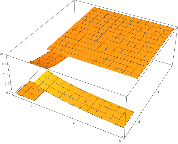
If $R=(r_{1},r_{2})$ is a valid TIPG such that $r_{1}+r_{2}=t_{\tau}$, then we must have $\widehat{r_{1}}+\widehat{r_{2}}=\widehat{t_{\tau}}$. The profile function $\widehat{t_{\tau}}$ can be expressed as follows.

A graph of an example (with $\tau=1/10$) is given in Figure 4.

We will first reproduce a standard result about the logarithm of the absolute value of an analytic function. We begin with the following observation: if $f$ is an analytic function on a neighborhood of $\overline{\mathbb{D}}$ which has no zeroes in $\overline{\mathbb{D}}$, then there is a well-defined analytic function $\log f$ on a neighborhood of $\overline{\mathbb{D}}$ such that $2^{\log f}=f$. We have (see subsection 2.1):

Since the real part of $\log f(z)$ is precisely $\log\left|f(z)\right|$, this proves the following.

For the result that we will prove in subsection 5.2, we will need a similar statement that addresses the case where $f$ is permitted to have zeroes in $\overline{\mathbb{D}}$ and may not be analytic on $\mathbb{S}$. This motivates a somewhat more intricate claim. Let us say that a real-valued function on the unit circle $\mathbb{S}$ is a step function if it is locally constant at all but a finite number of points in $\mathbb{S}$. A proof of the following proposition is given in Appendix A.1.

We will now prove the main result of this section. This result is concerned with rational functions that have real poles — that is, functions $f\colon\mathbb{C}\cup\left\{\infty\right\}\to\mathbb{C}\cup\left\{\infty\right\}$ that can be expressed in the form

where $g(z)$ is a polynomial and $c_{i}\in\mathbb{R}$. We will show that under certain assumptions, these functions must take on large values on the complex unit circle.

Recall that if $A$ and $B$ are sets and $B\subseteq A$, then we write $A\smallsetminus B$ for the set of all elements in $A$ that are not in $B$.

We illustrate the statement above with an example. Let

This function, which is graphed in Figure 5, satisfies $\left|h(0)\right|=1$ and

The quantity $\max_{\left|z\right|=1}\left|h(z)\right|$ in this case is indeed quite large (on the order of $10^{20}$).

References

- [1] Dorit Aharonov, Andre Chailloux, Maor Ganz, Iordanis Kerenidis, and Loick Magnin. A simpler proof of the existence of quantum weak coin flipping with arbitrarily small bias. SIAM Journal on Computing, 45(3):633–679, 2016.
- [2] Dorit Aharonov, Amnon Ta-Shma, Umesh V. Vazirani, and Andrew C. Yao. Quantum bit escrow. In Proceedings of the Thirty-second Annual ACM Symposium on Theory of Computing, STOC ’00, pages 705–714, New York, NY, USA, 2000. ACM.
- [3] Lars V. Ahlfors. Complex Analysis. McGraw-Hill, 3rd edition, 1979.
- [4] Andris Ambainis. A new protocol and lower bounds for quantum coin flipping. Journal of Computer and System Sciences, 68(2):398 – 416, 2004. Special Issue on STOC 2001.
- [5] Atul Singh Arora, Jérémie Roland, and Stephan Weis. Quantum weak coin flipping. In Proceedings of the 51st Annual ACM SIGACT Symposium on Theory of Computing, STOC 2019, pages 205–216, New York, NY, USA, 2019. ACM.
- [6] Manuel Blum. Coin flipping by telephone a protocol for solving impossible problems. SIGACT News, 15(1):23–27, January 1983.
- [7] Anne Broadbent and Christian Schaffner. Quantum cryptography beyond quantum key distribution. Designs, Codes and Cryptography, 78(1):351–382, Jan 2016.
- [8] Harry Buhrman, Matthias Christandl, and Christian Schaffner. Complete insecurity of quantum protocols for classical two-party computation. Phys. Rev. Lett., 109:160501, Oct 2012.
- [9] André Chailloux and Iordanis Kerenidis. Physical limitations of quantum cryptographic primitives or optimal bounds for quantum coin flipping and bit commitment. SIAM Journal on Computing, 46(5):1647–1677, 2017.
- [10] André Chailloux, Iordanis Kerenidis, and Jamie Sikora. Lower bounds for quantum oblivious transfer. Quantum Info. Comput., 13(1-2):158–177, January 2013.
- [11] Richard Cleve. Limits on the security of coin flips when half the processors are faulty. In Proceedings of the Eighteenth Annual ACM Symposium on Theory of Computing, STOC ’86, pages 364–369, New York, NY, USA, 1986. ACM.
- [12] Zeph Landau. A tensor network view of Kitaev’s lower bound for strong coin flipping. Video, available at (https://www.youtube.com/watch?v=1VYezqof_2Q). 2014.
- [13] Hoi-Kwong Lo. Insecurity of quantum secure computations. Phys. Rev. A, 56:1154–1162, Aug 1997.
- [14] Hoi-Kwong Lo and H. F. Chau. Is quantum bit commitment really possible? Phys. Rev. Lett., 78:3410–3413, Apr 1997.
- [15] Hoi-Kwong Lo and H.F. Chau. Why quantum bit commitment and ideal quantum coin tossing are impossible. Physica D: Nonlinear Phenomena, 120(1):177 – 187, 1998. Proceedings of the Fourth Workshop on Physics and Consumption.
- [16] Dominic Mayers. Unconditionally secure quantum bit commitment is impossible. Phys. Rev. Lett., 78:3414–3417, Apr 1997.
- [17] Carlos Mochon. Quantum weak coin-flipping with bias of 0.192. In 45th Annual IEEE Symposium on Foundations of Computer Science, pages 2–11, Oct 2004.
- [18] Carlos Mochon. Large family of quantum weak coin-flipping protocols. Phys. Rev. A, 72:022341, Aug 2005.
- [19] Carlos Mochon. Quantum weak coin flipping with arbitrarily small bias. arXiv:0711.4114v1, 2007.
- [20] Tal Moran, Moni Naor, and Gil Segev. An optimally fair coin toss. Journal of Cryptology, 29(3):491–513, Jul 2016.
- [21] Rolf Nevanlinna. Analytic Functions. Springer-Verlag, 1970.
- [22] R. W. Spekkens and T. Rudolph. Degrees of concealment and bindingness in quantum bit commitment protocols. Phys. Rev. A, 65:012310, Dec 2001.
- [23] R. W. Spekkens and Terry Rudolph. Quantum protocol for cheat-sensitive weak coin flipping. Phys. Rev. Lett., 89:227901, Nov 2002.
- [24] Stephanie Wehner, David Elkouss, and Ronald Hanson. Quantum internet: A vision for the road ahead. Science, 362(6412), 2018.
Appendix A Appendices
A.1 Proof of Proposition 5.2
We state some elementary facts.
Fact A.1.
If is an analytic function on an open neighborhood of a compact set , and is not the zero function, then has only a finite number of zeroes in .
Fact A.2.
If is a continuous function, then the family of functions on given by