Trust Assessment in Online Social NetworksThanks: This paper is the full version of [1], which is published in IEEE Transaction on Dependable and Secure Computing.

We model a social network as a directed graph $G=(V,E)$ where a vertex $u\in V$ represents a user, and an edge $e(u,v)\in E$ denotes a trust relation from $u$ to $v$. The weight of $e(u,v)$ denotes how much $u$ trusts $v$, which is commonly referred to as direct trust. A trustor may leverage the recommendations from other users to derive a trustee’s trust, which is called indirect trust. We are interested in computing the indirect trust between two users who have not established a direct trust previously. To solve this problem, we first need to design a trust model that works with both direct and indirect trust. Based on the assumption that trust is determined by objective evidence, designing a trust model can be stated as follows.

• •

  P1: Given the interactions between a trustor and a trustee, how to model the trust of the trustee, from the trustor’s perspective?

The second problem is to compute/infer indirect trust between users in an OSN. Solving this problem means the trust between two users, without previous interactions, can be computed. Because the indirect trust inference is available, a trustor can conduct a trust assessment of a trustee in an OSN. As such, the second problem is formulated as follows.

• •

  P2: Given a social network $G=(V,E)$, $\forall$ $u$ and $v$, s.t. $e(u,v)$ $\not\in E$ and $\exists$ at least one path from $u$ to $v$, how does one compute $u$’s trust in $v$, i.e., how should $u$ trust a stranger $v$?

To address problem P1, we propose the three-valued subjective logic (3VSL) model that accurately models the trust between a trustor and a trustee, based on their interactions. 3VSL is inspired by the subjective logic (SL) model [13], however, it is significantly different from SL.

The major difference between SL and 3VSL lies in the definitions of uncertainty in trust. SL believes the uncertainty in the trust of a trustee never changes, however, 3VSL considers the uncertainty increases as trust propagates among users in an OSN. Therefore, an extra state, called uncertainty state, is introduced in 3VSL to cope with the changing of uncertainty in trust.

The trust of a trustee, i.e., the probability that it will behave as expected, can be represented by a Dirichlet-Categorical (DC) distribution that is characterized by three parameters $\alpha$, $\beta$ and $\gamma$. Here, $\alpha$ is the number of positive interactions occurred, i.e., a trustor observed that the trustor behaved as expected for $\alpha$ times. $\beta$ denotes the amount of negative interactions, indicating the trustee did not behave as expected. It is also quite possible that the behavior of the trust is ambiguous, i.e., it is impossible to determine whether it behaved as expected or not. In this case, we consider uncertain observations are made and use $\gamma$ to record them. Uncertainty is generated not only when ambiguous behaviors are observed but also when trust propagates within an OSN, which will be elaborated in details in Section 3. The observations kept in $\alpha$, $\beta$ and $\gamma$ are also called evidence, as they are used to judge whether the trustee is trustworthy or not. The major reason of introducing the uncertain state in 3VSL is to accurately capture the trust propagation process. When trust propagates from a user to another, certain evidence in $\alpha$ and $\beta$ are “distorted” and “converted” into uncertain evidence. Given a DC distribution, it can be represented by a vector $\left<\alpha,\beta,\gamma\right>$, which is also called opinion. On the other hand, the trustee’s trust can be derived from a DC distribution; therefore, trust can be represented by an opinion. In the rest of this paper, we treat trust and opinion as interchangeable concepts, unless otherwise specified.

To address problem P2, we propose a trust assessment algorithm, called AssessTrust (AT), based on the 3VSL model. The AT algorithm decomposes the network between the trustor and trustee as a parsing tree that provides the correct order of applying trust operations to computer the indirect trust between the two users. Here, the trust operations available in trust computation are the discounting operation and combining operation. Leveraging these two operations, AT is proven to be able to accurately compute the trust between any two users connected in an OSN. Because 3VSL appropriately treats the uncertainty in trust, AT offers more accurate trust assessments, compared to the topology- and graph-based solutions. On the other hand, as AT aims at computing indirect trust between users, it outperforms the probability based models that focus only on direct trust. Experiment results demonstrate that AT achieves the most accurate trust assessment results. Specifically, AT achieves the F1 scores of $0.7$ and $0.75$, using the Advogato and Pretty Good Privacy (PGP) datasets, respectively. AT can rank users based on their trust values. We measure the accuracy of the ranking results, using the Kendall’s tau coefficients. Experiment results show that, on average, AT offers $0.73$ and $0.77$ kendall’s tau coefficients, in Advogato and PGP, respectively.

The first technical challenge is that 3VSL needs to accurately model the trust propagation and fusion in OSNs. This is a challenge because trust propagation in OSNs is not well understood, although it is widely adopted by the research community. We address this challenge by using an opinion to represent trust and modeling trust propagation based on DC distribution and several commonly-accepted assumptions.

The second technical challenge is that 3VSL must be able to work on OSNs with non-series-parallel network topologies. This is a challenge because the only allowed operations in trust assessment are trust propagation and trust fusion. However, these two operations require that a network’s topology must be either series and/or parallel. This requirement cannot be satisfied in real-world online social networks. We address this challenge by differentiating distorting opinions from original opinions. For example, if Alice trusts Bob and Bob trusts Charlie, then Alice’s opinion on Bob is called the distorting opinion, and Bob’s opinion on Charlie is the original opinion. We find that original opinions can be fused only once but distorting opinions can be combined any number of times. This discovery lays the foundation for the proposed recursive AssessTrust algorithm. The third technical challenge is that 3VSL needs to handle social networks with arbitrary topologies, even with cycles. This is a challenge because it is impossible to test 3VSL in all possible network topologies. We address this challenge by mathematically proving 3VSL works in arbitrary networks. The proof is based upon the characteristics of Dirichlet distribution and the properties of different opinions in the trust computation process. In the end, the AssessTrust algorithm is designed to compute the trust between any two users in an OSN.

The rest of this paper is organized as follows. In Section 2, the background and terminologies of trust are introduced. In Section 3, we introduce the 3VSL model and define the trust propagation and fusion operations. We then differentiate discounting opinions from original opinions in Section 4, and prove 3VSL can handle arbitrary network topologies. In the same section, we detail the proposed AssessTrust algorithm. In Section 5, we validate the 3VSL model and the AssessTrust algorithm, using two real-world datasets. The related work is given in Section 6. We conclude the paper in Section 8.

In this section, we briefly introduce some terminologies frequently referred in this paper. Trust assessment is defined as the process that a trustor assesses a trustee on whether it will perform a certain task as expected. As such, trust can be either direct or indirect [14]. Direct trust is formed from a trustor’s direct interactions with a trustee while indirect trust is inferred from others’ recommendations. Typically, trust is represented as an opinion, indicating how much a trustor trusts a trustee.

To model trust propagation and trust fusion, two opinion operations, i.e., the discounting operation and combining operation, are design to facilitate trust computation/assessment [14]. Trust fusion refers to combining different trust opinions to form a consensus trust opinion. Trust propagation refers to a trust opinion being transferred from a user to another. For example, if $A$ trusts $B$, and $B$ trusts $C$, then $B$’s opinion on $C$ will be discounted by $A$ to derive an indirect opinion of $C$’s trust.

To better understand 3VSL, we first briefly introduce the subjective logic (SL) [13]. Considering two users $A$ and $X$, $A$’s opinion on $X$’s trust can be described by an opinion.

$$\begin{array}[]{l}\omega_{AX}=\left\langle{{\alpha_{AX}},{\beta_{AX}},2}\right\rangle\left|{{a_{AX}}},\right.\end{array}$$

where $\alpha_{AX}$, $\beta_{AX}$, and $2$ denote the amounts of evidence supporting user $X$ is trustworthy, untrustworthy, and uncertain, respectively. Based on $\alpha_{AX}$ and $\beta_{AX}$, a Beta distribution can be formed to model $A$’s trust in $X$.

In SL, the amount of uncertain evidence in an opinion is always $2$. $a_{AX}$ is called the base rate and formed from existing impression without solid evidence, e.g., prejudice, preference, or a general opinion obtained from hearsay. For example, if $A$ always distrusts/trusts the users from a certain group where $X$ belongs to, then $a_{AX}$ will be smaller/greater than $0.5$. Note that the opinion in SL [13] was defined as $\omega_{AX}=\left\langle{{b_{AX}},{d_{AX}},u_{AX}}\right\rangle\left|{{a_{AX}}}\right.$, which is another form of the trust opinion. The connection between these two opinion representations is mentioned in [13] as follows.

	$\displaystyle b_{AX}=\frac{\alpha_{AX}}{\alpha_{AX}+\beta_{AX}+2}$
	$\displaystyle d_{AX}=\frac{\beta_{AX}}{\alpha_{AX}+\beta_{AX}+2}$		(2.1)
	$\displaystyle u_{AX}=\frac{2}{\alpha_{AX}+\beta_{AX}+2}$

Leveraging the property of Beta distribution, two opinions can be fused, by combining the corresponding Beta distributions, to yield a new opinion. For example, opinions ${\omega_{1}}=\left\langle{{\alpha_{1}},{\beta_{1}},2}\right\rangle\left|{{a_{1}}}\right.$ and ${\omega_{2}}=\left\langle{{\alpha_{2}},{\beta_{2}},2}\right\rangle\left|{{a_{2}}}\right.$ can be combined to produce ${\omega_{12}}=\left\langle{{\alpha_{12}},{\beta_{12}},2}\right\rangle\left|{{a_{12}}}\right.$, where $\alpha_{12}$, $\beta_{12}$ and $a_{12}$ are calculated as follows.

$\displaystyle\left\{\begin{array}[]{l}{{\alpha_{12}}={\alpha_{1}}+{\alpha_{2}}}\\ {{\beta_{12}}={\beta_{1}}+{\beta_{2}}}\\ {{a_{12}}=\displaystyle\frac{{{a_{1}}+{a_{2}}}}{2}}\end{array}.\right.$

Let $A$ and $B$ denote two users where ${\omega_{1}}=\left\langle{{\alpha_{1}},{\beta_{1}},2}\right\rangle\left|{{a_{1}}}\right.$ is $A$’s opinion about $B$’s trust. Assume $C$ is another user and ${\omega_{2}}=\left\langle{{\alpha_{2}},{\beta_{2}},2}\right\rangle\left|{{a_{2}}}\right.$ is $B$’s opinion about $C$’s trust. Then, the discounting operation is applied to compute $A$’s indirect opinion about $C$’s trust $\omega_{AC}=\left\langle{{\alpha_{12}},{\beta_{12}},2}\right\rangle\left|{{a_{12}}}\right.$ where

$\displaystyle\left\{\begin{array}[]{l}{\alpha_{12}}=\displaystyle\frac{{{\alpha_{1}}{\alpha_{2}}}}{{\left({{\beta_{2}}+{\alpha_{2}}+2}\right)\left({{\beta_{1}}+{\alpha_{1}}+2}\right)}}\cdot\frac{2}{\kappa}\\ {\alpha_{12}}=\displaystyle\frac{{{\alpha_{1}}{\beta_{2}}}}{{\left({{\beta_{2}}+{\alpha_{2}}+2}\right)\left({{\beta_{1}}+{\alpha_{1}}+2}\right)}}\cdot\frac{2}{\kappa}\\ {a_{12}}={a_{2}}\end{array},\right.$

and

$$\kappa=1-\frac{{\left({{\alpha_{1}}{\alpha_{2}}+{\alpha_{1}}{\beta_{2}}}\right)}}{{\left({{\beta_{2}}+{\alpha_{2}}+2}\right)\left({{\beta_{1}}+{\alpha_{1}}+2}\right)}}.$$

Trust in 3VSL is defined as the probability that a trustee will behave as expected in the future. The probability is determined by the amounts of evidence that a trustor observed about a trustee’s historical behaviors. A trustee may be observed behaving as expected, not expected, or in an ambiguous way. As a result, a trustor obtains positive, negative, and uncertain evidence accordingly. Based on the observed evidence, Bayesian inference is used to infer the probability of a trustee being trustworthy, or the probability that a trustee will behave as expected in the future. In summary, given more positive observed evidence, the probability of a trustee being trustworthy is larger.

The uncertainty state in 3VSL not only contains the observed uncertain evidence but also the distorted evidence when trust propagates in the network. Knowing how much evidence is distorted will give us an idea of how much positive (and negative) evidence left, which must be accurate so that the probability inference (of trust) could be precise. Without keeping track of uncertainty evidence, the amount of certain evidence in an opinion becomes incorrect, leading to erroneous trust assessments.

A trustee’s future behavior can be modeled as a random variable $x$ that takes on one of three possible outcomes $\{1,2,3\}$, i.e., $x=1$, $x=2$ and $x=3$ indicating the trustee will behave as expected, not as expected, or in an ambiguous way, respectively. As such, we are interested in the probability that $x=1$, which is determined by the positive observed behaviors of the trustee. Therefore, the probability density function (pdf) of $x$ follows the Categorical distribution.

$$f(x|\mathbf{p})=\prod_{i=1}^{3}p_{i}^{[x=i]},$$

where $\mathbf{p}=(p_{1},p_{2},p_{3})$ and $p_{1}+p_{2}+p_{3}=1$, $p_{i}$ represents the probability of observing event $i$. The Iverson bracket $[x=i]$ evaluates to 1 if $x=i$, and 0 otherwise.

If the value of $\mathbf{p}$ is available, the pdf of $x$ will be known and the probability of $x=i$ can be computed. Unfortunately, $\mathbf{p}$ is an unknown parameter and needs to be estimated based on the observations of $x$. We treat $\mathbf{p}$ as three random variables that follow the Dirichlet distribution.

$$\mathbf{p}\sim Dir(\alpha,\beta,\gamma),$$

where $\alpha,\beta,\gamma$ are hyper-parameters that control the shape of the Dirichlet distribution. We assume $\mathbf{p}$ follows Dirichlet distribution mainly because it is a conjugate prior of categorical distribution. In addition, because Dirichlet distribution belongs to a family of continuous multivariate probability distributions, we have various pdfs for $\mathbf{p}$ by changing the values of $\alpha,\beta,\gamma$.

$$f(\mathbf{p})=C{p_{1}}^{\alpha-1}{p_{2}}^{\beta-1}{p_{3}}^{\gamma-1},$$

(3.1)

where $C$ is a normalizing factor ensuring $p_{1}+p_{2}+p_{3}=1$. In this way, we use $\mathbf{p}\sim Dir(\alpha,\beta,\gamma)$ to model the uncertainty in estimating $\mathbf{p}$.

With the mathematical model in place, $\mathbf{p}$ can be estimated based on the observations of $x$, according to the Bayesian inference. Given a set of independent observations of $x$, denoted by $\mathbf{D}=\{x_{1},x_{2},\cdots,x_{n}\}$ where $x_{j}\in\{1,2,3\}$ and $j=1,2,\cdots,n$, we want to know how likely $\mathbf{D}$ is observed. This probability can be computed as

$$P(\mathbf{D}|\mathbf{p})=\prod_{j=1}^{n}p_{1}^{[x_{j}=1]}p_{2}^{[x_{j}=2]}p_{3}^{[x_{j}=3]}.$$

Let $c_{i}$ denote the number of observations where $x=i$, then the above equation becomes $p_{1}^{c_{1}}p_{2}^{c_{2}}p_{3}^{c_{3}}$. Based on Bayesian inference, given observed data $\mathbf{D}$, the posterior pdf of $\mathbf{p}$ can be estimated from

$$f(\mathbf{p}|\mathbf{D})=\frac{P(\mathbf{D}|\mathbf{p})f(\mathbf{p})}{P(\mathbf{D})},$$

where $P(\mathbf{D}|\mathbf{p})=p_{1}^{c_{1}}p_{2}^{c_{2}}p_{3}^{c_{3}}$ is the likelihood function, and $f(\mathbf{p})$ the prior pdf of $\mathbf{p}$. $P(\mathbf{D})$ is the probability that $\mathbf{D}$ is observed, which is independent of $\mathbf{p}$. Therefore, we have

$$f(\mathbf{p}|\mathbf{D})\propto p_{1}^{c_{1}}p_{2}^{c_{2}}p_{3}^{c_{3}}\times p_{1}^{\alpha-1}p_{2}^{\beta-1}p_{3}^{\gamma-1}.$$

That means the posterior pdf $f(\mathbf{p}|\mathbf{D})$ can be modeled by another Dirichlet distribution $Dir(\alpha+c_{1},\beta+c_{2},\gamma+c_{3})$. With the posterior pdf of $\mathbf{p}$, we have the following predicative model for $x$.

$$f(x|\mathbf{D})=\int f(x|\mathbf{p})f(\mathbf{p}|\mathbf{D})d\mathbf{p}.$$

(3.2)

This function is in fact a composition of Categorical ($f(x|\mathbf{p})$) and Dirichlet ($f(\mathbf{p}|\mathbf{D})$) distributions, so it is called Dirichlet-Categorical (DC) distribution [15].

In the previous section, we introduce how to model a trustee’s future behavior by a DC distribution. From a DC distribution, the probability that the trustee is trustworthy can be derived from Eq. 3.2. Because the shape of a DC distribution is determined by three parameters, we use these parameters to form a vector to represent it. This vector is called opinion that expresses a trustor’s opinion about a trustee’s trust.

For a given DC distribution, the only undetermined parameters are $\alpha,\beta,\gamma$. We set $\alpha=\beta=\gamma=1$, if there is no observed data, i.e., $\mathbf{D}=\emptyset$. In this case, the DC distribution yields a uniform distribution, i.e., $p_{1}=p_{2}=p_{3}=1/3$. Assuming $\mathbf{p}$ initially follows uniform distribution is reasonable because we make no observation of $x$, and the best choice is to believe that $x$ could be $1$, $2$, or $3$ with equal probability. As more observations of $x$ are made, the pdf of $\mathbf{p}$ becomes more accurate.

From Eq. 3.2, we can compute the probability of $x=1$, i.e., whether a trustee will behave as expected. In other words, we can use Eq. 3.2 to infer the trust of the trustee. Specifically, we can obtain the expectation of the probability that the trustee will behave as expected as follows.

		$\displaystyle P(x=1|\mathbf{D})$
		$\displaystyle=\int P(x=1|p_{1},p_{2},p_{3})P(p_{1},p_{2},p_{3}|c_{1},c_{2},c_{3})d(p_{1},p_{2},p_{3})$
		$\displaystyle=\frac{\mathchar 256\relax(c_{1}+c_{2}+c_{3})}{\mathchar 256\relax(c_{1})\mathchar 256\relax(c_{2})\mathchar 256\relax(c_{3})}\int p_{1}^{c_{1}-1}p_{2}^{c_{2}-1}p_{3}^{c_{3}-1}$
		$\displaystyle=\frac{\mathchar 256\relax(c_{1}+c_{2}+c_{3})\mathchar 256\relax(c_{1}+1)\mathchar 256\relax(c_{2})\mathchar 256\relax(c_{3})}{\mathchar 256\relax(c_{1})\mathchar 256\relax(c_{2})\mathchar 256\relax(c_{3})\mathchar 256\relax(c_{1}+c_{2}+c_{3}+1)}$
		$\displaystyle=\frac{c_{1}}{c_{1}+c_{2}+c_{3}},$		(3.3)

where $\mathchar 256\relax(n)=(n-1)!$ is the Gamma function. In the same way, the probabilities that the trustee will behave not as expected, or in an ambiguous way, can be computed from

$$P(x=2|\mathbf{D})=\frac{c_{2}}{c_{1}+c_{2}+c_{3}},$$

and

$$P(x=3|\mathbf{D})=\frac{c_{3}}{c_{1}+c_{2}+c_{3}}.$$

If the hyper-parameters $\alpha,\beta,\gamma$ equal to 1, the future behavior of the trustee is only determined by $c_{1},c_{2},c_{3}$, i.e., the numbers of observations collected when the trustee behaved as expected, not as expected, or in an ambiguous way. We name these observations as positive, negative, and uncertain evidence. From a trustor $A$’s perspective, a trustee $X$’s future behavior can be modeled a DC distribution that is represented as an opinion.

$$\omega_{AX}=\left<\alpha_{AX},\beta_{AX},\gamma_{AX}\right>|a_{AX}.$$

Here, $\omega_{AX}$ denotes $A$’s opinion on $X$’s future behavior, or $A$’s trust in $X$ behaving as expected. The parameters $\alpha_{AX},\beta_{AX},\gamma_{AX}$ refer to the amounts of observed positive, negative and uncertain evidence, respectively. We further name them as the belief, distrust and uncertainty parameters, in the rest of the paper. The subscripts of $\alpha_{AX},\beta_{AX},\gamma_{AX}$ differentiate them from the prior $\alpha,\beta,\gamma$, i.e., the former represents observed evidence while the latter is always $(1,1,1)$.

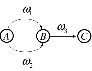
Trust propagation in OSNs was well-known, however, there is a lack of understanding about how to computationally model the process in practice. Trust propagation can be illustrated by a series topology, as shown in Fig. 1(a). In the figure, two edges are connected in series if they are incident to a vertex of degree $2$. Trust propagation means that if user $A_{i-1}$ trusts $A_{i}$ and $A_{i}$ trusts $A_{i+1}$, then $A_{i-1}$ can derive an indirect trust of $A_{i+1}$, even if $A_{i-1}$ did not interact with $A_{i+1}$ before.

Based on existing literature on trust propagation [16, 17, 18, 19], it is commonly agreed that the following assumptions hold.

• •

  A1: If $A$ trusts $B$, $B$ trusts $C$, then $A$ trusts $C$.

• •

  A2: If $A$ trusts $B$, $B$ does not trust $C$, then $A$ does not trust $C$.

• •

  A3: If $A$ trusts $B$, $B$ is uncertain about the trust of $C$, then $A$ is uncertain about $C$’s trust.

• •

  A4: If $A$ does not trust $B$, or $A$ is uncertain about $B$, then $A$ is uncertain about the trust of $C$.

It is worth mentioning that if $A$ does not trust or is uncertain about $B$, then $A$ is uncertain about $C$, and $B$’s opinion on $C$ cannot propagate to $A$. Based on the above-mentioned four assumptions, the trust propagation process can be modelled by the logic operation on two trust opinions.

Let’s denote $A$’s opinion on $B$ as

$$\omega_{AB}=\left<\alpha_{AB},\beta_{AB},\gamma_{AB}\right>,$$

and $B$’s opinion on $C$ as

$$\omega_{BC}=\left<\alpha_{BC},\beta_{BC},\gamma_{BC}\right>,$$

where $\{\alpha_{AB},\beta_{AB},\gamma_{AB}\}=\mathbf{D}_{AB}$ and $\{\alpha_{BC},\beta_{BC},\gamma_{BC}\}=\mathbf{D}_{BC}$ represent the observations made by $A$ and $B$, about $B$ and $C$, respectively. In this way, the expected probability that $C$ will behave as what $A$ expects will be

	$\displaystyle\iint(x=1|{{\bf{p}}_{AB}})f({{\bf{p}}_{AB}}|{{\bf{D}}_{AB}})\times$
	$\displaystyle f(x=1|{{\bf{p}}_{BC}})f({{\bf{p}}_{BC}}|{{\bf{D}}_{BC}})d({{\bf{p}}_{AB}})d({{\bf{p}}_{BC}}).$
			(3.4)

The equation makes sense because $A$ trusts $C$ if and only if $A$ trusts $B$ and $B$ trusts $C$, which is the assumption A1. In other words, the probability that $C$ will behave as what $A$ expects is equal to the probability that $C$ will behave as what $B$ expects, if $A$ trusts $B$. In the above equation, $f(x=1|\mathbf{p}_{AB})f(\mathbf{p}_{AB}|\mathbf{D}_{AB})$ gives the probability that $A$ trusts $B$, and $f(x=1|\mathbf{p}_{BC})f(\mathbf{p}_{BC}|\mathbf{D}_{BC})d(\mathbf{p}_{AB})$ is the probability that $B$ trusts $C$.

Because the probabilities that $A$ trusts $B$ and $B$ trusts $C$ are independent of each other, Eq. 3.4 can be rewritten as

	$\displaystyle\int f(x=1|\mathbf{p}_{AB})f(\mathbf{p}_{AB}|\mathbf{D}_{AB})d(\mathbf{p}_{AB})\times$
	$\displaystyle\int f(x=1|\mathbf{p}_{BC})f(\mathbf{p}_{BC}|\mathbf{D}_{BC})d(\mathbf{p}_{BC}).$		(3.5)

The two integrals in the equation are used to compute the expected probabilities that $A$ trusts $B$ and $B$ trusts $C$, respectively. According to Eq. 3.3, we know

			$\displaystyle\int f(x=1|\mathbf{p}_{AB})f(\mathbf{p}_{AB}|\mathbf{D}_{AB})d(\mathbf{p}_{AB})$
		$\displaystyle=$	$\displaystyle\frac{\alpha_{AB}}{\alpha_{AB}+\beta_{AB}+\gamma_{AB}},$

and

			$\displaystyle\int f(x=1|\mathbf{p}_{BC})f(\mathbf{p}_{BC}|\mathbf{D}_{BC})d(\mathbf{p}_{BC})$
		$\displaystyle=$	$\displaystyle\frac{\alpha_{BC}}{\alpha_{BC}+\beta_{BC}+\gamma_{BC}}.$

Inserting these two values into Eq. 3.5, we have the probability that $C$ will behave as what $A$ expects as

$$\frac{\alpha_{AB}\alpha_{BC}}{(\alpha_{AB}+\beta_{AB}+\gamma_{AB})(\alpha_{BC}+\beta_{BC}+\gamma_{BC})}.$$

(3.6)

According to assumption A2, the probability that $C$ will not behave as what $A$ expects is

	$\displaystyle\iint f(x=1|\mathbf{p}_{AB})f(\mathbf{p}_{AB}|\mathbf{D}_{AB})\times$
	$\displaystyle f(x=2|\mathbf{p}_{BC})f(\mathbf{p}_{BC}|\mathbf{D}_{BC})d(\mathbf{p}_{AB})d(\mathbf{p}_{BC}).$
			(3.7)

This is because $A$ does not trust $C$, if and only if $A$ trusts $B$ but $B$ does not trust $C$. Because these probabilities are independent, we have the expected probability that $A$ does not trust $C$ as

$$\frac{\alpha_{AB}\beta_{BC}}{(\alpha_{AB}+\beta_{AB}+\gamma_{AB})(\alpha_{BC}+\beta_{BC}+\gamma_{BC})}.$$

(3.8)

Finally, based on assumptions A3 and A4, the expected probability that $C$ will behave in an ambiguous way is

$$\begin{split}&\iint f(x=1|\mathbf{p}_{AB})f(\mathbf{p}_{AB}|\mathbf{D}_{AB})\times\\ &f(x=3|\mathbf{p}_{BC})f(\mathbf{p}_{BC}|\mathbf{D}_{BC})+\\ &f(x=2|\mathbf{p}_{AB})f(\mathbf{p}_{AB}|\mathbf{D}_{AB})+f(x=3|\mathbf{p}_{AB})f(\mathbf{p}_{AB}|\mathbf{D}_{AB})\\ &d(\mathbf{p}_{AB})d(\mathbf{p}_{BC}).\\ \end{split}$$

The expected probability can be rewritten as

$$\displaystyle\frac{\alpha_{AB}\gamma_{BC}+(\beta_{AB}+\gamma_{AB})(\alpha_{BC}+\beta_{BC}+\gamma_{BC})}{(\alpha_{AB}+\beta_{AB}+\gamma_{AB})(\alpha_{BC}+\beta_{BC}+\gamma_{BC})}.$$

(3.9)

The summation of Eqs. 3.4, 3.7 and 3.3 equals $1$. The three equations actually give the estimated probabilities that $C$ will behave as expected, not as expected, or in an ambiguous way, respectively. Putting these values back into the Categorical distribution

$$f(x|\mathbf{p}_{AC})=\prod_{i=1}^{3}p_{i}^{[x=i]},$$

(3.10)

where $\mathbf{p}_{AC}=(p_{1},p_{2},p_{3})$ and

	$\displaystyle{p_{1}}=\displaystyle\frac{{{\alpha_{AB}}{\alpha_{BC}}}}{{({\alpha_{AB}}+{\beta_{AB}}+{\gamma_{AB}})({\alpha_{BC}}+{\beta_{BC}}+{\gamma_{BC}})}}$
	$\displaystyle{p_{2}}=\displaystyle\frac{{{\alpha_{AB}}{\beta_{BC}}}}{{({\alpha_{AB}}+{\beta_{AB}}+{\gamma_{AB}})({\alpha_{BC}}+{\beta_{BC}}+{\gamma_{BC}})}},$
	$\displaystyle{p_{3}}=\displaystyle\frac{{({\beta_{AB}}+{\gamma_{AB}})({\alpha_{BC}}+{\beta_{BC}}+{\gamma_{BC}})+{\alpha_{AB}}{\gamma_{BC}}}}{{({\alpha_{AB}}+{\beta_{AB}}+{\gamma_{AB}})({\alpha_{BC}}+{\beta_{BC}}+{\gamma_{BC}})}}$
			(3.11)

we can compute the probability that $X$ is trustworthy.

From the above description, we know the Categorical distribution is in fact derived from $B$’s opinion on $C$. Let’s assume $B$ made the observations $\mathbf{x}=\{x_{1},x_{2},\cdots,x_{n}\}$ on $C$. Then, we know $\alpha_{BC},\beta_{BC},\gamma_{BC}$ equal to the numbers of observations where $x=1,x=2,x=3$, respectively. Clearly, the observations $B$ made about $C$ do not reflect $A$’s opinion on $C$. As trust propagates among users, $A$ could derive an indirect opinion from $B$’s observations of $C$. One may ask the question that if $A$ was provided with the $n$ observations, how many of them will be considered positive, negative, and uncertain, from $A$’s perspective. That implies$A$ needs to reuse $B$’s observations on $C$ to derive its own opinion on $C$. For each $x_{j}\in\mathbf{x}$ where $j=1,2,\cdots,n$, we know $x_{j}$ is observed, given the underlying categorical distribution shown in Eq. 3.10. In other words, $\mathbf{x}$ follows the multinomial distribution with parameters $(n,\mathbf{p}_{AC})$. From the multinomial distribution, we can recompute the probability that $C$ is trustworthy, by re-categorizing the observations $\mathbf{x}$. We know the following re-categorization will occur with the highest probability.

	$\displaystyle\alpha_{AC}$	$\displaystyle=$	$\displaystyle p_{1}(\alpha_{BC}+\beta_{BC}+\gamma_{BC})$
		$\displaystyle=$	$\displaystyle\displaystyle\frac{\alpha_{AB}\alpha_{BC}}{(\alpha_{AB}+\beta_{AB}+\gamma_{AB})},$
	$\displaystyle\beta_{AC}$	$\displaystyle=$	$\displaystyle p_{2}(\alpha_{BC}+\beta_{BC}+\gamma_{BC})$
		$\displaystyle=$	$\displaystyle\displaystyle\frac{\alpha_{AB}\beta_{BC}}{(\alpha_{AB}+\beta_{AB}+\gamma_{AB})},$
	$\displaystyle\gamma_{AC}$	$\displaystyle=$	$\displaystyle p_{3}(\alpha_{BC}+\beta_{BC}+\gamma_{BC}),$
		$\displaystyle=$	$\displaystyle\displaystyle\frac{(\beta_{AB}+\gamma_{AB})(\alpha_{BC}+\beta_{BC}+\gamma_{BC})+\alpha_{AB}\gamma_{BC}}{(\alpha_{AB}+\beta_{AB}+\gamma_{AB})}.$

Therefore, we use $\omega_{AC}=\left<\alpha_{AC},\beta_{AC},\gamma_{AC}\right>$ to represent $A$’s opinion about $C$’s trust. Note that the opinion $\omega_{AC}$ is generated by distorting positive and negative evidence in $\omega_{BC}$ to uncertain evidence. That also means the total amount of evidence does not change in trust propagation.

$\displaystyle{\alpha_{AC}}+{\beta_{AC}}+{\gamma_{AC}}={\alpha_{BC}}+{\beta_{BC}}+{\gamma_{BC}}.$

(3.13)

Based on the previous analysis, we formally define the discounting operation in 3VSL as follows.

Opinion $\omega_{BC}$ being discounted can be viewed as the certain evidence in $\omega_{BC}$ are distorted by opinion $\omega_{AB}$, and then transferred into the uncertainty space of $\omega_{AC}$. Because the total amount of evidence in opinion $\omega_{AC}=\mathchar 257\relax(\omega_{AB},\omega_{BC})$ is the same as $\omega_{BC}$’s, we conclude the resulting opinion of discounting operation shares exactly the same evidence space as the original opinion.

Based on the definition of discounting operation, it offers two interesting properties: decay and associative properties.

In other words, by applying the discounting operation, the uncertainty in trust (or in the resulting opinion) increases. This property implies that the more trust propagates among users in an OSN, the more uncertain the resulting opinion.

However, the discounting operation is not commutative, i.e., $\mathchar 257\relax(\omega_{AB},\omega_{BC})\neq\mathchar 257\relax(\omega_{BC},\omega_{AB})$. Given a series topology where opinions are ordered as $\omega_{A_{1}A_{2}},\omega_{A_{2},A_{3}},\cdots,$ $\omega_{A_{n-1}A_{n}}$, the final opinion can be calculated as $\mathchar 257\relax(\mathchar 257\relax(\mathchar 257\relax(\omega_{A_{1}A_{2}},\omega_{A_{2}A_{3}}),\cdots),\omega_{A_{n-1}A_{n}})$. As the discounting operation is associative, it can be simplified as $\mathchar 257\relax(\omega_{{A_{1}A_{2}}},\omega_{A_{2}A_{3}},\cdots\omega_{A_{n-1}A_{n}})$.

According to previous works [16, 17, 18], trust opinions can be fused into a consensus one by aggregating the evidence from each opinion. We will use the parallel topology shown in Fig. 2 to explain how the combining operation works.

Let $\omega_{{A_{1}}{B_{1}}}=\left<\alpha_{{A_{1}}{B_{1}}},\beta_{{A_{1}}{B_{1}}},\gamma_{{A_{1}}{B_{1}}}\right>$ and $\omega_{{A_{2}}{B_{2}}}=\left<\alpha_{{A_{2}}{B_{2}}},\beta_{{A_{2}}{B_{2}}},\gamma_{{A_{2}}{B_{2}}}\right>$ be $A$’s two indirect/direct opinions on $B$. We use $\{\alpha_{{A_{1}}{B_{1}}},\beta_{{A_{1}}{B_{1}}},\gamma_{{A_{1}}{B_{1}}}\}=\mathbf{D}_{{A_{1}}{B_{1}}}$ and $\{\alpha_{{A_{2}}{B_{2}}},\beta_{{A_{2}}{B_{2}}},\gamma_{{A_{2}}{B_{2}}}\}=\mathbf{D}_{{A_{2}}{B_{2}}}$ to represent the two sets of observations $A$ made on $B$. According to the definition of an opinion, the expected probability that $B$ will behave as what $A$ expects can be computed from the following DC distribution.

$$\int{f(x=1|{{\bf{p}}_{AB}})f({{\bf{p}}_{AB}}|{{\bf{D}}_{{A_{1}}{B_{1}}}},{{\bf{D}}_{{A_{2}}{B_{2}}}})d({{\bf{p}}_{AB}})},$$

(3.15)

The intuition of Eq. 3.15 can be explained as follows. $A$ first infers the parameters ${\bf{p}}_{AB}$ by aggregating the observations ${\bf{D}}_{{A_{1}}{B_{1}}}$ and ${\bf{D}}_{{A_{2}}{B_{2}}}$, i.e., the posterior pdf of ${\bf{p}}_{AB}$ becomes

$$f({{\bf{p}}_{AB}}|{{\bf{D}}_{{A_{1}}{B_{1}}}},{{\bf{D}}_{{A_{2}}{B_{2}}}}).$$

(3.16)

Then, based on the inferred parameters ${\bf{p}}_{AB}$, the probability that $B$ will behave as what $A$ expects can be computed from $f(x=1|{{\bf{p}}_{AB}})$. Considering all possible values of ${\bf{p}}_{AB}$, we can obtain the Eq. 3.15.

Now, we will give the analytic form of Eq. 3.16 as follows. $A$ first forms his opinion on $B$ from ${{\bf{D}}_{{A_{1}}{B_{1}}}}$. As such, the pdf of ${{\bf{p}}_{{A}{B}}}$ is obtained. Then, $A$ adjusts the estimate for ${{\bf{p}}_{{A}{B}}}$ based on another set of evidence ${{\bf{D}}_{{A_{2}}{B_{2}}}}$. As a matter of fact, Eq. 3.16 can be regarded as the distribution of ${{\bf{p}}_{{A}{B}}}$ based on (1) the posterior evidence in ${{\bf{D}}_{{A_{2}}{B_{2}}}}$ and (2) the prior parameters ${{\bf{p}}_{{A_{1}}{B_{1}}}}$ estimated from ${{\bf{D}}_{{A_{1}}{B_{1}}}}$. According to Bayesian inference, it can be expressed as follows.

			$\displaystyle f({{\bf{p}}_{AB}}|{{\bf{D}}_{{A_{1}}{B_{1}}}},{{\bf{D}}_{{A_{2}}{B_{2}}}})$		(3.17)
		$\displaystyle=$	$\displaystyle\displaystyle\frac{{f({{\bf{D}}_{{A_{2}}{B_{2}}}}|{\bf{p}}_{{A_{1}}{B_{1}}})f({\bf{p}}_{{A_{1}}{B_{1}}})}}{{f({{\bf{D}}_{{A_{2}}{B_{2}}}})}}$
		$\displaystyle=$	$\displaystyle\displaystyle\frac{{f({{\bf{D}}_{{A_{2}}{B_{2}}}}|{\bf{p}}_{{A_{1}}{B_{1}}})f({\bf{p}}_{{A_{1}}{B_{1}}})}}{{\displaystyle\int{f({{\bf{D}}_{{A_{2}}{B_{2}}}}|{\bf{p}}_{{A_{1}}{B_{1}}})f({\bf{p}}_{{A_{1}}{B_{1}}})}d{\bf{p}}_{{A_{1}}{B_{1}}}}}.$

In the equation, ${\bf{p}}_{{A_{1}}{B_{1}}}$ is derived from ${{\bf{D}}_{{A_{1}}{B_{1}}}}$ that follows Dirichlet distribution, so its pdf can be computed as follows.

			$\displaystyle f({\bf{p}}_{{A_{1}}{B_{1}}})$
		$\displaystyle=$	$\displaystyle\frac{{\mathchar 256\relax({\alpha_{{A_{1}}{B_{1}}}}+{\beta_{{A_{1}}{B_{1}}}}+{\gamma_{{A_{1}}{B_{1}}}})}}{{\mathchar 256\relax({\alpha_{{A_{1}}{B_{1}}}})\mathchar 256\relax({\beta_{{A_{1}}{B_{1}}}})\mathchar 256\relax({\gamma_{{A_{1}}{B_{1}}}})}}\times$
			$\displaystyle({p_{1}})^{{\alpha_{{A_{1}}{B_{1}}}}-1}{({p_{2}})^{{\beta_{{A_{1}}{B_{1}}}}-1}}({p_{3}})^{{\gamma_{{A_{1}}{B_{1}}}}-1}.$

On the other hand, because ${{\bf{D}}_{{A_{2}}{B_{2}}}}$ follows the multinomial distribution, derived from ${\bf{p}}_{{A_{1}}{B_{1}}}$, its pdf can be expressed as

			$\displaystyle f({{\bf{D}}_{{A_{2}}{B_{2}}}}|{\bf{p}}_{{A_{1}}{B_{1}}})$
		$\displaystyle=$	$\displaystyle\frac{{\mathchar 256\relax({\alpha_{{A_{2}}{B_{2}}}}+{\beta_{{A_{2}}{B_{2}}}}+{\gamma_{{A_{2}}{B_{2}}}}+1)}}{{\mathchar 256\relax({\alpha_{{A_{2}}{B_{2}}}}+1)\mathchar 256\relax({\beta_{{A_{2}}{B_{2}}}}+1)\mathchar 256\relax({\gamma_{{A_{2}}{B_{2}}}}+1)}}\times$
			$\displaystyle{({p_{1}})^{{\alpha_{{A_{2}}{B_{2}}}}}}{({p_{2}})^{{\beta_{{A_{2}}{B_{2}}}}}}{({p_{3}})^{{\gamma_{{A_{2}}{B_{2}}}}}}.$

Substituting Eq.  and Eq.  for $f({\bf{p}}_{{A_{1}}{B_{1}}})$ and $f({{\bf{D}}_{{A_{2}}{B_{2}}}}|{\bf{p}}_{{A_{1}}{B_{1}}})$ in Eq. 3.17, the analytic form of Eq. 3.16 will be

			$\displaystyle f({{\bf{p}}_{AB}}|{{\bf{D}}_{{A_{1}}{B_{1}}}},{{\bf{D}}_{{A_{2}}{B_{2}}}})$
		$\displaystyle=$	$\displaystyle\frac{{\mathchar 256\relax({\alpha_{AB}}+{\beta_{AB}}+{\gamma_{AB}})}}{{\mathchar 256\relax({\alpha_{AB}})\mathchar 256\relax({\beta_{AB}})\mathchar 256\relax({\gamma_{AB}})}}\times$
			$\displaystyle{({p_{1}})^{{\alpha_{AB}}-1}}{({p_{2}})^{{\beta_{AB}}-1}}{({p_{3}})^{{\gamma_{AB}}-1}},$

where

	$\displaystyle\alpha_{AB}$	$\displaystyle=$	$\displaystyle\alpha_{{A_{1}}{B_{1}}}+\alpha_{{A_{2}}{B_{2}}},$
	$\displaystyle\beta_{AB}$	$\displaystyle=$	$\displaystyle\beta_{{A_{1}}{B_{1}}}+\beta_{{A_{2}}{B_{2}}},$
	$\displaystyle\gamma_{AB}$	$\displaystyle=$	$\displaystyle\gamma_{{A_{1}}{B_{1}}}+\gamma_{{A_{2}}{B_{2}}}.$

Obviously, Eq.  can be considered the most likely pdf of the following Dirichlet distribution.

$$Dir({\alpha_{{A_{1}}{B_{1}}}}+{\alpha_{{A_{2}}{B_{2}}}},{\beta_{{A_{1}}{B_{1}}}}+{\beta_{{A_{2}}{B_{2}}}},{\gamma_{{A_{1}}{B_{1}}}}+{\gamma_{{A_{2}}{B_{2}}}}).$$

Then, the equation

$\displaystyle\int{f(x|{{\bf{p}}_{AB}})f({{\bf{p}}_{AB}}|{{\bf{D}}_{{A_{1}}{B_{1}}}},{{\bf{D}}_{{A_{2}}{B_{2}}}})d({{\bf{p}}_{AB}})}$

can be regarded as a DC distribution upon observations $\{{\alpha_{{A_{1}}{B_{1}}}}+{\alpha_{{A_{2}}{B_{2}}}},{\beta_{{A_{1}}{B_{1}}}}+{\beta_{{A_{2}}{B_{2}}}},{\gamma_{{A_{1}}{B_{1}}}}+{\gamma_{{A_{2}}{B_{2}}}}\}$. The above description essentially reflects the important property of DC distribution: two DC distributions can be combined, by adding up the corresponding controlling hyper-parameters, to yield a new DC distribution.

References

- [1] G. Liu, Q. Yang, H. Wang, and A. X. Liu. Three-valued subjective logic: A model for trust assessment in online social networks. IEEE Transactions on Dependable and Secure Computing, pages 1–1, 2019.
- [2] Anirban Basu, Jaideep Vaidya, Juan Camilo Corena, Shinsaku Kiyomoto, Stephen Marsh, Guibing Guo, Jie Zhang, and Yutaka Miyake. Opinions of people: Factoring in privacy and trust. SIGAPP Appl. Comput. Rev., 14(3):7–21, September 2014.
- [3] Paul Resnick, Ko Kuwabara, Richard Zeckhauser, and Eric Friedman. Reputation systems. Communications of the ACM, 43(12):45–48, 2000.
- [4] De-Nian Yang, Hui-Ju Hung, Wang-Chien Lee, and Wei Chen. Maximizing acceptance probability for active friending in online social networks. In 19th ACM SIGKDD, pages 713–721, 2013.
- [5] Dapeng Wu, Junjie Yan, Honggang Wang, Dalei Wu, and Ruyan Wang. Social attribute aware incentive mechanism for device-to-device video distribution. IEEE Transactions on Multimedia, 19(8):1908–1920, 2017.
- [6] T. Cheng, G. Liu, Q. Yang, and J. Sun. Trust assessment in vehicular social network based on three-valued subjective logic. IEEE Transactions on Multimedia, 21(3):652–663, March 2019.
- [7] G. Liu, Q. Chen, Q. Yang, B. Zhu, H. Wang, and W. Wang. Opinionwalk: An efficient solution to massive trust assessment in online social networks. In IEEE INFOCOM 2017 - IEEE Conference on Computer Communications, pages 1–9, May 2017.
- [8] Guangchi Liu, Qing Yang, Honggang Wang, Xiaodong Lin, and M.P. Wittie. Assessment of multi-hop interpersonal trust in social networks by three-valued subjective logic. In INFOCOM, 2014 Proceedings IEEE, pages 1698–1706, April 2014.
- [9] X. Niu, G. Liu, and Q. Yang. Trustworthy website detection based on social hyperlink network analysis. IEEE Transactions on Network Science and Engineering, pages 1–1, 2018.
- [10] Denise M Rousseau, Sim B Sitkin, Ronald S Burt, and Colin Camerer. Not so different after all: A cross-discipline view of trust. Academy of management review, 23(3):393–404, 1998.
- [11] D Harrison McKnight, Vivek Choudhury, and Charles Kacmar. Developing and validating trust measures for e-commerce: An integrative typology. Information systems research, 13(3):334–359, 2002.
- [12] Rino Falcone and Cristiano Castelfranchi. Social trust: A cognitive approach. In Trust and deception in virtual societies, pages 55–90. Springer, 2001.
- [13] Audun Jøsang. A logic for uncertain probabilities. International Journal of Uncertainty, Fuzziness and Knowledge-Based Systems, 9(03):279–311, 2001.
- [14] Guangchi Liu, Qing Yang, Honggang Wang, Shaoen Wu, and M. P. Wittie. Uncovering the mystery of trust in an online social network. In 2015 IEEE Conference on Communications and Network Security (CNS), pages 488–496, Sept 2015.
- [15] Stephen Tu. The dirichlet-multinomial and dirichlet-categorical models for bayesian inference. Computer Science Division, UC Berkeley, Tech. Rep.[Online]. Available: http://www. cs. berkeley. edu/ stephentu/writeups/dirichlet-conjugate-prior. pdf, 2014.
- [16] R. Guha, Ravi Kumar, Prabhakar Raghavan, and Andrew Tomkins. Propagation of trust and distrust. In Proceedings of the 13th International Conference on World Wide Web, WWW ’04, pages 403–412, New York, NY, USA, 2004. ACM.
- [17] Christian Borgs, Jennifer Chayes, Adam Tauman Kalai, Azarakhsh Malekian, and Moshe Tennenholtz. A Novel Approach to Propagating Distrust, pages 87–105. Springer Berlin Heidelberg, Berlin, Heidelberg, 2010.
- [18] Cai-Nicolas Ziegler and Georg Lausen. Propagation models for trust and distrust in social networks. Information Systems Frontiers, 7(4):337–358, 2005.
- [19] Ramanthan Guha, Ravi Kumar, Prabhakar Raghavan, and Andrew Tomkins. Propagation of trust and distrust. In Proceedings of the 13th international conference on World Wide Web, pages 403–412. ACM, 2004.
- [20] Yonghong Wang and Munindar P. Singh. Formal trust model for multiagent systems. In Proceedings of the 20th International Joint Conference on Artifical Intelligence, IJCAI’07, pages 1551–1556, San Francisco, CA, USA, 2007. Morgan Kaufmann Publishers Inc.
- [21] Andreas Jakoby, Maciej Liskiewicz, and Rüdiger Reischuk. Space efficient algorithms for series-parallel graphs. In STACS 2001, pages 339–352. Springer, 2001.
- [22] Chung-Wei Hang, Yonghong Wang, and Munindar P. Singh. Operators for propagating trust and their evaluation in social networks. In Proceedings of The 8th International Conference on Autonomous Agents and Multiagent Systems - Volume 2, AAMAS ’09, pages 1025–1032, Richland, SC, 2009. International Foundation for Autonomous Agents and Multiagent Systems.
- [23] Chung-Wei Hang and Munindar P Singh. Trust-based recommendation based on graph similarity. In Proceedings of the 13th International Workshop on Trust in Agent Societies (TRUST). Toronto, Canada, 2010.
- [24] Chung-Wei Hang, Yonghong Wang, and Munindar P. Singh. Operators for propagating trust and their evaluation in social networks. In Proceedings of The 8th International Conference on Autonomous Agents and Multiagent Systems - Volume 2, AAMAS ’09, pages 1025–1032, Richland, SC, 2009. International Foundation for Autonomous Agents and Multiagent Systems.
- [25] f1 score. http://scikit-learn.org/stable/modules/generated/sklearn.metrics.f1_score.
- [26] Daniel A Powers and Yu Xie. Statistical methods for categorical data analysis. Emerald Group Publishing, 2008.
- [27] Jennifer Ann Golbeck. Computing and Applying Trust in Web-based Social Networks. PhD thesis, College Park, MD, USA, 2005. AAI3178583.
- [28] Zoltán Gyöngyi, Hector Garcia-Molina, and Jan Pedersen. Combating web spam with trustrank. In Proceedings of the Thirtieth International Conference on Very Large Data Bases - Volume 30, VLDB ’04, pages 576–587. VLDB Endowment, 2004.
- [29] Sepandar D. Kamvar, Mario T. Schlosser, and Hector Garcia-Molina. The eigentrust algorithm for reputation management in p2p networks. In Proceedings of the 12th International Conference on World Wide Web, WWW ’03, pages 640–651, New York, NY, USA, 2003. ACM.
- [30] David Gefen, Elena Karahanna, and Detmar W. Straub. Trust and tam in online shopping: An integrated model. MIS Q., 27(1):51–90, March 2003.
- [31] Diego Gambetta. Trust: Making and Breaking Cooperative Relations, volume 52. Blackwell, 1988.
- [32] Patricia M Doney and Joseph P Cannon. An examination of the nature of trust in buyer-seller relationships. the Journal of Marketing, pages 35–51, 1997.
- [33] Christine Moorman, Gerald Zaltman, and Rohit Deshpande. Relationships between providers and users of market research: The dynamics of trust. Journal of marketing research, 29(3):314–328, 1992.
- [34] Shankar Ganesan. Determinants of long-term orientation in buyer-seller relationships. the Journal of Marketing, pages 1–19, 1994.
- [35] Sirkka L Jarvenpaa, Noam Tractinsky, and Lauri Saarinen. Consumer trust in an internet store: a cross-cultural validation. Journal of Computer-Mediated Communication, 5(2):0–0, 1999.
- [36] Wei Wei, Fengyuan Xu, C.C. Tan, and Qun Li. Sybildefender: Defend against sybil attacks in large social networks. In INFOCOM, 2012 Proceedings IEEE, pages 1951–1959, March 2012.
- [37] George Danezis and Prateek Mittal. SybilInfer: Detecting sybil nodes using social networks. In Proceedings of the Network and Distributed System Security Symposium, NDSS 2009, San Diego, California, USA, 8th February - 11th February 2009, 2009.
- [38] Haifeng Yu, Michael Kaminsky, Phillip B. Gibbons, and Abraham D. Flaxman. Sybilguard: Defending against sybil attacks via social networks. IEEE/ACM Trans. Netw., 16(3):576–589, June 2008.
- [39] Haifeng Yu, P.B. Gibbons, M. Kaminsky, and Feng Xiao. SybilLimit: A near-optimal social network defense against sybil attacks. Networking, IEEE/ACM Transactions on, 18(3):885–898, June 2010.
- [40] T. DuBois, J. Golbeck, and A. Srinivasan. Rigorous probabilistic trust-inference with applications to clustering. In Web Intelligence and Intelligent Agent Technologies, 2009. WI-IAT ’09. IEEE/WIC/ACM International Joint Conferences on, volume 1, pages 655–658, Sept 2009.
- [41] Yanjun Zuo, Wen-chen Hu, and Timothy O’Keefe. Trust computing for social networking. In Information Technology: New Generations, 2009. ITNG’09. Sixth International Conference on, pages 1534–1539. IEEE, 2009.
- [42] Jennifer Ann Golbeck. Computing and applying trust in web-based social networks. 2005.
- [43] Yu Zhang, Huajun Chen, and Zhaohui Wu. A social network-based trust model for the semantic web. In LaurenceT. Yang, Hai Jin, Jianhua Ma, and Theo Ungerer, editors, Autonomic and Trusted Computing, volume 4158 of Lecture Notes in Computer Science, pages 183–192. Springer Berlin Heidelberg, 2006.
- [44] Lawrence Page, Sergey Brin, Rajeev Motwani, and Terry Winograd. The pagerank citation ranking: Bringing order to the web. Technical report, Stanford InfoLab, 1999.
- [45] Zoran Despotovic and Karl Aberer. Probabilistic prediction of peers’ performance in {P2P} networks. Engineering Applications of Artificial Intelligence, 18(7):771 – 780, 2005.
- [46] WT Teacy, Michael Luck, Alex Rogers, and Nicholas R Jennings. An efficient and versatile approach to trust and reputation using hierarchical Bayesian modelling. Artificial Intelligence, 193(0):149 – 185, 2012.
- [47] Ehab ElSalamouny, Vladimiro Sassone, and Mogens Nielsen. HMM-based trust model. In Formal Aspects in Security and Trust, pages 21–35. Springer, 2010.
- [48] Xin Liu and Anwitaman Datta. Modeling context aware dynamic trust using hidden markov model. In AAAI, 2012.
- [49] George Vogiatzis, Ian MacGillivray, and Maria Chli. A probabilistic model for trust and reputation. In Proceedings of the 9th International Conference on Autonomous Agents and Multiagent Systems: volume 1-Volume 1, pages 225–232. International Foundation for Autonomous Agents and Multiagent Systems, 2010.
- [50] Carol J Fung, Jie Zhang, Issam Aib, and Raouf Boutaba. Dirichlet-based trust management for effective collaborative intrusion detection networks. Network and Service Management, IEEE Transactions on, 8(2):79–91, 2011.
- [51] Audun Jøsang and Simon Pope. Semantic constraints for trust transitivity. In Proceedings of the 2Nd Asia-Pacific Conference on Conceptual Modelling - Volume 43, APCCM ’05, pages 59–68, Darlinghurst, Australia, Australia, 2005. Australian Computer Society, Inc.
- [52] A. Josang and T. Bhuiyan. Optimal trust network analysis with subjective logic. In Emerging Security Information, Systems and Technologies, 2008. SECURWARE ’08. Second International Conference on, pages 179–184, Aug 2008.
- [53] Yonghong Wang and Munindar P Singh. Trust representation and aggregation in a distributed agent system. In AAAI, volume 6, pages 1425–1430, 2006.
- [54] Yonghong Wang, Chung-Wei Hang, and Munindar P. Singh. A probabilistic approach for maintaining trust based on evidence. J. Artif. Int. Res., 40(1):221–267, January 2011.
- [55] Yonghong Wang and Munindar P. Singh. Evidence-based trust: A mathematical model geared for multiagent systems. ACM Trans. Auton. Adapt. Syst., 5(4):14:1–14:28, November 2010.
- [56] Ugur Kuter and Jennifer Golbeck. Using probabilistic confidence models for trust inference in web-based social networks. ACM Trans. Internet Technol., 10(2):8:1–8:23, June 2010.
- [57] Audun Jøsang. The consensus operator for combining beliefs. Artificial Intelligence, 141(1):157–170, 2002.
- [58] Audun Jøsang, Stephen Marsh, and Simon Pope. Exploring different types of trust propagation. In Trust management, pages 179–192. Springer, 2006.
- [59] Audun Jøsang and David McAnally. Multiplication and comultiplication of beliefs. International Journal of Approximate Reasoning, 38(1):19–51, 2005.
- [60] Audun Josang. Conditional reasoning with subjective logic. Journal of Multiple-Valued Logic and Soft Computing, 15(1):5–38, 2008.
- [61] Audun Jøsang. Probabilistic logic under uncertainty. In Proceedings of the thirteenth Australasian symposium on Theory of computing-Volume 65, pages 101–110. Australian Computer Society, Inc., 2007.
- [62] M. Assefi, E. Behravesh, G. Liu, and A. P. Tafti. Big data machine learning using apache spark mllib. In 2017 IEEE International Conference on Big Data (Big Data), pages 3492–3498, Dec 2017.
- [63] A. Mohaisen, Huy Tran, A. Chandra, and Yongdae Kim. Trustworthy distributed computing on social networks. Services Computing, IEEE Transactions on, 7(3):333–345, July 2014.
- [64] Yang Zhou, Yan Huang, Joseph McGlynn, and Alexander Han. Who will you share a ride with: Factors that influence trust of potential rideshare partners. arXiv preprint arXiv:1707.04284, 2017.
- [65] Y. Zhou and Y. Huang. Deepmove: Learning place representations through large scale movement data. In 2018 IEEE International Conference on Big Data (Big Data), pages 2403–2412, Dec 2018.
- [66] Y. Zhou and Y. Huang. Context aware flow prediction of bike sharing systems. In 2018 IEEE International Conference on Big Data (Big Data), pages 2393–2402, Dec 2018.
- [67] Mehdi Assefi, Guangchi Liu, Mike P Wittit, and Clemente Izurieta. Measuring the impact of network performance on cloud-based speech recognition applications. International Journal of Computer Applications-IJCA, 23:19–28, 2016.
- [68] Francisco Moyano, Carmen Fernandez-Gago, and Javier Lopez. A framework for enabling trust requirements in social cloud applications. Requirements Engineering, 18:321–341, Nov 2013 2013.
- [69] Mehdi Assefi, Guangchi Liu, Mike P Wittie, and Clemente Izurieta. An experimental evaluation of apple siri and google speech recognition. Proccedings of the 2015 ISCA SEDE, pages 1–6, 2015.
- [70] Roberto Di Pietro, Flavio Lombardi, Fabio Martinelli, and Daniele Sgandurra. Anticheetah: Trustworthy computing in an outsourced (cheating) environment. Future Generation Computer Systems, 48(0):28 – 38, 2015. Special Section: Business and Industry Specific Cloud.
- [71] Runfang Zhou and Kai Hwang. Powertrust: A robust and scalable reputation system for trusted peer-to-peer computing. Parallel and Distributed Systems, IEEE Transactions on, 18(4):460–473, April 2007.
- [72] Li Xiong and Ling Liu. Peertrust: supporting reputation-based trust for peer-to-peer electronic communities. Knowledge and Data Engineering, IEEE Transactions on, 16(7):843–857, July 2004.
- [73] Matthew Richardson, Rakesh Agrawal, and Pedro Domingos. Trust management for the semantic web. In Dieter Fensel, Katia Sycara, and John Mylopoulos, editors, The Semantic Web - ISWC 2003, volume 2870 of Lecture Notes in Computer Science, pages 351–368. Springer Berlin Heidelberg, 2003.
- [74] Jennifer Golbeck, Bijan Parsia, and James Hendler. Trust networks on the semantic web. In Matthias Klusch, Andrea Omicini, Sascha Ossowski, and Heimo Laamanen, editors, Cooperative Information Agents VII, volume 2782 of Lecture Notes in Computer Science, pages 238–249. Springer Berlin Heidelberg, 2003.
- [75] Donovan Artz and Yolanda Gil. A survey of trust in computer science and the semantic web. Web Semantics: Science, Services and Agents on the World Wide Web, 5(2):58 – 71, 2007. Software Engineering and the Semantic Web.
- [76] P. Massa and C. Hayes. Page-rerank: using trusted links to re-rank authority. In Web Intelligence, 2005. Proceedings. The 2005 IEEE/WIC/ACM International Conference on, pages 614–617, Sept 2005.
- [77] Jon M. Kleinberg. Authoritative sources in a hyperlinked environment. J. ACM, 46(5):604–632, September 1999.
- [78] Li Ding, Pranam Kolari, Tim Finin, Anupam Joshi, Yun Peng, and Yelena Yesha. On homeland security and the semantic web: A provenance and trust aware inference framework. In In AAAI Spring Symposium on AI Technologies for Homeland Security, pages 21–23. AAAI Press, 2005.
- [79] Li Ding, Lina Zhou, and Timothy Finin. Trust based knowledge outsourcing for semantic web agents. In Proceedings of the 2003 IEEE/WIC International Conference on Web Intelligence, WI ’03, pages 379–, Washington, DC, USA, 2003. IEEE Computer Society.
- [80] Christian Bizer, Richard Cyganiak, Tobias Gauss, and Oliver Maresch. O.: The triql.p browser: Filtering information using context-, content- and rating-based trust policies. In Proceedings of the Semantic Web and Policy Workshop, held in conjunction with the 4th International Semantic Web Conference, 7 November, 2005, pages 12–20, 2005.
- [81] Doug Downey, Oren Etzioni, and Stephen Soderland. A probabilistic model of redundancy in information extraction. In Proceedings of the 19th International Joint Conference on Artificial Intelligence, IJCAI’05, pages 1034–1041, San Francisco, CA, USA, 2005. Morgan Kaufmann Publishers Inc.
- [82] Charles L. A. Clarke, Gordon V. Cormack, and Thomas R. Lynam. Exploiting redundancy in question answering. In Proceedings of the 24th Annual International ACM SIGIR Conference on Research and Development in Information Retrieval, SIGIR ’01, pages 358–365, New York, NY, USA, 2001. ACM.
- [83] Jennifer Golbeck. Trust and nuanced profile similarity in online social networks. ACM Trans. Web, 3(4):12:1–12:33, September 2009.
- [84] Xiaolan Zhu and Susan Gauch. Incorporating quality metrics in centralized/distributed information retrieval on the world wide web. In Proceedings of the 23rd Annual International ACM SIGIR Conference on Research and Development in Information Retrieval, SIGIR ’00, pages 288–295, New York, NY, USA, 2000. ACM.
- [85] Ellen Riloff, Janyce Wiebe, and William Phillips. Exploiting subjectivity classification to improve information extraction. In Proceedings of the 20th National Conference on Artificial Intelligence - Volume 3, AAAI’05, pages 1106–1111. AAAI Press, 2005.
- [86] Veselin Stoyanov, Claire Cardie, and Janyce Wiebe. Multi-perspective question answering using the opqa corpus. In Proceedings of the Conference on Human Language Technology and Empirical Methods in Natural Language Processing, HLT ’05, pages 923–930, Stroudsburg, PA, USA, 2005. Association for Computational Linguistics.
- [87] Yolanda Gil and Varun Ratnakar. Trusting information sources one citizen at a time. In Proceedings of the First International Semantic Web Conference on The Semantic Web, ISWC ’02, pages 162–176, London, UK, UK, 2002. Springer-Verlag.
- [88] Guangchi Liu and Guoliang Yao. E-mac: An event-driven data aggregation mac protocol for wireless sensor networks. In 2012 IEEE Consumer Communications and Networking Conference (CCNC), pages 941–946, Jan 2012.
- [89] X. Zhang, G. Liu, Q. Tian, and Z. Li. Mlmac: Multi-channel low-latency mac protocol for industrial wireless sensor networks. In 2011 International Conference on Internet of Things and 4th International Conference on Cyber, Physical and Social Computing, pages 338–342, Oct 2011.
- [90] Y. Zhang, X. Shen, Q. Yang, C. Qian, and G. Liu. Infusion auxiliary service system based on zigbee wireless network. IEEE Access, 6:12718–12726, 2018.
- [91] G. Liu and G. Yao. Srmac: Staggered routing-enhanced mac protocol for wireless sensor networks. In 2011 7th International Conference on Wireless Communications, Networking and Mobile Computing, pages 1–6, Sep. 2011.
- [92] Yu Liu, Zhong Yang, Xiaoyong Yan, Guangchi Liu, and Bo Hu. A novel multi-hop algorithm for wireless network with unevenly distributed nodes. Computers, Materials & Continua, 58(1):79–100, 2019.
- [93] Qi Chen, Ye Liu, Guangchi Liu, Qing Yang, Xianming Shi, Hongwei Gao, Lu Su, and Quanlong Li. Harvest energy from the water: A self-sustained wireless water quality sensing system. ACM Trans. Embed. Comput. Syst., 17(1):3:1–3:24, September 2017.
- [94] Y. Liu, Q. Chen, G. Liu, H. Liu, and Q. Yang. Ecosense: A hardware approach to on-demand sensing in the internet of things. IEEE Communications Magazine, 54(12):37–43, December 2016.
- [95] H. Gao, Q. Chen, and Q. Yang. Power management system for microbial fuel cell powered water quality monitoring system. In 2015 IEEE 16th Workshop on Control and Modeling for Power Electronics (COMPEL), pages 1–6, July 2015.
- [96] Y. Liu, Qi Chen, Hao Liu, Chen Hu, and Qing Yang. A non destructive interference based receiver-initiated mac protocol for wireless sensor networks. In 2016 13th IEEE Annual Consumer Communications Networking Conference (CCNC), pages 1030–1035, Jan 2016.
- [97] Qi Chen and Qing Yang. Understanding relative network delay inmicro-energy harvesting wireless networks. arXiv preprint arXiv:1908.07334, 2019.
- [98] Xiaoyan Hong, Dijiang Huang, Mario Gerla, and Zhen Cao. Sat: Situation-aware trust architecture for vehicular networks. In Proceedings of the 3rd International Workshop on Mobility in the Evolving Internet Architecture, MobiArch ’08, pages 31–36, 2008.
- [99] J. Hochstetler, R. Padidela, Q. Chen, Q. Yang, and S. Fu. Embedded deep learning for vehicular edge computing. In 2018 IEEE/ACM Symposium on Edge Computing (SEC), pages 341–343, Oct 2018.
- [100] Qi Chen, Sihai Tang, Qing Yang, and Song Fu. Cooper: Cooperative perception for connected autonomous vehicles based on 3d point clouds. arXiv preprint arXiv:1905.05265, 2019.
- [101] Qi Chen. F-cooper: Feature based cooperative perception for autonomous vehicle edge computing system using 3d point clouds. arXiv preprint arXiv:1909.06459, 2019.
- [102] Wei Zhang, S.K. Das, and Yonghe Liu. A trust based framework for secure data aggregation in wireless sensor networks. In Sensor and Ad Hoc Communications and Networks, 2006. SECON ’06. 2006 3rd Annual IEEE Communications Society on, volume 1, pages 60–69, Sept 2006.
- [103] Jie Li, Ruidong Li, and J. Kato. Future trust management framework for mobile ad hoc networks. Communications Magazine, IEEE, 46(4):108–114, April 2008.
- [104] L. Alvisi, A Clement, A Epasto, S. Lattanzi, and A Panconesi. Sok: The evolution of sybil defense via social networks. In Security and Privacy (SP), 2013 IEEE Symposium on, pages 382–396, May 2013.
- [105] Hongyu Gao, Yi Yang, Kai Bu, Yan Chen, Doug Downey, Kathy Lee, and Alok Choudhary. Spam ain’t as diverse as it seems: Throttling osn spam with templates underneath. In Proceedings of the 30th Annual Computer Security Applications Conference, ACSAC ’14, pages 76–85, New York, NY, USA, 2014. ACM.
- [106] Xia Hu, Jiliang Tang, Yanchao Zhang, and Huan Liu. Social spammer detection in microblogging. In Proceedings of the Twenty-Third International Joint Conference on Artificial Intelligence, IJCAI ’13, pages 2633–2639. AAAI Press, 2013.
- [107] Enhua Tan, Lei Guo, Songqing Chen, Xiaodong Zhang, and Yihong Zhao. Unik: Unsupervised social network spam detection. In Proceedings of the 22Nd ACM International Conference on Conference on Information & Knowledge Management, CIKM ’13, pages 479–488, New York, NY, USA, 2013. ACM.
- [108] A. Mohaisen, N. Hopper, and Yongdae Kim. Keep your friends close: Incorporating trust into social network-based sybil defenses. In INFOCOM, 2011 Proceedings IEEE, pages 1943–1951, April 2011.
- [109] Chao Yang, R. Harkreader, and Guofei Gu. Empirical evaluation and new design for fighting evolving twitter spammers. Information Forensics and Security, IEEE Transactions on, 8(8):1280–1293, Aug 2013.
- [110] Jun Zou and Faramarz Fekri. A belief propagation approach for detecting shilling attacks in collaborative filtering. In Proceedings of the 22Nd ACM International Conference on Conference on Information & Knowledge Management, CIKM ’13, pages 1837–1840, New York, NY, USA, 2013. ACM.
- [111] Reid Andersen, Christian Borgs, Jennifer Chayes, Uriel Feige, Abraham Flaxman, Adam Kalai, Vahab Mirrokni, and Moshe Tennenholtz. Trust-based recommendation systems: An axiomatic approach. In Proceedings of the 17th International Conference on World Wide Web, WWW ’08, pages 199–208, New York, NY, USA, 2008. ACM.
- [112] Mohsen Jamali and Martin Ester. A matrix factorization technique with trust propagation for recommendation in social networks. In Proceedings of the Fourth ACM Conference on Recommender Systems, RecSys ’10, pages 135–142, New York, NY, USA, 2010. ACM.
- [113] Paolo Massa and Paolo Avesani. Trust-aware recommender systems. In Proceedings of the 2007 ACM Conference on Recommender Systems, pages 17–24, 2007.
- [114] G. Liu, C. Li, and Q. Yang. Neuralwalk: Trust assessment in online social networks with neural networks. In IEEE INFOCOM 2019 - IEEE Conference on Computer Communications, pages 1999–2007, April 2019.