September 2019
Keywords: Anomalous diffusion, super-diffusion, spectral analysis, random advection
Passive advection of fractional Brownian motion by random layered flows
Abstract
We study statistical properties of the process of a passive advection by quenched random layered flows in situations when the inter-layer transfer is governed by a fractional Brownian motion with the Hurst index . We show that the disorder-averaged mean-squared displacement of the passive advection grows in the large time limit in proportion to , which defines a family of anomalous super-diffusions. We evaluate the disorder-averaged Wigner-Ville spectrum of the advection process and demonstrate that it has a rather unusual power-law form with a characteristic exponent which exceed the value . Our results also suggest that sample-to-sample fluctuations of the spectrum can be very important.
1 Introduction
The power spectral density of a time-dependent stochastic processes is a meaningful feature of its spectral content which describes how its power is distributed over frequency. For stationary processes, it is usually defined as the time-average of the form
| (1) |
where the symbol here and henceforth denotes the expected value with respect to different realizations of the process . For non-stationary processes, however, the expression given in (1) may not make sense and even the limit on the right hand side of it may not exist, so that one has to seek other meaningful interpretations of the power spectral density (see e.g., Refs. [1, 2, 3, 4, 5, 6, 7, 8]). Although no unique tool exists for performing a time-dependent spectral analysis of non-stationary random functions, one of the physically plausible approaches [3, 4] consists in using the time-averaged functional
| (2) |
where is the Wigner-Ville spectrum
| (3) |
The functions in (1) and in (2) and (3) become identical, once is stationary.
Many naturally occurring processes, as well as many processes encountered in engineering and technological sciences, exhibit power spectra of the form , where is an -independent amplitude. The characteristic exponent may be as small as in the case of flicker noise [9] or standard Sinai diffusion [10, 11], in the paradigmatic case of Brownian motion [9, 6]11 1 Note that while is a valid result for Brownian motion, the observation of the law alone does not imply that one necessarily deals with the standard diffusion. The law holds for the finite- power spectra in (1) of super-diffusive fractional Brownian motion with the Hurst index [6], anomalous scaled diffusion [8], a variety of the so-called diffusing-diffusivity models [12] and also for the running maximum of Brownian motion [13] and diffusion in periodic Sinai chains [14], to name but a few processes. The amplitude in the first three examples is, however, ageing, i.e., it is dependent on the observation time . and may even exceed the value of , e.g., for the Wigner-Ville power spectra in (2) and (3) of a super-diffusive fractional Brownian motion, for which one has [4]. While the examples with or are rather rare, there exist numerous processes for which the power spectrum is a power-law function with . Few stray examples include electrical signals in vacuum tubes, semiconductor devices and metal films [1, 9]. More generally, such a behaviour is observed in sequences of earthquakes [15] and weather data [16], in evolution [17], human cognition [18], network traffic [19], fractional Brownian motion with stochastic reset [20] and even in the distribution of loudness in musical recordings [21]. Recent experiments have also revealed such a behaviour of spectra for transport in individual ionic channels [22, 23], electrochemical signals in nanoscale electrodes [24], bio-recognition processes [25] and intermittent quantum dots [5, 26]. Many other examples and unresolved problems have been discussed in Refs. [5, 26, 27, 28, 29].
In this paper we discuss a physical model with a super-diffusive dynamics and calculate its Wigner-Ville power spectral density defined in (2) and (3), which is shown here to exhibit a power-law with an exponent exceeding . We focus on a stochastic passive advection process in the presence of quenched, random layered flows. The model has been introduced originally by Dreizin and Dykhne [30] for the analysis of conductivity of inhomogeneous media in a strong magnetic field, and by Matheron and de Marsily [31] for the analysis of transport of solute in a stratified porous medium with flow parallel to the bedding. Subsequently, different facets of this model have been analysed in a great detail (see, e.g., Refs. [32, 33, 34, 35, 36, 37, 38, 39, 40]), establishing also a link, on a mathematical level, to the well-known models of statistical mechanics such as diffusion in presence of sources and sinks, spin depolarisation in random fields, self-repulsive polymers, and an electron in a random potential (see Ref. [36]). The model has been also generalised to study dynamics of more complicated objects, e.g., flexible polymers, subject to such velocity fields (see, e.g., Refs. [41, 42, 43, 44, 45, 46]). While in the original settings in Refs. [30, 31] a random motion in the direction perpendicular to the layered velocity fields was supposed to be diffusive, these latter works [41, 42, 43, 44, 45, 46] provided some insight into the statistical properties of the process for anomalous inter-layer diffusion. In particular, when is a standard diffusion, one finds the super-diffusive behaviour of the form for the displacement along the direction of the flows, where the angle brackets here and henceforth denote averaging with respect to the distribution of the flow velocities. For a tagged bead of an infinite Rouse polymer, an even stronger super-diffusion has been predicted [41], . Here, we consider a more general case when is a fractional Brownian motion with the Hurst exponent , , and derive an -parametrised family of super-diffusive laws for and the corresponding family of the Wigner-Ville power spectra in (2), (3) of the form with .
The paper is outlined as follows: In Sec. 2 we describe our model and introduce basic notations. In Sec. 3, we calculate the disorder-averaged mean-squared displacement along the -axis and also quantify its sample-to-sample fluctuations by analysing the coefficient of variation of the corresponding distribution of . We show that for the Hurst index , the coefficient of variation is less than unity, meaning that the sample-to-sample fluctuation are significant but their overall effect is not dramatic. On contrary, for , exceeds unity which implies that the standard deviation becomes larger than the mean value. Therefore, for such , one expects the sample-to-sample variations of to become much more important. Further on, in Sec. 4 we turn to the central point of our analysis - calculation of the disorder-averaged Wigner-Ville spectral density of the passive advection process. We show that the latter exhibits the frequency -dependence of the form , i.e., has an exponent which exceeds the value . Here we also attempt to quantify the effective broadness of the distribution of the realisation-dependent value of . To this end, we consider the behaviour of for a finite observation time and zero frequency, . We show that in this particular case, the coefficient of variation of the distribution grows (as a power law) with , which signals that the sample-to-sample fluctuations are most important in this limit. Next, in Sec. 5 we concentrate on the representation of the Wigner-Ville spectrum in form of an Ising-type chain of ”spins” and analyse the behaviour of the effective time-dependent couplings between the ”spins” and . Finally, we conclude in Sec. 6 with a brief recapitulation of our results and outline the perspectives of further research.
2 The model
Consider the dynamics of a particle in the two-dimensional model system depicted in Fig.1, which we define as follows: a particle undergoes an unbiased random motion , (starting at the origin at , ), along the -axis. This random motion is the so-called fractional Brownian motion (fBm) [47]. The latter is formally defined as a stochastic integral with respect to the white noise measure :
| (4) |
where is called the Hurst index. This is a Gaussian process with zero mean and covariance
| (5) |
The standard Brownian motion with independent increments is recovered for . When , the increments are correlated so that for if there is an increasing pattern in the previous steps, then it is likely that the current step will be increasing as well, resulting ultimately in a super-diffusive motion. For the increments are negatively correlated, which entails a sub-diffusive motion.

Further on, we mark along the -axis the points , (dashed lines in Fig. 1), where is the distance between adjacent points. For simplicity, we set this distance equal to unity. At these points we have flows, depicted by arrows in Fig.1, with a velocity which is constant along the -axis (this constant is set equal to ) and with -dependent orientation described by a quenched random variable , such that corresponds to a flow in the positive -direction (positive velocity), and corresponds to a flow orientated in the negative -direction. We concentrate here solely on the case when -s are delta-correlated and when there is no global flow in the system, i.e., when .
Next, we assume that when the particle appears in-between the neighbouring points , it does not experience any drift in the -direction. However, once it arrives at any , it is passively (and instantaneously) advected on a fixed distance along the direction defined by the arrow (flow) at this point. Consequently, the current position of the particle along the -axis obeys
| (6) |
where is a trajectory -dependent random variable - the so-called local time [48, 49] - which measures how many times within the time interval the point has been visited by . This random variable can be formally represented as
| (7) |
where denotes the Dirac delta-function.
3 Disorder-averaged mean-squared displacement of .
We analyse first the mean-squared displacement of the particle along the -axis. Thanks to (6), we can formally write this average as
| (8) |
In order to calculate the expected value of the product of two local times taken at two different positions in space, we need to know the two-point probability distribution function for the fBm. The probability that a fBm, starting at the origin, appears at position at time moment and at position at time moment ( and being unordered) is given by
where is the correlation coefficient
| (10) |
Since , we have that . Therefore, by using (3) we readily find that
| (11) |
The above expression represents the desired two-point correlation function of the local times of a fBm at two different (or coinciding) points taken at the same time moment . By inserting (11) into (8), performing the averaging over the distribution of and summation over , (as well as appropriately changing the integration variables), we get
| (12) | |||||
where
| (13) |
and is the Jacobi’s theta function. Turning to the limit , we find
| (14) | |||||
where the symbol means that the omitted terms grow with slower than . Note that taking into account only the leading in the limit term in the right hand side of (14), is tantamount to converting the summation over into an integral - by using the Euler-Maclaurin summation formula - and discarding all the correction terms. Consequently, we arrive at the following asymptotic large- form
| (15) | |||||
which represents the desired result on the -parametrised family of anomalous laws describing the passive advection of a fBm by random layered flows. Note that for any the disorder-averaged mean-square displacement exhibits a super-diffusive behaviour. In particular, for we recover the result obtained previously in Refs. [30, 31]. For , we find an even stronger super-diffusive law , obtained earlier in Ref. [41] for the dynamics of a tagged monomer in an infinite Rouse polymer in the presence of such random flows. In general, we observe that the smaller is, the more pronounced becomes the super-diffusive behaviour of , which is a simple consequence of the fact that for a more spatially confined sub-diffusion, the particle spends more time in a given layer, and hence, is advected on larger scales.
3.1 Sample-to-sample fluctuations of the mean-squared displacement.
Here we address the question of the sample-to-sample fluctuations of as defined in (8) for different realisations of the patterns of random flows. In order to quantify these fluctuations, we focus on the variance of , which is defined as follows
| (16) | |||||
We turn to the limit and concentrate on the leading term which dominates the large-time asymptotic behaviour of the variance. It is plausible then to convert the infinite sums in (16) into integrals, which can be readily made dimensionless by an appropriate change of the integration variables. In doing so, we get
| (17) |
with being the (time-independent) coefficient of variation of the distribution of . This coefficient is defined by
| (18) |
A straightforward calculation allows us to write the following expression for :
| (19) |
where , for a given , is a numerical factor defined by
| (20) | |||||
The coefficient of variation is a meaningful characteristic of the effective broadness of the distribution showing how fluctuates from sample to sample. Being unable to perform exactly the four-fold integral (19) entering the expression for , we evaluate it numerically and plot it as a function of the Hurst index in Fig. 2.

We observe that is a monotonically decreasing function of which perfectly makes sense because for a fixed time interval the span of the trajectory is a monotonically increasing function of . Further on, we notice that is less than unity for most of the values of in the interval meaning that sample-to-sample fluctuations here are not very significant. The coefficient of variation exceeds slightly (such that the standard deviation becomes greater than the mean value) only for ; note that . Only in this region, i.e., for very spatially confined sub-diffusive processes , the sample-to-sample fluctuations may become rather significant (see, e.g., Ref. [50, 51]).
4 Disorder-averaged Wigner-Ville power spectral density .
We turn next to the calculation of the corresponding power spectral density of the passive advection process . To this end, it is first expedient to somewhat simplify these expressions. We formally rewrite the covariance of the process as
| (21) |
with
| (22) |
The Wigner-Ville spectrum of the process then reads
| (23) | |||||
where denotes the Heaviside theta-function. In (23), we can straightforwardly perform the integral over to get
| (24) |
Inserting the latter expression into (3) and performing the integration over , we find
| (25) | |||||
The expression in the right-hand-side of (25) is still quite complicated since it involves oscillating functions of and and the integration limits are mixed. We notice then that the existence of the limit in the right-hand-side of (25) implies that the two-fold integral
| (26) |
grows linearly with when . In turn, this means that the Laplace transform of the expression in (26), (with respect to with the Laplace parameter ), diverges as in the limit . This permits us to formally rewrite (25) as
| (27) |
which appears to be more convenient for further calculations.
We focus next on the disorder-averaged Wigner-Ville spectrum . The disorder-averaged function reads
| (28) |
Since we are interested the behaviour in the limit , we have to focus on the asymptotic behaviour of the Jacobi theta-function in the limit and . In this limit the expression in the exponential in the theta-function tends to zero such that we find that, in the leading order, the theta-function behaves as
| (29) |
which yields
| (30) |
Inserting this expression into the two-fold integral in (27) and performing the integrations, we find
| (31) |
where the symbol means that the omitted terms are constant in the limit . Inserting the latter expression into (27) and taking subsequently the limit , we obtain the following result for the disorder-averaged Wigner-Ville power spectral density:
| (32) |
This result is the central point of our analysis and defines an -parametrised family of super-diffusive spectra characterised by the exponent for any . Notice also that the -dependent overall factor is a positive definite, monotonically increasing function of . We further note that for the case when is a standard Brownian motion, we have
| (33) |
while for we get
| (34) |
which particular case corresponds to the dynamics of a tagged bead in an infinite Rouse chain.
4.1 Sample-to-sample fluctuations of the Wigner-Ville spectrum at zero-frequency
Consider the following finite-time averaged Wigner-Ville spectrum in (2) and (3) at a finite observation time (such that we drop the limit in (2)) and denote the resulting expression as . Then, the disorder-averaged reads
| (35) |
with given by (30). In the limit the integrand in the latter expression stays finite. Performing next the change of the integration variables , , we realise that the asymptotic behaviour of the finite-time disorder-average Wigner-Ville spectrum follows
| (36) |
where is the function
| (37) | |||||
Notice that for any the disorder-averaged grows as a power law of the observation time . For the exponent in the observation time vanishes while the overall factor diverges.
Next, in order to define the coefficient of variation in this zero-frequency limit, we have to evaluate the variance of the finite-time Wigner-Ville spectrum:
| (38) |
To this end, introducing an auxiliary function
| (39) |
we formally express the variance as
| (40) |
where
| (41) | |||||
The above summations can be carried out precisely as it was already done in our previous calculations which lead us to (28). Consider, for the sake of simplicity, the first sum on the right hand side of (41). It is straightforward to show that
| (42) |
where
| (43) |
and
| (44) |
Other sums can be tackled in essentially the same way.
Noticing next that in the limit the integrand in (40) stays finite, we find
| (45) | |||||
Similarly to the analysis of the mean value (36), here we perform the following change of the integration variables: , , which permits us to cast the variance into the form
with being a dimensionless function of the Hurst index . Combining (36) and (4.1), we conclude that the probability density characterising the finite-time Wigner-Ville spectrum at zero-frequency has a coefficient of variation , implying that the distribution broadens with and the sample-to-sample fluctuations become substantially more important. However, we are not in position to determine the coefficient of variation for finite here. In principle, we expect that similarly to what happens with a super-diffusive fBm, will attain a finite value in the limit (see [7]). This analysis goes beyond the scope of the present work and will be published elsewhere.
5 Effective couplings in the Ising-like model representation of the Wigner-Ville spectrum
In this last section we represent the Wigner-Ville spectrum as a Hamiltonian of an Ising-like chain of ”spin” variables , (which prescribe the directions of the flows), and analyse the form of the effective couplings in this representation. Taking advantage of our previous results, we have that the Laplace-transformed over the observation time power spectral density admits the following form
| (46) |
where the couplings are defined by
| (47) | |||||
By noticing that are evidently real-valued, even functions of , we can also rewrite (47) in the form
which is somewhat easier to handle. Still, we are able to determine for arbitrary and only for the Brownian motion with . For arbitrary , it turns possible only to determine .
5.1 Particular case
It is expedient to get first some idea on the form of . This can be done in the special case in which the integrals in (5) can be performed exactly. After straightforward calculations, we find that for the couplings in (46) are given explicitly by
| (49) |
which expression holds for any value of the parameters , , and . Note that are real-valued functions and we have chosen the form in (49), which involves the unit imaginary number just for the sake of compactness. Note, as well, that are oscillatory functions of with a period of oscillations in the limit . In Fig. 3 we show the couplings as functions of and for a fixed frequency . Quite generally, reach their maximal values at the origin, i.e., for , and vanish for large and . It is evident from Fig 3 that the decay of the couplings is spatially anisotropic, with being the direction of a slow decay and - the direction of a fast decay. Upon decreasing the frequency, the spatial dependence of the couplings acquires further anisotropic structure, as illustrated in the right panel of Fig. 3.
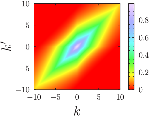
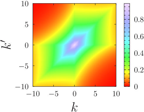
Several points have to be emphasised.
First, we notice that the result in (49) permits us to reproduce (32) in the particular case . Indeed, noticing that , we have
| (50) | |||||
which is precisely our result in (33), obtained by taking into account only the leading asymptotic behaviour of the Jacobi theta-function. This means, in turn, that the arguments used for the derivation of the result in (33) are correct.
Second, we notice that taking the limit and performing the summation operations can not be interchanged. Indeed, for any fixed and we have , which signifies, in turn, that for small the sums in (46) are dominated by the terms with large and . Further, since are linked
to the correlation function of the local occupation times at two different points, they depend simultaneously on both the distances and from this sites to the origin (the starting point of the trajectory ) and also on their relative distance . In these dependences, which are simple exponential functions for , the characteristic decay of with depends on both and and here we can safely set . On contrary, we have to keep the dependence of the characteristic decay length on in the terms dependent only on and (the sum of two exponential functions in the first factor in the right hand-side of (49).
5.2 Arbitrary .
We turn next to the general case of an arbitrary focussing on the diagonal terms. For , the couplings in (5) read
| (51) | |||||
It is convenient next to change the integration variables and and rewrite in (51) as
| (52) | |||||
where is defined in (13). Inspecting the integral over , we note that the cosine term oscillates heavily when is kept fixed and , which means that in this limit the integral over is concentrated in the vicinity of , i.e., for . Expanding then in the vicinity of ,
| (53) |
as well as other -dependent functions in the kernel and taking into account only the leading in this limit terms, we find that the integral in (52) can be approximately rewritten as
| (54) |
Performing then the integral over , we find
| (55) |
which form often arises in the analysis of various physical problems via the optimal fluctuation method (see, e.g., Ref. [52, 53]). On the other hand, the integral in (55) defines the so-called special Krätzel function (see, e.g., Ref. [54])
| (56) |
and therefore, the diagonal couplings can be formally represented as
| (57) |
Before we proceed to the analysis of the asymptotic behaviour of in (57), it seems expedient to consider first a particular case of Brownian motion (). Here, we have
| (58) |
such that
| (59) |
which expression agrees perfectly well with our previous result in (49) with set equal to . Further on, summing the expression in the second line in (55) over all , and taking an appropriate limit in the resulting Jacobi theta-function, we recover exactly our result in (32) for the disorder-averaged Wigner-Ville spectrum.
The -dependence of the diagonal couplings given in (57) is plotted in Fig. 4. The case of the Brownian motion, corresponding to (49) with , is depicted with a dotted line. We observe that upon increasing the Hurst index, the diagonal coupling increases monotonically for any , while for any fixed the large- behavior indicates the stretched-exponential decay predicted by the asymptotic result (• ‣ 5.2).

Lastly, we consider the asymptotic behaviour of in (57) in the limits and . For the sake of notational convenience, we rescale by defining .
- •
- •
Large- asymptotic behaviour. Recalling the properties of the Krätzel function summarised in Ref. [54], we find
(62) Therefore, the couplings in (57) exhibit a stretched-exponential dependence on both and
(63) In the particular case , the decay with in the latter expression becomes purely exponential. For super-diffusive fBm process , the decay of with is slower than exponential, i.e., with . On contrary, for sub-diffusive processes , vanishes faster than an exponential, with . In particular, for (the case of a tagged bead in an infinite Rouse polymer), one finds .
6 Conclusions
To recap, we have studied here a model of anomalous diffusion of a tracer particle in presence of stratified layers of quenched random flows. The particle undergoes a fractional Brownian (fBm) motion with the Hurst index in the direction perpendicular to the flows (along the -axis) and is passively advected in random directions (with no global bias) by the flows along the -axis. Averaging the squared displacement along the flows over the flow realisations, as well as over the fBm-trajectories, we obtained the mean-squared displacement along the flow direction and showed that for large times it grows in proportion to , which law defines a family of super-diffusive processes. In order to quantify the sample-to-sample fluctuations of the displacement along the random flow, we computed the coefficient of variation of the probability distribution function of the displacement. We showed that such fluctuations are typically not very important for but may become important for sufficiently small values of .
Next, we introduced the Wigner-Ville power spectral density (see (2) and (3)) of the random process and derived an exact result showing that the disorder-averaged Wigner-Ville spectrum scales with the frequency as , which defines a family of rather unusual super-diffusive spectra. To estimate the sample-to-sample fluctuations of the spectrum, we examined the limit of zero frequency of the Wigner-Ville spectrum averaged over a finite time interval of duration . We found that the ratio of the standard deviation of the spectrum and of the mean value diverges with , which implies that the distribution of the spectrum with respect to different realisations of disorder progressively broadens with the observation time.
Lastly, representing the Wigner-Ville spectrum of the process for a given realisation of flows as an Ising-like model of ”spins” , which define the local direction of the flows along the -axis, we have analytically determined the coupling terms in this model, in the Laplace domain. In particular, we showed that the latter exhibit a non-trivial dependence on the distance from the origin and the Laplace parameter.
In general, our analysis reveals that sample-to-sample fluctuations are important, both for the dynamical characteristics and the spectral behaviour. This issue is beyond the scope of the current work and will be examined elsewhere.
References
References
- [1] B. Mandelbrot, Some noises with spectrum, a bridge between current and white noise, IEEE Trans. Inf. Theory 13, 289 (1967).
- [2] R. M. Loynes, J. Roy. Stat. Soc. B 30, 1 (1968).
- [3] W. Martin and P. Flandrin, IEEE Trans. Acoust., Speech, Sig. Proc. ASSP-33, 1461 (1985).
- [4] P. Flandrin, IEEE Trans. Inf. Theory 35, 197 (1989).
- [5] N. Leibovich, A. Dechant, E. Lutz and E. Barkai, Phys. Rev. E 94, 052130 (2016).
- [6] D. Krapf et. al, New J. Phys. 20 023029 (2018).
- [7] D. Krapf et. al, Phys. Rev. X 9 011019 (2019).
- [8] , V. Sposini, R. Metzler and G. Oshanin, New J. Phys. 21, 073043 (2019)
- [9] P. Dutta and P. M. Horn, Low-frequency fluctuations in solids: noise, Rev. Mod. Phys. 53, 497 (1981).
- [10] E. Marinari, G. Parisi, D. Ruelle, and P. Windey, Phys. Rev. Lett. 50, 1223 (1983).
- [11] E. Marinari, G. Parisi, D. Ruelle, and P. Windey, Commun. Math. Phys. 89, 1 (1983).
- [12] V. Sposini, D. S. Grebenkov, R. Metzler, G. Oshanin and F. Seno, Universal spectral behaviour for a variety of diffusing diffusivity models, in preparation
- [13] O. Bénichou, P.L. Krapivsky, C. Mejia-Monasterio and G. Oshanin, Phys. Rev. Lett. 117, 080601 (2016).
- [14] D. S. Dean, A. Iorio, E. Marinari and G. Oshanin, Phys. Rev E 94, 032131 (2016).
- [15] A. Sornette and D. Sornette, Europhys. Lett. 9, 197 (1989).
- [16] B. B. Mandelbrot and J. R. Wallis, Water Resour. Res. 5, 321 (1969).
- [17] J. M. Halley, Ecology, evolution and noise, Trends Ecology Evol. 11, 33 (1996).
- [18] D. L. Gilden, T. Thornton and M. W. Mallon, Science 267, 1837 (1995).
- [19] I. Csabai, J. Phys. A: Math. Theor 27, L417 (1994).
- [20] S. N. Majumdar and G. Oshanin, J. Phys. A: Math. Theor. 51, 435001 (2018).
- [21] W. H. Press, Comments Astrophys. Space Phys. 7, 103 (1978).
- [22] S. M. Bezrukov and M. Winterhalter, Phys. Rev. Lett. 85, 202 (2000).
- [23] Z. Siwy and A. Fulinski, Phys. Rev. Lett. 89, 1 (2002).
- [24] D. Krapf, Phys. Chem. Chem. Phys. 15, 459 (2013).
- [25] A. R. Bizzarri and S. Cannistrato, Phys. Rev. Lett. 110, 048104 (2013).
- [26] S. Sadegh, E. Barkai and D. Krapf, New J. Phys. 16, 113054 (2014).
- [27] E. W. Montroll and M. F. Shlesinger, Proc. Natl. Acad. Sci. USA 79, 3380 (1982).
- [28] M. Niemann, H. Kantz and E. Barkai, Phys. Rev. Lett. 110, 140603 (2013).
- [29] N. Leibovitch and E. Barkai, Phys. Rev. Lett. 115, 080602 (2015).
- [30] Yu. A. Dreizin and A. M. Dykhne, Sov. Phys. JETP 36, 127 (1973).
- [31] G. Matheron and G. de Marsily, Water Resources Res. 16, 901 (1980).
- [32] S. Redner, Physica A 168, 551 (1990).
- [33] P. Le Doussal and J. Machta, Phys. Rev. B 40, 9427 (1989).
- [34] J. P. Bouchaud, A. Georges, J. Koplik, A. Provata, and S. Redner, Phys. Rev. Lett. 64, 2503 (1990).
- [35] G. Zumofen, J. Klafter and A. Blumen, Phys. Rev. A 42, 4601 (1990).
- [36] P. Le Doussal, J. Stat. Phys. 69, 917 (1992).
- [37] J. Klafter, M. Shlesinger, G. Zumofen and A. Blumen, Phil. Mag. B 65, 755 (1992).
- [38] A. Crisanti and A. Vulpiani, J. Stat. Phys. 70, 197 (1993).
- [39] S. N. Majumdar, Phys. Rev. E 68, 050101 (2003).
- [40] S. Roy and D. Das, Phys. Rev. E 70, 026106 (2006).
- [41] G. Oshanin and A. Blumen, Phys. Rev. E 49, 4185 (1994); Macromol. Theory Simul. 4, 87 (1995).
- [42] K. J. Wiese and P. Le Doussal, Nucl. Phys. B 552, 529 (1999).
- [43] S. Jespersen, G. Oshanin and A. Blumen, Phys. Rev. E 63, 011801 (2001).
- [44] S. N. Majumdar and D. Das, Phys. Rev. E 71, 036129 (2005).
- [45] C. Maes and S. R. Thomas, Phys. Rev. E 87, 022145 (2013).
- [46] D. Katyal and R. Kant, Phys. Rev. E 91, 042602 (2015).
- [47] B. Mandelbrot and J. W. van Ness, SIAM Review 10, 422 (1968).
- [48] S. N. Majumdar, Curr. Sci. 77, 370 (1999).
- [49] S. N. Majumdar and A. Comtet, Phys. Rev. Lett. 89, 060601 (2002).
- [50] C. Mejía-Monasterio, G. Oshanin and G. Schehr, J. Stat. Mech. (2011) P06022.
- [51] T. Mattos, C. Mejía-Monasterio, R. Metzler and G. Oshanin, Phys. Rev. E 86, 031143 (2012).
- [52] C. Monthus, G. Oshanin, A. Comtet and S. F. Burlatsky, Phys. Rev. E 54, 231 (1996).
- [53] S. B. Yuste, G. Oshanin, K. Lindenberg, O. Bénichou and J. Klafter, Phys. Rev. E 78, 021105 (2008).
- [54] A. A. Kilbas, L. Rodríguez-Germá, M. Saigo, K. Saxena and J. J. Trujillo, Comput. Math. Appl. 59, 1790 (2010).
- [55] A. Hatzinikitas and J. K. Pachos, Ann. Phys. 323, 3000 (2008).