Optimal Rates for Learning Hidden Tree Structures
Abstract
We provide high probability finite sample complexity guarantees for hidden non-parametric structure learning of tree-shaped graphical models, whose hidden and observable nodes are discrete random variables with either finite or countable alphabets. We study a fundamental quantity called the (noisy) information threshold, which arises naturally from the error analysis of the Chow-Liu algorithm and, as we discuss, provides explicit necessary and sufficient conditions on sample complexity, by effectively summarizing the difficulty of the tree-structure learning problem. Specifically, we show that the finite sample complexity of the Chow-Liu algorithm for ensuring exact structure recovery from noisy data is inversely proportional to the information threshold squared (provided it is positive), and scales almost logarithmically relative to the number of nodes over a given probability of failure. Conversely, we show that, if the number of samples is less than an absolute constant times the inverse of information threshold squared, then no algorithm can recover the hidden tree structure with probability greater than one half. As a consequence, our upper and lower bounds match with respect to the information threshold, indicating that it is a fundamental quantity for the problem of learning hidden tree-structured models. Further, the Chow-Liu algorithm with noisy data as input achieves the optimal rate with respect to the information threshold. Lastly, as a byproduct of our analysis, we resolve the problem of tree structure learning in the presence of non-identically distributed observation noise, providing conditions for convergence of the Chow-Liu algorithm under this setting, as well.
keywords
Tree-structured graphical models, Chow-Liu algorithm, Information Threshold, Hidden Markov models, Noisy data1 Introduction
Graphical models are a widely-used and powerful tool for analyzing high-dimensional structured data (Lauritzen 1996; Koller and Friedman 2009). In those models, variables are represented as nodes of a graph, the edges of which indicate conditional dependencies among the corresponding nodes. In this paper, we consider the problem of learning acyclic undirected graphs or tree-structured Markov Random Fields (MRFs). In particular, we provide optimal rates for the problem of learning tree structures under minimal assumptions, when noisy data are available. First, we analyze the sample complexity of the well-known Chow-Liu (CL) Algorithm (Chow and Liu 1968), which, given a data set of samples, returns an estimate of the original tree. In the absence of noise the importance of the CL algorithm stems from its efficiency, its low computational complexity, and also its optimality in terms of sample complexity (matching information-theoretic limits) for a variety of statistical settings, e.g., such as those involving Gaussian data (Tan et al. 2010), binary data (Bresler and Karzand 2020), as well as for non-parametric models with discrete alphabets (Tan et al. 2011a; Tan et al. 2011b). Second, the CL algorithm with noisy data as input maintains its computational efficiency, and as we show, achieves optimal sample complexity rates for certain cases of hidden tree-structured models
In many applications, the underlying physical or artificial phenomenon may be well-modeled by a (tree-structured) MRF, but the data acquisition device or sensor may itself introduce noise. We wish to understand how sensitive the performance of an algorithm is to noisy inputs. The problem of learning hidden structures receives significant attention the last few years. Prior or concurrent works include partial Tandon et al. 2020; Katiyar et al. 2020; Tandon et al. 2021; Casanellas et al. 2021; Katiyar et al. 2021, as well as exact structure recovery (Goel et al. 2019; Nikolakakis et al. 2019; Nikolakakis et al. 2021). Specifically, Goel et al. 2019; Nikolakakis et al. 2019 study the impact of corrupted observations on the exact recostruction for both binary and Gaussian models. Goel et al. 2019 extend the Interaction Screening Objective (Vuffray et al. 2016) for the case of Ising models, while our prior work (Nikolakakis et al. 2019) analyzes the performance of the CL algorithm for both noisy Ising and Gaussian models. Based on this prior work, it is tempting to think that one can successfully perform structure recovery by running the standard CL algorithm directly on noisy data, for general hidden tree-models and minimal assumptions.
Our contribution centers on a rigorous characterization of a fundamental model-dependent statistic, which we call the information threshold (denoted by and for the noiseless and noisy settings, respectively). For the problem of learning tree-structures from noiseless data, the information threshold has already appeared in fundamental prior work in the area (e.g., see prior work by Tan et al. 2011 and Tan 2011). Precisely, Theorem 6 by Tan et al. 2011 states that if the information threshold is strictly positive, then the probability of incorrect structure recovery by the CL algorithm decays exponentially with respect to the number of samples. Specifically, Tan et al. 2011a; Tan et al. 2011 show that the approximation of the error exponent is consistent with the true error exponent when . However, no conclusions can be derived based on results from prior works regarding the rate of the sample complexity with respect to when it is bounded away from zero, or when the data are noisy.
In this paper, we provide finite sample complexity bounds for exact hidden tree-structure learning. Although it is true that the number of samples required for successful recovery scales logarithmically with respect to the number of nodes (in the asymptotic sense), the sample complexity can vary significantly for different tree-structured distributions or noise models (for fixed ), and fixed probability of failure . The discussion above naturally raises the following basic question: Is there any essential statistic (e.g., the information threshold) that determines the sample complexity of the hidden tree-structure learning problem? We show that, indeed, the noisy information threshold constitutes such a representative statistic; in fact, it provides explicit necessary and sufficient conditions on sample complexity, by effectively and completely summarizing the difficulty of the hidden tree-structure learning problem. First, for fixed positive values of probability of success and (noisy) information threshold (namely ), we derive finite complexity bounds for exact structure recovery, by exploiting the Chow-Liu algorithm with noisy observations as its inputs. Second, we show that our sample complexity bounds achieve the optimal rate with respect to .
Our contributions are summarized as follows.
- •
We provide the first finite sample complexity results on non-parametric hidden tree-structure learning, where the distributions of the hidden and observable layers are unknown and the mappings between the hidden and observed variables are general. In fact, as with the noiseless case, we show that, as long as , the sample complexity of the CL algorithm with respect to scales as , for any . With respect to the associated noisy information threshold, the same sample complexity is of the order of , for any (Theorem 10).
- •
For an absolute constant , we show that if the number of samples is less than , then no algorithm can recover the hidden tree structure with probability greater than one half (Theorem 14). The rate of of upper and lower bounds with respect to are essentially identical, and CL algorithm in the noisy setting achieves the optimal rate with respect to .
- •
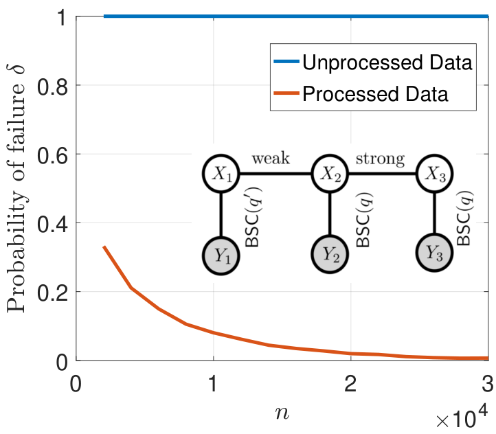
Additionally, we show that, if , then structure recovery from raw data is not possible. As an example of the case consider the model in Figure 1, for which structure recovery from unprocessed data fails. In some cases where , by introducing suitable processing and enforcing appropriate conditions on the hidden model (Definition 15), we show that the CL algorithm can be made convergent (with the aforementioned sample complexity). Such conditions can be satisfied for a variety of interesting observation models. Essentially, our results confirm that the CL algorithm is an effective universal estimator for tree-structure learning, on the basis of noisy data. We lastly explicitly illustrate how our results capture certain interesting scenarios involving generalized -ary erasure and symmetric channels (i.e., observation noise models). Our framework extends and unifies recent results proved earlier for the binary case (Bresler and Karzand 2020; Nikolakakis et al. 2019), by considering non-identically distributed noise as well. Note that structure learning in the presence of non-identically distributed noise remains open for general graph structures; see prior work by Goel et al. 2019.
1.1 Related Work
Structure learning from node observations is a fundamental and well-studied problem in the context of graphical models. For general graph structures, the complexity of the problem has been studied by Karger and Srebro 2001. Under the assumption of bounded degree the problem becomes tractable, leading to a large body of work in the last decade (Vuffray et al. 2016; Lee et al. 2006; Bresler et al. 2008; Ravikumar et al. 2010; Bresler et al. 2014; Bresler 2015; Vuffray et al. 2019). These approaches employ greedy algorithms, regularization methods, or other optimization techniques. The sample complexity of each approach is evaluated based on information theoretic bounds (Santhanam and Wainwright 2012; Tandon et al. 2014; Hamilton et al. 2017).
For acyclic graphs, the CL algorithm is computationally efficient and it has been shown to be optimal in terms of sample complexity with respect to the number of variables. The error analysis and convergence rates for trees and forests were studied by Tan et al. 2010; Tan et al. 2011a; Tan et al. 2011b, Liu et al. 2011 and Bresler and Karzand 2020. In particular, for finite alphabets the number of samples needed by the CL algorithm is logarithmic with respect to the ratio for tree structures and polylogarithmic in the case of forests: , for all (Tan et al. 2011b, Theorem 5)). Comparatively, our results extend to countable alphabets and noisy observations (hidden models). Our sample complexity bounds are consistent with prior work: the order is poly-logarithmic but remains arbitrarily close to logarithmic (, for all ). In the special case of Ising models, hidden structures were considered by Goel et al. 2019 and our previous work (Nikolakakis et al. 2019; Nikolakakis et al. 2021). Goel et al. (Goel et al. 2019) consider bounded degree graphs and require the noise model (or an approximation of it) to be known with the noise i.i.d. on each variable (see their Section 6). Our results apply more generally to settings with non-identically distributed noise (Section 5.1.2), but are restricted to the tree structure model assumption. Prior work by (Nikolakakis et al. 2019; Nikolakakis et al. 2021) solves the problem of hidden tree structure learning for (binary) Ising models with (modulo-2) additive noise, while in this paper we generalize prior sample complexity bounds (Nikolakakis et al. 2019; Nikolakakis et al. 2021) to finite and countable alphabets, encompassing non-parametric tree structures and general noise models. Finally, Tandon et al. 2020; Katiyar et al. 2020; Tandon et al. 2021; Casanellas et al. 2021; Katiyar et al. 2021 consider the problem of learning hidden tree-structured models within an equivalence class. In contrast with these papers, we study the exact structure recovery instead of that of the partial structure learning.
1.2 Applications
Noise-corrupted structured data appear in various applications for major branches of science as physics, computer science, biology and finance. The assumption of discrete and (arbitrarily) large alphabets is suitable for many of these scenarios. Our work is also motivated by a number of emerging applications in machine learning: differential privacy, distributed learning, and adversarial corruption. For example in local differential privacy (Warner 1965; Evfimievski et al. 2003; Kasiviswanathan et al. 2008; Kasiviswanathan et al. 2011; Duchi et al. 2013; Smith et al. 2017), one approach perturbs each data sample at the time it is collected: our results therefore characterize the increase in sample complexity for successful structure recovery under a given privacy guarantee. In distributed learning problems, communication constraints require data to be quantized, resulting in quantization noise on the samples (c.f. (Tavassolipour et al. 2019)). Finally, we might have an adversarial attack on the training data: an adversary could corrupt the data-set and make structure learning infeasible. As our example shows, non-i.i.d. corruption can make the information threshold negative, and the CL algorithm will fail without appropriate processing of the mutual information estimates. We continue by introducing the notation that we use in our paper.
1.3 Notation
We denote vectors or tuples by using boldface and we reserve calligraphic face for sets. For an integer , let , and let denote the corresponding Cartesian product. For an odd natural number , we denote the set of even natural numbes up to as . The indicator function of a set is denoted by . In our graphica models, the cardinality of the set of nodes is assumed to be equal to , . The node variables of the tree are denoted by . If has a finite alphabet we write , and for countable size alphabets. The probability mass function of is denoted by and the joint distribution of the pair by , for any . is a tree (acyclic graph) with set of nodes and edges and respectively. We denote the unique set of edges in the path of two nodes of as . The neighborhood of a node is denoted by . The distribution is the estimator of a distribution . The symbol denotes the dataset of i.i.d samples of . The estimated mutual information of a pair is and the resulting tree structure of the CL algorithm is denoted by . The noisy observable is denoted by and we use the symbol to distinguish between noiseless quantities and the corresponding noisy quantities, for instance is the estimated tree from .
2 Model and Problem Statement
First, we provide a complete description of our model including definitions, properties, and assumptions on the underlying distributions.
2.1 Tree-Structured and Hidden Tree-Structured Models
We consider graphical models over nodes with variables and finite or countable alphabet . We assume that the distribution of is given by a tree-structured Markov Random Field, (MRF). Any distribution which is Markov with respect to a tree factorizes as (Lauritzen 1996)
| (1) |
we call such distributions tree-structured.
The noisy node variables are generated by a randomized mapping (noisy channel) . We restrict attention here to mappings that act on each component (not necessarily independently): and each so for all . Let be the transition kernel associated with the randomized mapping , then the distribution of the output is given by for . Note that while the distribution of is tree-structured, the distribution of does not factorize according to any tree. In general the Markov random field of is a complete graph, which makes learning the hidden structure non-trivial (Nikolakakis et al. 2019; Nikolakakis et al. 2021; Yeung et al. 2018).
Given i.i.d observations , our goal is to learn the underlying structure . To do this, we use a plug-in estimate of the mutual information between pairs of variables. In similar fashion, when noise-corrupted observations are available, we aim to learn the hidden tree structure of , by estimating the mutual information between pairs of observable variables. Unfortunately, the plug-in mutual information estimate may converge slowly to in certain cases with countable alphabets (Antos and Kontoyiannis 2001, Corollary 5), (Silva 2018). To avoid such ill-conditioned cases, we make the following assumption.
Assumption 1.
For some there exist such that , for , and , for and for all . That is, the tuple satisfies the assumption for all marginal and pairwise joint distributions.
Assumption 1 holds trivially for all finite and (fixed) alphabets, where the constants and depend on the minimum probability and the size of alphabet. The next assumption guarantees there is a unique tree structure with exactly nodes.
Assumption 2.
is connected; for all and the distribution of is not degenerate.
Assumption 2 guarantees convergence for the CL algorithm in the absence of noise; . For a fixed tree , we use the notation to denote the set of structured distributions that factorizes according to a fixed . The set of all trees on nodes is denoted by , and we call the set of all tree-structured distributions that factorize according to (1) for some .
2.2 Chow-Liu Algorithm
We consider the classical version of the algorithm (Chow and Liu 1968), due to the non-parametric nature of our model. Given i.i.d samples of the node variables, we first find the estimates of the pairwise joint distributions and then we evaluate the plug-in mutual information estimates. Finally, a Maximum Spanning Tree (MST) algorithm (for instance Kruskal’s or Prim’s algorithm) returns the estimated tree. For the rest of the paper, we refer to Algorithm 1 by explicitly mentioning the input data set; if , then the input consist of noiseless data and we consider (see Algorithm 1), furthermore the estimated structure is denoted by . Equivalently, if , then the input consists of noisy data, , and the estimated structure is named as . We compute and by running the MST algorithm on the edge weights and respectively. Note that the estimates and depend on the value , but for brevity, we write and instead of and respectively. In the next section we show that Chow-Liu algorithm is equivalent to a maximum likelihood estimator: Algorithm 1 returns the MLE-tree of the projected distribution of the observables onto the space of tree-structured distributions.
2.3 Projected Maximum Likelihood Estimate
We now show the connection between the maximum likelihood estimate tree and the output of Chow-Liu algorithm with input noisy data. As a first step, we state the following Lemma, that generalizes the result on Ising model distribution by Bresler and Karzand 2020 to general distributions.11 1 We are unaware of a prior proof of the following result and so we provide it for completeness.
Lemma 1.
Let be a distribution that factorizes according a graph , and a tree structured distribution with , such that is absolutely continuous with respect to . Let be the mutual information with respect to and consider the projection of onto the space of tree-structured distributions
| (2) |
Then
| (3) |
Proof.
It is true that
| (4) | ||||
| (5) |
At this point the following notation is necessary (see (Koski 2010)): Let be an arbitrary permutation of . Then, the set of edges for any tree can be written as
| (6) |
(6) defines a tree with root the node (since ). Then we write (5) as
| (7) |
Notice that
| (8) |
and
| (9) |
because of the monotonicity property of the KL divergence. Thus to minimize (7) we need the equality to hold in (8) and (9). Under the choice of as the projection onto the space of tree structured distributions as , we get the matching on the distribution of the root and the matching on the pairwise marginal distributions for all , or equivalently for all (see (6)). The latter makes the KL divergences equal to zero in (8) and (9), and (7) directly gives (3). ∎
The true distribution of the observable layer and the estimated distribution from i.i.d noisy samples do not factorize according to any tree. Although the noisy data do not come from a tree-structured distribution (in contrast with prior work (Tan et al. 2011a)), the approach by Tan et al. 2011a can be extended as follows. Given i.i.d noisy samples from a hidden tree-structured model, Chow-Liu algorithm (Algorithm 1) with input returns the maximum likelihood estimate tree of the projected distribution
| (10) |
Corollary 2.
The maximum likelihood estimate tree of is equivalent with the output of Chow-Liu algorithm, that is,
| (11) |
Proof.
Although Corollary 2 indicates optimality of the algorithm in some cases, it is well-known that under the presence of noise an MLE approach may be non-robust. To mitigate the effect of noise extra steps should be considered such as pre-processing, statistical learning of the noise by using pilot samples, or detecting and rejecting bad samples; see also Zoubir et al. 2012. When the CL algorithm is not consistent, we later discuss how appropriate processing procedures can provide a consistent variation of the algorithm for specific hidden models (Section 5).
2.4 Analysis of the Error Event
We continue by analyzing the event of incorrect reconstruction (or ), which yields a sufficient condition for exact structure recovery.
Proposition 3.
The estimated tree if and only if there exist two edges and such that , and . Then also .
Intuitively, exact recovery fails when there is at least one edge in the original tree which does not appears in the estimated tree . We refer the reader to the proof of Proposition 3 by Bresler and Karzand 2020. For sake of space, we define the set .
Definition 4 (Feasibility set ).
Let be an edge and be a pair of nodes such that and . The set of all such tuples , is defined as
| (15) |
For the rest of the paper the pair of nodes , denotes the edge . The error characterization of CL algorithm is expressed as follows: if then there exists such that22 2 The event has non zero probability for certain cases, in this situation the MST arbitrarily chooses one of the edges . The choice of yields the error event .
By negating the above statement, we get that if for all then . The latter yields a sufficient condition for accurate structure estimation.
Sufficient condition for exact structure recovery: For exact structure recovery we need for all , or equivalently
| (16) |
Inequality (16) allows us to derive a sufficient condition based on error estimates of the mutual information as follows.
Proposition 5.
If
| (17) |
for all then .
2.5 Information Threshold and Properties
We now define our quantity of interest for tree structured distributions, which we call the information threshold. As well will see shortly, our sample complexity bounds for exact structure recovery via the CL algorithm depend on the distribution only through the information threshold, . We first define and then show how it affects the difficulty of the structure estimation problem.
Definition 6 (Information Threshold (IT)).
Let be an edge and be a pair of nodes such that . The information threshold associated with the model (see Section 2.1) is defined as
| (18) |
The minimization in (17) and (18) is with respect to the feasible set of the hidden tree structure of . Note that the distribution of does not factorize according to any tree (Yeung et al. 2018), thus it is possible to have .
When the data are noiseless, the gap between mutual informations that defines the information threshold will change. If the errors of the mutual information estimates of the noiseless variables satisfy the condition
| (19) |
for all then , and (19) is derived similarly to (17). The definition of the noiseless information threshold naturally results from the previous condition.
Definition 7 (Noiseless IT).
The noiseless information threshold is defined as
| (20) |
Similarly to the noisy case, if
| (21) |
then . The data processing inequality (Cover and Thomas 2012) shows that . Also, Assumption 2 guarantees that .
Proposition 8 (Positivity).
If Assumption 2 holds then .
Since the values for are constant relative to (Tan et al. 2011b), does not depend on . The latter holds because of the locality property of .
Proposition 9 (Locality).
3 Recovering the Structure from Noisy Data
We start by developing a finite sample complexity bound for exact structure learning with high probability, when noisy data are available. The structure learning condition in (21), combined with results on concentration of mutual information estimators (Antos and Kontoyiannis 2001), yields the following result.
Theorem 10 (General Alphabets).
Remarks: First, the constant depends on the values of constants which are defined in Assumption 1. Specifically, . The derivation of has been given by Antos and Kontoyiannis (Antos and Kontoyiannis 2001, Theorem 7). Additionally, note that for any fixed . Therefore, the required number of samples with respect to and and for fixed scale as , for any choice of , whereas, for fixed and , the complexity is of the order of is , for any . The proof of Theorem 10 now follows.
Proof of Theorem 10.
To calculate the probability of the exact structure recovery we use a concentration inequality quantifying the rate of convergence of entropy estimators from Antos and Kontoyiannis (Antos and Kontoyiannis 2001). In particular, they show ((Antos and Kontoyiannis 2001, Corollary 1)) how the plug-in entropy estimator (say) is distributed around its mean : For every and ,
| (24) |
The plug-in entropy estimator is biased and, actually, . Under their Assumption 1, in Theorem 7 (Antos and Kontoyiannis 2001) they characterize the bias as follows. For (which is the case of interest in this proof),
| (25) |
and for ,
| (26) |
Then, for , it is true that
| (27) |
and the last inequality comes from (24) and (25). Notice that for non-trivial bounds we need the condition . Further, is free parameter and we choose , driven by property (19). This requires than has to be sufficiently large, such that the following inequality holds
| (28) |
Our goal is to find an upper on the probability of the event . By combining the above and applying the property we have
| (29) |
where the last inequality is a consequence of (27). To guarantee that the condition in (19) holds, we apply the union bound on the events , for all . Since there are pairs we define
| (30) |
To conclude, for some fixed if
| (31) |
then the probability of exact recovery is at least . The latter combined with the inequalities , gives
| (32) |
thus it sufficient to have
| (33) | ||||
| (34) |
The last statement gives the statement of the theorem. ∎
Theorem 10 characterizes the sample complexity for models with either countable or finite alphabets. By restricting our setting to finite alphabets Assumption 1 is not required and we have the following result. The proof is virtually identical to that of Theorem 10, and is omitted.
Theorem 11 (Finite Alphabets).
Lastly, the corresponding variation of Theorem 10 when Assumption 1 holds for (in the general case of countable alphabets) follows.
Theorem 12 (Countable Alphabets, ).
Assume that . Assume that noisy data are generated by a randomized set of mappings , and satisfies the Assumption 1 for some . Fix . There exists a constant independent of such that, if and the number of samples of satisfies the inequalities
| (36) |
then Algorithm 1 with input the noisy data returns with probability at least .
As a byproduct of our analysis we also derive the sample complexity bound for the noiseless case as well. Now the bound involves the (noiseless) information threshold .
Theorem 13.
Assume that and satisfies the Assumption 1 for some . Fix a number . There exists a constant , independent of such that, if the number of samples of satisfies the inequality
| (37) |
then Algorithm 1 with input returns with probability at least . The relationship between and is given similarly to that of Theorem 10.
This result allows us to compare the sample complexity of the noiseless and noisy setting. Let and denote the sufficient number of samples of and respectively and consider fixed, then the ratio is for all . The latter shows how changes relative to under the same probability of success for both settings (noiseless and noisy). The proof of Theorem 13 is similar to the proof of Theorem 10.
Proof of Theorem 13.
The difference is introduced by the event in (21). That is, the error on the mutual information estimates should be less than the noiseless information threshold . Note that for the entropy estimates of , equations (24) up to (27) hold with possibly different constants than those of the observable layer (see Assumption 1). Here we consider the case where (the case is similar, see also the proof of Theorem 10), and the corresponding bound on the estimation error has to be at most . Thus, (28) becomes
| (38) |
and (29) now is written as
| (39) |
Finally, by applying union bound over the pairs we derive the statement of Theorem 10, by following the equivalent steps of (30) and (31). The latter completes the proof. ∎
4 Converse: Information Threshold as a Fundamental Quantity
In this section we provide the statement of the converse of our main result Theorem 10. We define the class of hidden tree-structured models with bounded (from below) information threshold of the hidden layer by an absolute positive constant and bounded absolute information threshold for the observable layer by a fixed as33 3 The information threshold of the observable layer can be either positive or negative for each model in the class .
| (40) |
The next result provides a lower bound for the necessary number of samples for tree-structure learning from noisy observations.
Theorem 14.
There exist absolute constants such that for any and for any estimator , if , then the worst-case probability of incorrect structure recovery over all hidden tree-structured models in is at least . In other words, it is true that if , then
| (41) |
Additionally, the supremum is attained.
Proof of Theorem 14.
We define the set of hidden tree-structured models , and (see Figure 2) as follows: The hidden layer of is , and , the hidden layer of is and , the hidden layer of is and . Further for all models, for and for any and . Note that the information threshold of the hidden layer is strictly positive for any , since
| (42) |
and by construction , . The observable data are generated by binary symmetric channels with cross-over probabilities , and and . The binary noise variables are multiplicative, independent from each other and independent from the hidden variables and generate the corresponding observable as (see Figure 2). Specifically, for the model we have and , for the model and , and for the model and .44 4 The construction of the hidden models is similar to Bhattacharyya et al. 2020. The crucial difference is that our construction involves hidden layers with , while in their Lemma 7.1 the information threshold of the hidden is zero and the construction is inappropriate for the structure learning problem.
The distribution of any pair is
| (43) |
We find the second order moments of the model as follows:
| (44) | ||||
| (45) | ||||
| (46) | ||||
| (47) | ||||
| (48) |
We combine the above and we choose to evaluate the information threshold
| (49) |
Similarly for the model ,
| (50) | ||||
| (51) | ||||
| (52) | ||||
| (53) | ||||
| (54) |
The information threshold is
| (55) |
As a consequence, (49) and (55) give and . In contrast, (42) gives . Further, the joint distributions of the models are given by
| (56) |
| (57) |
and for both (56), (56) . We use (56) and (57) to evaluate the probabilities
By the definition of the KL divergence
| (58) |
Similarly for the model we have
| (59) |
| (60) |
and we find
| (61) |
Next, we use Fano’s inequality (see Tsybakov 2009). Fix and let , denote the probability laws of under models and respectively, and consider i.i.d. observations . If
| (62) |
with then
| (63) |
where the infimum is relative to all estimators (statistical tests) . Specifically, for and
| (64) |
if
| (65) |
then
| (66) |
Finally, , from (58), (61) and , , from (49), (55), (59). Thus there exists and such that for any it is true that . Then the statement of the theorem follows.∎
5 Inconsistency of CL Algorithm and the Effect of Pre-Processing
The information threshold in (20) appears in the condition for exact structure recovery using the CL algorithm (19): Algorithm 1 is consistent as long as . To be more precise, for every there exists such that if then (19) holds with high probability. In fact, in Theorem 10 the condition is necessary. Under the assumption of (see Assumption 2), it is not guaranteed that . If then the CL is not consistent in the sense that
| (67) |
On the other hand if , then ties are broken arbitrarily and the probability of missing an edge does not decrease as increases. In what follows, we provide sufficient conditions which ensure that . In particular, whenever , we show that for certain hidden models, an appropriate processing can be introduced as an extra step to overcome the inconsistency of the CL algorithm. As a result, the output of CL algorithm under the appropriate processing will converge to the original tree of the hidden layer.
First observe that if for all pairs of nodes the inequalities and simultaneously hold, then . The last statement yields the required processing for the cases for which the algorithm is not consistent. Specifically, we would like to find weights , that we consider as new input of the maximum spanning tree in Algorithm 1.
Definition 15.
A processing procedure with input noisy data, is called appropriate if it returns a set of edge weights , and there exists such that for every and every tuple
| (68) |
Such processing procedures are inherently model-based, and the required processing is tied to the underlying hidden model. In the next section, we show that in different models of interest, the noise can affect the original edge weights in dissimilar ways; in fact, whether there exist universal rules for processing procedures for large classes of hidden models is currently unknown, and is an interesting problem for future work.
5.1 Relaxing the Condition for Two Non-Trivial Channels
To illustrate the case where , we present and discuss scenarios of interest that involve hidden tree-structured models for which Algorithm 1 succeeds with high probability, only if an appropriate processing is being applied. Specifically, we provide rules for identifying the feasibility of structure recovery. In contrast with the condition , these rules do not require knowledge of the structure or the unknown value beforehand. As a special case, the models in Sections 5.1.1 and 5.1.2 with identically distributed noise always satisfy the conditions, and no processing is required. On the other hand, for non-identically distributed noise, structure learning from raw data may be infeasible. We show how to distinguish such models and we provide the appropriate processing under the cases of interest.
5.1.1 Tree-Structured Binary Data with Non-Identically Distributed Noise
Consider the hidden tree structure with hidden nodes and observable nodes such that and , for all . The distribution of the noise is not identically distributed as
| (69) |
If for any tuple then the CL is not consistent (see (67)), and (84) gives
| (70) |
The inequality above involves the set , that is associated with the unknown tree structure. Thus we cannot check if (70) holds before running the CL algorithm. However, we show that we can relax the above condition as
| (71) |
and then . The proof of (71) is given in Appendix B.2. Condition (71) provides a testing rule for the feasibility of tree-structure estimation directly from raw noisy data. The advantage of (71) is that it does not involve any structure related information. On the other hand, it requires the knowledge of the noise parameters and the maximum correlation among the hidden nodes, or some accurate estimates of these parameters. Note that for identical noise , it is true that for all , thus (71) is always satisfied because , and structure learning is always feasible for this regime.
If condition (71) is not satisfied then structure recovery is still feasible by applying an appropriate pre-processing on the data . The pre-processing procedure requires the values (or estimates of them) to be known. By considering the pre-processing on the input data of Algorithm 1, the new weights are . The latter enforces an appropriate processing (see Definition 15) and guarantees that the algorithm is consistent,
| (72) |
Simulations on synthetic data verify our analysis (see Figure 3).
5.1.2 -ary Erasure Channel with Non-Identically Distributed Noise
Assume that the randomized mappings “erase” each variable independently with probability , so for all , we have with probability and (an erasure) with probability . Then for all (see Appendix B.1) and . The latter guarantees that if then . Given the values of and , Theorem 10 provides the sample complexity for exact structure recovery from noisy observations. For fixed values of and , the ratio of sufficient number of samples in the noiseless and noisy settings is , for any .
In contrast, consider the scenario where the erasure probability is not the same for every node (non-identically distributed noise). Each erases the node value with probability , so for all , and the condition shows that Algorithm 1 with input converges; , if for all tuples
| (73) |
Define . Inequality (73) provides the following simplified sufficient condition for convergence of CL Algorithm with input noisy data; if for all
| (74) |
However, (74) is not useful because the quantity involves knowledge related to the unknown tree structure. Thus is not possible to check if (74) holds before running the Chow-Liu algorithm. For that reason we would like to derive a relaxed version. To find a relaxed condition, we restrict the class of interest by introducing the following assumptions on the hidden layer :
- •
For a fixed known value , it is true that .
- •
For a fixed known value the inequality holds for all .
Then condition (74) can be relaxed as
| (75) |
Given the values and , or accurate estimates of them, (75) provides a rule for testing if structure estimation is possible directly from raw noisy data. Additionally, the above assumption on and for edge pairs is equivalent with an assumption on strong and weak edges of the tree, which is common in the literature (for instance see related work by Bresler and Karzand 2020.)
If direct structure estimation is not possible then we can consider an appropriate processing by considering as edge weights the values . Under the new input of the MST, the algorithm becomes consistent by satisfying the property of the appropriate processing in Definition 15. On the other hand, for identical distributed noise for each observable node (, for all ), the condition (75) always holds, thus structure recovery is always possible for identically distributed noise. Lastly, a comparison of the required processing for erasure channels and binary symmetric channels with non-identically distributed noise (Section 5.1.1), indicates that different processing procedures are required for different models.
6 Simulations
In this Section, we provide simulations to illustrate the dependence between the error rate and the corresponding value of the information threshold. For the simulations of this paper, the tree-structured of the hidden layer is generated randomly. Starting from the root, we choose the parent of each new node uniformly at random among the nodes that are currently in the tree, in a sequential fashion. To demonstrate the relationships between , and , , we estimate and through independent runs on tree-structured synthetic data, for different values of and . The variable nodes are binary and take values in the set . Figure 4 (left) illustrates the relationship between the probability of incorrect reconstruction and .
Lastly, Figure 4 (right) presents the effect of noise of a BSC for different values of the crossover and number of samples . Notice that the probability of incorrect reconstruction also decays exponentially with respect to the noisy information threshold, as Theorem 10 suggests, but with a significantly smaller rate than the noiseless case (). To derive different values of for the purpose of the experiment, we consider a range for the correlations between the hidden variables, while the parameter of the noise is considered fixed (). We observe that probability of incorrect reconstruction decays exponentially with respect to the noisy information threshold, as Theorem 10 suggests.
7 Conclusion & Future Directions
In this paper we showed how the information threshold characterizes the problem of recovering the structure of hidden tree-shaped graphical models. This quantity arises naturally in the error analysis of Chow-Liu algorithm. As our main contribution, we introduced the first finite sample complexity bound on the performance of the CL algorithm for learning tree structured models from noisy data, while the alphabet size is up to countable, while the models are general. More specifically, the sufficient number of samples bound shows how the number of nodes , the probability of failure , and (the information threshold) are related for the problem of structure recovery. In fact, we provide matching rates (upper and lower sample complexity bounds) with respect to information threshold. Consequently, the CL algorithm achieves an optimal rate with respect to the statistic . Our results also demonstrate how noise affects the sample complexity of learning for a variety of standard models, including models for which the noise is not identically distributed.
Although we strictly consider the class of tree-structured models in this paper, our approaches of Theorem 10 and Theorem 14 can be extended to the class of forests. For that purpose, we should consider a generalization of to forests and a modified version of CL the CLThres algorithm (Tan et al. 2011b). We leave this part for future as it is out of the scope of this paper.
Additionally, our approach is more generally applicable to the analysis of -PAC Maximum Spanning Tree (MST) algorithms. At its root, our work shows how the error probability of MST algorithms (for example, Kruskal’s algorithm or Prim’s algorithm) behaves when edge weights are uncertain, i.e., when only (random) estimates of the true edge weights are known.
To conclude, the non-parametric graphical model setting presents interesting theoretical challenges that are connected with other statistical problems, out of the focus of this paper. The relationship between and is connected with open problems in information theory related to Strong Data Processing Inequalities (Raginsky 2016; Polyanskiy and Wu 2017), for which tight characterizations are only known for a few channels. In our situation, a general analytical relationship may be similarly challenging. From a practical standpoint, we may wish to estimate the sample size needed to guarantee recovery with a pre-specified error probability. Doing so would require knowing before collecting the full data; since depends on the noise model, we could find such a bound by considering a reasonable class of underlying models and taking the worst case. An interesting open question for future work is how to effectively estimate from (auxiliary) training data rather than relying on such a priori modeling assumptions. This may help design appropriate processing methods that can make structure learning algorithms more robust against noise or adversarial attacks.
Appendix A Proofs & Results
A.1 Proof of Proposition 8
We consider the case and , while the other three cases that are given by the locality property can be identically proved. The case and implies that is a subgraph of . Assume for sake of contradiction that then . The latter implies that is also a subgraph of and it contradicts with the uniqueness of the structure (Assumption 2).
A.2 Proof of Proposition 9
Assume for sake of contradiction that and or and and let be a node such that , then the data processing inequality (Cover and Thomas 2012) and Assumption 2 give
| (76) |
and
| (77) |
The last two inequalities contradict the assumption (22).
Appendix B Fano’s Inequality
Lemma 16 (Fano’s Inequality, (Tsybakov 2009)).
Fix and let be a family of models . Let denote the probability law of under model , and consider i.i.d. observations . If
| (78) |
then it is true that
| (79) |
where the infimum is relative to all estimators (statistical tests) .
B.1 -ary Erasure Channel
For the -ary erasure channel, it is true that
| (80) |
for all and . To prove this, we start by expanding the mutual information from the definition and pulling out the erasure event as follows
| (81) |
An erasure occurs independently on each node variable observable and independently with respect to the , thus , for any and for any . The latter gives (81).
B.2 Binary Symmetric Channel with Non-Identically Distributed Noise
Under the assumption of , we wish to show that if
| (82) |
for all then . We start by finding the values of the sequence of crossover probabilities which guarantee that . The mutual information of two binary random variables (see (Nikolakakis et al. 2021)) is
| (83) | ||||
Define the function as
| (85) |
then
| (86) |
and
| (87) |
| (88) |
for the last equality we used the correlation decay property (Bresler and Karzand 2020; Nikolakakis et al. 2019; Nikolakakis et al. 2021)) and the fact that for -valued variables the binary symmetric channel can be consider as multiplicative binary noise (Nikolakakis et al. 2019; Nikolakakis et al. 2021). Note that is increasing for . To guarantee that we need
| (89) |
Recall that (89) should hold for all and for all such that .
In addition,
The last two inequalities give the sufficient condition
As a consequence, if
for all then . Note that for the case of i.i.d. noise for all ) the inequality always holds because .
References
- Antos and Kontoyiannis (2001) András Antos and Ioannis Kontoyiannis. Convergence properties of functional estimates for discrete distributions. Random Structures & Algorithms, 19(3-4):163–193, 2001. URL https://onlinelibrary.wiley.com/doi/pdf/10.1002/rsa.10019.
- Bhattacharyya et al. (2020) Arnab Bhattacharyya, Sutanu Gayen, Eric Price, and NV Vinodchandran. Near-optimal learning of tree-structured distributions by Chow-Liu. arXiv preprint arXiv:2011.04144, 2020. URL https://arxiv.org/abs/2011.04144.
- Bresler (2015) Guy Bresler. Efficiently learning Ising models on arbitrary graphs. In Proceedings of the Forty-seventh Annual ACM Symposium on Theory of Computing, pages 771–782. ACM, 2015. URL https://doi.org/10.1145/2746539.2746631.
- Bresler and Karzand (2020) Guy Bresler and Mina Karzand. Learning a tree-structured Ising model in order to make predictions. The Annals of Statistics, 48(2), April 2020. URL https://doi.org/10.1214/19-AOS1808.
- Bresler et al. (2008) Guy Bresler, Elchanan Mossel, and Allan Sly. Reconstruction of Markov random fields from samples: Some observations and algorithms. Lecture Notes in Computer Science, 5171:343–356, 2008. URL https://dx.doi.org/10.1137/100796029.
- Bresler et al. (2014) Guy Bresler, David Gamarnik, and Devavrat Shah. Hardness of parameter estimation in graphical models. In Advances in Neural Information Processing Systems, volume 27. Curran Associates, Inc., 2014. URL https://proceedings.neurips.cc/paper/2014/file/26dd0dbc6e3f4c8043749885523d6a25-Paper.pdf.
- Casanellas et al. (2021) Marta Casanellas, Marina Garrote-López, and Piotr Zwiernik. Robust estimation of tree structured models. arXiv preprint arXiv:2102.05472, 2021. URL https://arxiv.org/abs/2102.05472.
- Chow and Liu (1968) C Chow and Cong Liu. Approximating discrete probability distributions with dependence trees. IEEE transactions on Information Theory, 14(3):462–467, 1968. URL https://ieeexplore.ieee.org/abstract/document/1054142.
- Cover and Thomas (2012) Thomas M Cover and Joy A Thomas. Elements of Information Theory. John Wiley & Sons, 2012.
- Duchi et al. (2013) J. C. Duchi, M. I. Jordan, and M. J. Wainwright. Local privacy and statistical minimax rates. In 54th Annual IEEE Symposium on Foundations of Computer Science (FOCS), pages 429–438, October 2013. doi: 10.1109/FOCS.2013.53. URL https://ieeexplore.ieee.org/document/6686179.
- Evfimievski et al. (2003) Alexandre Evfimievski, Johannes Gehrke, and Ramakrishnan Srikant. Limiting privacy breaches in privacy preserving data mining. In Proceedings of the Twenty-Second ACM SIGMOD-SIGACT-SIGART Symposium on Principles of Database Systems (PODS), PODS ’03, pages 211–222, New York, NY, USA, 2003. ACM. URL http://citeseerx.ist.psu.edu/viewdoc/summary?doi=10.1.1.13.7574.
- Goel et al. (2019) Surbhi Goel, Daniel M Kane, and Adam R Klivans. Learning Ising models with independent failures. In Conference on Learning Theory, pages 1449–1469, 2019. URL http://proceedings.mlr.press/v99/goel19a.html.
- Hamilton et al. (2017) Linus Hamilton, Frederic Koehler, and Ankur Moitra. Information theoretic properties of Markov random fields, and their algorithmic applications. In Advances in Neural Information Processing Systems, volume 30. Curran Associates, Inc., 2017. URL https://papers.nips.cc/paper/2017/hash/8fb5f8be2aa9d6c64a04e3ab9f63feee-Abstract.html.
- Karger and Srebro (2001) David Karger and Nathan Srebro. Learning Markov networks: Maximum bounded tree-width graphs. In Proceedings of the Twelfth Annual ACM-SIAM Symposium on Discrete Algorithms, pages 392–401. Society for Industrial and Applied Mathematics, 2001. URL https://www.biostat.wisc.edu/˜page/markovnet.pdf.
- Kasiviswanathan et al. (2008) S. A. Kasiviswanathan, H. K. Lee, K. Nissim, S. Raskhodnikova, and A. Smith. What can we learn privately? In IEEE 49th Annual IEEE Symposium on Foundations of Computer Science (FOCS), pages 531–540, 2008. doi: 10.1109/FOCS.2008.27. URL http://doi.org/10.1109/FOCS.2008.27.
- Kasiviswanathan et al. (2011) Shiva Prasad Kasiviswanathan, Homin K. Lee, Kobbi Nissim, Sofya Raskhodnikova, and Adam Smith. What can we learn privately? SIAM Journal on Computing, 40(3):793–826, June 2011. doi: 10.1109/FOCS.2008.27. URL https://ieeexplore.ieee.org/document/4690986.
- Katiyar et al. (2020) Ashish Katiyar, Vatsal Shah, and Constantine Caramanis. Robust estimation of tree structured Ising models. arXiv preprint arXiv:2006.05601, 2020. URL https://arxiv.org/abs/2006.05601.
- Katiyar et al. (2021) Ashish Katiyar, Soumya Basu, Vatsal Shah, and Constantine Caramanis. Robust estimation of tree structured markov random fields. arXiv preprint arXiv:2102.08554, 2021. URL https://arxiv.org/abs/2102.08554.
- Koller and Friedman (2009) Daphne Koller and Nir Friedman. Probabilistic Graphical Models: Principles and Techniques. MIT Press, 2009.
- Koski (2010) Timo Koski. Lectures on statistical learning theory for Chow-Liu trees. The 32nd Finnish Summer School on Probability Theory, 2010. URL https://zbook.org/lectures-on-statistical-learning-theory-for-chow-liu-trees_MjEyNjc4.html.
- Lauritzen (1996) Steffen L Lauritzen. Graphical Models, volume 17. The Clarendon Press Oxford University Press, New York, 1996.
- Lee et al. (2006) Su-In Lee, Varun Ganapathi, and Daphne Koller. Efficient structure learning of Markov networks using -regularization. In Advances in Neural Information Processing Systems 19, pages 817–824. MIT Press, 2006. URL https://papers.nips.cc/paper/2006/hash/a4380923dd651c195b1631af7c829187-Abstract.html.
- Liu et al. (2011) Han Liu, Min Xu, Haijie Gu, Anupam Gupta, John Lafferty, and Larry Wasserman. Forest density estimation. Journal of Machine Learning Research, 12(Mar):907–951, 2011. URL http://jmlr.csail.mit.edu/papers/volume12/liu11a/liu11a.pdf.
- Nikolakakis et al. (2019) Konstantinos E. Nikolakakis, Dionysios S. Kalogerias, and Anand D. Sarwate. Learning tree structures from noisy data. In The 22nd International Conference on Artificial Intelligence and Statistics, pages 1771–1782, April 2019. URL http://proceedings.mlr.press/v89/nikolakakis19a.html.
- Nikolakakis et al. (2021) Konstantinos E. Nikolakakis, Dionysios S. Kalogerias, and Anand D. Sarwate. Predictive learning on hidden tree-structured Ising models. Journal of Machine Learning Research, March 2021. URL https://arxiv.org/abs/1812.04700.
- Polyanskiy and Wu (2017) Yury Polyanskiy and Yihong Wu. Strong data-processing inequalities for channels and Bayesian networks. In Convexity and Concentration, pages 211–249. Springer, 2017. URL http://people.lids.mit.edu/yp/homepage/data/simple-IMA.pdf.
- Raginsky (2016) Maxim Raginsky. Strong data processing inequalities and -Sobolev inequalities for discrete channels. IEEE Transactions on Information Theory, 62(6):3355–3389, 2016. URL https://doi.org/10.1109/TIT.2016.2549542.
- Ravikumar et al. (2010) Pradeep Ravikumar, Martin J Wainwright, John D Lafferty, et al. High-dimensional Ising model selection using L1-regularized logistic regression. The Annals of Statistics, 38(3):1287–1319, 2010. URL http://citeseerx.ist.psu.edu/viewdoc/download?doi=10.1.1.67.6940&rep=rep1&type=pdf.
- Santhanam and Wainwright (2012) Narayana P Santhanam and Martin J Wainwright. Information-theoretic limits of selecting binary graphical models in high dimensions. IEEE Transactions on Information Theory, 58(7):4117–4134, 2012. URL https://ieeexplore.ieee.org/document/6172586.
- Silva (2018) Jorge Silva. Shannon entropy estimation in alphabets from convergence results: Studying plug-in estimators. Entropy, 20(6):397, 2018. URL https://www.mdpi.com/1099-4300/20/6/397.
- Smith et al. (2017) A. Smith, A. Thakurta, and J. Upadhyay. Is interaction necessary for distributed private learning? In Proceedings of the 2017 IEEE Symposium on Security and Privacy, pages 58–77, May 2017. doi: 10.1109/SP.2017.35. URL https://ieeexplore.ieee.org/document/7958571.
- Tan et al. (2011) V. Y. F. Tan, A. Anandkumar, L. Tong, and A. S. Willsky. A large-deviation analysis of the maximum-likelihood learning of Markov tree structures. IEEE Transactions on Information Theory, 57(3):1714–1735, 2011. doi: 10.1109/TIT.2011.2104513.
- Tan et al. (2011a) Vincent Y. F. Tan, Animashree Anandkumar, Lang Tong, and Alan S. Willsky. A large-deviation analysis of the maximum-likelihood learning of Markov tree structures. IEEE Transactions on Information Theory, 57(3):1714–1735, February 2011a. doi: 10.1109/TIT.2011.2104513. URL https://ieeexplore.ieee.org/document/5714274.
- Tan (2011) Vincent Yan Fu Tan. Large-deviation analysis and applications Of learning tree-structured graphical models. PhD thesis, Massachusetts Institute of Technology, 2011. URL http://hdl.handle.net/1721.1/64486.
- Tan et al. (2010) Vincent YF Tan, Animashree Anandkumar, and Alan S Willsky. Learning gaussian tree models: Analysis of error exponents and extremal structures. IEEE Transactions on Signal Processing, 58(5):2701–2714, 2010.
- Tan et al. (2011b) Vincent YF Tan, Animashree Anandkumar, and Alan S Willsky. Learning high-dimensional Markov forest distributions: Analysis of error rates. Journal of Machine Learning Research, 12(May):1617–1653, 2011b. URL https://dl.acm.org/citation.cfm?id=2021052.
- Tandon et al. (2020) Anshoo Tandon, Vincent YF Tan, and Shiyao Zhu. Exact asymptotics for learning tree-structured graphical models with side information: Noiseless and noisy samples. IEEE Journal on Selected Areas in Information Theory, 2020. URL https://ieeexplore.ieee.org/document/9270279.
- Tandon et al. (2021) Anshoo Tandon, Aldric H. J. Yuan, and Vincent Y. F. Tan. SGA: A robust algorithm for partial recovery of tree-structured graphical models with noisy samples. arXiv preprint arXiv:2101.08917, 2021. URL https://arxiv.org/abs/2101.08917.
- Tandon et al. (2014) Rashish Tandon, Karthikeyan Shanmugam, Pradeep K Ravikumar, and Alexandros G Dimakis. On the information theoretic limits of learning Ising models. In Advances in Neural Information Processing Systems, pages 2303–2311, 2014. URL https://pdfs.semanticscholar.org/6eb0/1975d1fdfcdc084c04cdc98baf0ba60d8905.pdf.
- Tavassolipour et al. (2019) M. Tavassolipour, S. A. Motahari, and M. M. Shalmani. Learning of tree-structured Gaussian graphical models on distributed data under communication constraints. IEEE Transactions on Signal Processing, 67(1):17–28, 2019. doi: 10.1109/TSP.2018.2876325. URL https://ieeexplore.ieee.org/document/8493349.
- Tsybakov (2009) Alexandre B Tsybakov. Introduction to Non-parametric Estimation. Revised and Extended from the 2004 French Original. Translated by Vladimir Zaiats, 2009.
- Vuffray et al. (2016) Marc Vuffray, Sidhant Misra, Andrey Lokhov, and Michael Chertkov. Interaction screening: Efficient and sample-optimal learning of Ising models. In Advances in Neural Information Processing Systems 29, pages 2595–2603. Curran Associates, Inc., 2016. URL https://papers.nips.cc/paper/2016/file/861dc9bd7f4e7dd3cccd534d0ae2a2e9-Paper.pdf.
- Vuffray et al. (2019) Marc Vuffray, Sidhant Misra, and Andrey Y. Lokhov. Efficient learning of discrete graphical models. arXiv preprint arXiv:1902.00600, February 2019. URL https://arxiv.org/abs/1902.00600.
- Warner (1965) Stanley L. Warner. Randomized response: A survey technique for eliminating evasive answer bias. Journal of the American Statistical Association, 60(309):63–69, March 1965. doi: 10.2307/2283137. URL https://www.jstor.org/stable/2283137?seq=1#page_scan_tab_contents.
- Yeung et al. (2018) Raymond W. Yeung, Ali Al-Bashabsheh, Chao Chen, Qi Chen, and Pierre Moulin. On information-theoretic characterizations of Markov random fields and subfields. IEEE Transactions on Information Theory, 65(3):1493–1511, August 2018. doi: 10.1109/TIT.2018.2866564. URL https://ieeexplore.ieee.org/document/8444473.
- Zoubir et al. (2012) A. M. Zoubir, V. Koivunen, Y. Chakhchoukh, and M. Muma. Robust estimation in signal processing: A tutorial-style treatment of fundamental concepts. IEEE Signal Processing Magazine, 29(4):61–80, 2012. doi: 10.1109/MSP.2012.2183773.