Chaitin’s Omega and an Algorithmic Phase Transitionchristof@schmidhuber.ch

In 1975, G. Chaitin [1] introduced a constant associated with a given universal Turing machine $U$ [2] that is often called the ”halting probability” $\Omega$. It is computed as a weighted sum over all prefix-free input programs $p$ for $U$ that halt:

$$\Omega_{U}=\sum_{\text{halting p(U)}}2^{-l(p)}=\sum_{l=1}^{\infty}N(l)\ 2^{-l}$$

(1)

where $p$ is a ”program” (a bit string made up of $0$’s and $1$’s), $l(p)$ is its length (the number of bits), and $N(l)$ is the number of prefix-free programs of length $l$ for which $U$ halts. Turing machines and prefix-free bit strings are briefly reviewed in section 2 and in the appendix. For a general introduction to information theory, see [3].

Most of the discussion around $\Omega$ has focused on its first few digits, which are determined by the function $N(l)$ for small program length $l$. As every mathematical hypothesis can be translated into a halting problem (the question whether a given program halts for a given Turing machine), many long-standing mathematical problems could be solved if only one could compute $\Omega$ digit by digit. Unfortunately, $\Omega$ is not computable by any halting program, precisely because knowing $\Omega$ would imply that one could decide mathematical problems that are known to be undecidable in the sense of Gödel’s incompleteness theorem [4]. Moreover, even when the first few digits of $\Omega$ are computable for a given universal Turing machine $U$, they are not universal: they depend on the choice of $U$.

In this note, we will therefore not be concerned with the contribution of short programs to $\Omega$, nor will we dwell much on the issues of incompleteness and undecidability. Instead, we will focus on the contribution of very long programs to $\Omega$, i.e., on the behaviour of $N(l)\cdot 2^{-l}$ as $l\rightarrow\infty$. More precisely, following [5, 6, 7], in a generalization of (1), we consider the statistical mechanical ensemble of bit string histories with partition function

$$Z_{U}(\beta)=\sum_{\text{halting p(U)}}\exp\{-\beta\cdot l(p)\}\text{\ \ \ \ \ \ with\ \ \ \ \ \ }\beta={1\over{kT}},$$

(2)

where $k$ is the Boltzmann constant and $T$ the temperature as usual in statistical mechanics (see, e.g., [8] for a review of statistical mechanics and field theory). We will study $Z$ as a function of $\beta=\beta_{c}+\epsilon$ in the vicinity of the ”Chaitin point” $\beta_{c}=\ln 2$ with $\epsilon\ll 1$ (assuming a binary alphabet; for general Turing machines, $\beta_{c}$ is the log of the alphabet size).

We find that the ”Chaitin point” $\beta=\beta_{c}=\ln 2$ corresponds to a critical temperature, at which a first-order phase transition occurs. This phase transition has very curious properties. In particular, the free energy is almost discontinuous: it converges more slowly to its finite critical value than any computable function. However, in a finite universe with limited computation time, this effective discontinuity is invisible. We illustrate this type of transition in a toy model, namely a non-universal Turing machine (the ”counting machine”) that approximates this behavior of the free energy by a super-logarithmic singularity.

At the critical point, the average size of the output bit strings diverges. This leads us to the fascinating question whether there is a continuum formulation of our bit string ensemble at the Chaitin point in terms of some string theory [9], in which the two-dimensional string world-sheet is spanned by the bit string and the computation time. To set the stage for such a link between algorithmic information theory and two-dimensional field theory, we point out formal analogies between ensemble (2) at the critical point and (i) a quantum mechanical relativistic particle, (ii) the condensation of defects in a spin model, and (iii) the theory of random surfaces. We also interpret the ensemble (2) as a probabilistic Turing machine and show how it can be extended it to a quantum Turing machine.

The generalization (2) of Chaitin’s halting probability has previously been studied by Tadaki [5], who investigated the degree of randomness of the real number $Z_{U}(\beta)$, written in binary form. The relation with statistical mechanics was pointed out by Calude and Stay [6], who also discuss variants of (2), in which the sum runs over general (as opposed to only prefix-free) programs (the partition function then diverges at $\beta=\ln 2$, instead of converging to Chaitin’s $\Omega$). The statistical mechanical approach was formulated more mathematically by Tadaki in [10].

Baez and Stay [7] define the corresponding ”algorithmic” versions of the specific heat and other thermodynamic quantities. Morevover, they formally extend the Gibbs factor (2) by including two other terms, corresponding to the logarithm $E(p)$ of the computation time of the Turing machine, and to the expectation value $N(p)$ of the output bitstring string (interpreted as a natural number in binary form):

$$\exp\{-\beta_{1}\cdot l(p)-\beta_{2}\cdot E(p)-\beta_{3}\cdot N(p)\}.$$

(3)

Algorithmic versions of the Carnot cycle are also discussed in [7], where it is pointed out that the partition function has a singularity at $\beta_{1}=\ln 2,\ \beta_{2}=\beta_{3}=0$. Tadaki [11, 12] discuss computational aspects of this ”algorithmic phase transition”.

Our paper complements this previous work by studying the nature of this algorithmic phase transition from a more physical point of view. In particular, a key question about phase transitions is, whether they are first-order or second-order. As mentioned, we resolve this in sections 7 and 8 by showing that this one is an exotic first-order transition.

The sum (2) over $p$ can be re-written in terms of a sum over all output bit strings $B$:

	$\displaystyle Z_{U}(\beta)$	$\displaystyle=$	$\displaystyle\sum_{\text{B}}\exp\{-\beta\cdot K_{\beta}(B)\}$		(4)
	$\displaystyle\text{with}\ \ K_{\beta}(B)$	$\displaystyle=$	$\displaystyle-{1\over\beta}\ln\sum_{p(B)}\exp\{-\beta\cdot l(p)\}\ \rightarrow\ \ K(B)\ \ \text{as}\ \ \beta\rightarrow\infty.$		(5)

Here, the second sum runs over all programs $p(B)$ that halt and produce $B$. $K(B)$ is the Kolmogoroff complexity, i.e., the length of the shortest program that makes $U$ compute $B$ [13]. For general bit strings, $K(B)$ is not computable by any halting program. At the critical point $\beta=\beta_{c}$, $\exp\{-\beta_{c}K_{\beta_{c}}(B)\}$ is the algorithmic Solomonoff probability [14].

According to Levin’s coding theorem [15], $K_{\beta_{c}}(B)\leq K(B)+c$ with a constant $c$ that does not depend on $B$. We also have $K(B)<K_{\beta_{c}}(B)$, because the sum in (5) runs over all programs that produce the output bit string $B$, not only the shortest one. In recent work, Kolchinsky and Wolpert [16] interpret the differences

$$C(B)=K_{\beta_{c}}(B)-K(B)\ \ ,\ \ Q(p(B))=l(p(B))-K(B)$$

in terms of the minimum heat that is released into the environment by the computation in the sense of [17]. In [16], properties of this generated heat are discussed both for the ”coin flipping realization” (1) of the Turing machine $U$ and for other realizations.

In a separate line of work (see [18, 19, 20], and references therein), Manin considers a self-adjoint Hamiltonian $H$ acting on the Hilbert space spanned by the output bit strings $|B\rangle$, viewed as states. If $\beta=it$ is interpreted as imaginary time, the operator $\exp\{iHt\}$ describes a unitary time evolution. $H$ is defined such that $|B\rangle$ are its eigenvectors with eigenvalues $K(B)$. Manin relates this model to error-correcting codes, to Zipf’s law, and to renormalization in field theory (I thank D. Murfet for pointing this out to me).

Inspired in part by this work, in section 9 we formulate ensemble (2) as a probabilistic Turing machine that runs in a different time $\tau$, defined as the position of the head on the read-only program tape. Starting with a blank work tape, the final state is a superposition of output bit strings. While this time evolution is irreversible, and therefore the transfer matrix is not unitary, it can be extended to act on halting states such that it asymptotically approaches Manin’s unitary time evolution, as well as generalizations thereof, after an initial phase of heat production.

One of the many other interesting issues that have been addressed in the context of Turing machines and Hamiltonian formulations is that in some cases it is an undecidable problem whether or not the energy spectrum has a vanishing mass gap [21, 22].

We follow Chaitin’s definition of a Turing machine, which is reviewed in appendix A. A bit string $y$ is called a prefix of a bit string $x$, if $x$ can be written as a concatenation $x=yz$, with a third bit string $z$. A set of bit strings is called prefix-free, if no bit string is a prefix of another. For the current argument, it is sufficient to think of a Turing machine $T$ as a map (”computation”) from a set $P$ of prefix-free input bit strings $p\in P$ (”programs”), for which the computation halts, to the set $O$ of arbitrary output bit strings of any length:

$$T:p\in P\rightarrow T(p)\in O$$

The output bit strings are written on a ”work tape” that extends infinitely in both directions. The computation manipulates them until it halts. The prefix-free input bit strings are written on a finite read-only ”program tape” (see appendix A for details). The prefix-free input programs $p$ are what we sum over in (2), and whose lengths $l$ play the role of the energy in the Boltzmann factor.

One may represent a set $X$ of prefix-free bit strings by a tree (fig. 1). The vertices in the $(l+1)$-th line (or $l$-th generation) of the graph represent the $2^{l}$ binary numbers $b_{l}$ with $l$ digits. Branching to the left appends a $0$, branching to the right appends a $1$ at the end of $b_{l}$ to yield the next generation of $b_{l+1}$. At each vertex, the corresponding number $b_{l}$ is either added to the set $X_{l}\subset X$ of prefix-free programs $p_{l}$ of size $l$ (red dots) or not (black dots). Black dots are prefixes (parents, grand-parents, …) of red dots and give birth to two children; we assume that each black dot is the prefix of at least one red dot. Red dots have no children. In the figure, white dots represent bit strings that are never born.

Let $n_{l}$ be the number of red dots (prefix-free programs) of length $l$. Let $m_{l}$ be the number of black dots (prefixes) of length $l$. Let $w_{l}=2^{l}-n_{l}-m_{l}$ be the number of white dots of length $l$. We define the percentages $Q_{l}=w_{l}\cdot 2^{-l}$ of white dots and $P_{l}=n_{l}\cdot 2^{-l}$ of red dots in the $l$-th generation and get

$$P_{l}=Q_{l+1}-Q_{l}\ \ \ \text{with}\ \ \ \lim_{l\rightarrow\infty}Q_{l}=\sum_{l=1}^{\infty}P_{l}=\sum_{p_{l}\in X}2^{-l}=1,$$

(6)

where the last equation states that ”Kraft’s inequality is satisfied with equality” (see [3]). As an example of a set of prefix-free programs, consider ”Fibonacci coding”: a child is a member of $X$, if its last $2$ digits are ”1” or - in a slight generalization - if its last $N$ digits are ”1”. In this case, one easily verifies that $P_{l}$ falls off exponentially as $l\rightarrow\infty$.

For a given Turing machine $T$, there are two kinds of red dots: ${\tilde{n}}_{l}$ halting programs and $n_{l}-{\tilde{n}}_{l}$ non-halting programs. We denote by $h_{l}={\tilde{n}}_{l}/n_{l}$ the fraction of programs in the $l$-th generation that halt. Then the partition function (2) can be written as

$$Z_{U}(\beta)=\sum_{l=1}^{\infty}P_{l}\cdot h_{l}\ e^{-\epsilon\cdot l}\ \ \ \ \text{with}\ \ \ \epsilon=\beta-\beta_{c}\ ,\ \beta_{c}=\ln 2.$$

(7)

At the critical point $\beta=\beta_{c}=\ln 2$, our partition function (7) is Chaitin’s $\Omega$ (1):

$$Z_{U}(\beta_{c})=\sum_{l=1}^{\infty}P_{l}\cdot h_{l}=\Omega<1$$

For $\beta<\beta_{c}$, the partition function diverges, as long as $P_{l}\cdot h_{l}$ falls off more slowly than exponentially as $l\rightarrow\infty$, which is the case for any universal Turing machine $U$ (see below). How exactly does $Z_{U}$ approach $\Omega$ as $\beta$ approaches $\beta_{c}$ from above? Let us first discuss in how far this singularity near $\beta=\beta_{c}$ is universal, i.e., independent of $U$.

A universal Turing Machine (”UTM”) $U$ is one that can simulate any other Turing machine $T_{i}$ in the following sense: there is a finite bit string (”translator program”) $c_{i}$ such that for each program $p$, $U(c_{i}p)=T_{i}(p)$. I.e., if $p$ makes $T_{i}$ compute an output bit string, the concatenation $c_{i}p$ makes $U$ compute the same output bit string. Let $C_{i}$ be the finite length of the program $c_{i}$. Then the partition function $Z_{U}(\beta)$ of the UTM contains the partition function $Z_{i}(\beta)$ of $T_{i}$ as a subset:

$$Z_{U}(\beta)\geq e^{-\beta C_{i}}\cdot Z_{i}(\beta)$$

This applies to all Turing machines $T_{i}$. Thus, as $\epsilon=\beta-\beta_{c}\rightarrow 0$, the Turing machine $T_{i}$ with the strongest singularity (i.e., with the largest derivative $Z_{i}^{\prime}(\epsilon)$ at $\epsilon\sim 0$) dominates the singularity of the partition function $Z_{U}(\beta)$ at $\beta=\ln 2$. As this applies to all $U$, we conclude that this singularity is universal, i.e., independent of the choice of the UTM, up to an overall pre-factor $2^{-C_{i}}$.

Our ensemble (2) includes only programs that halt. This makes it intractable, as it is generally an undecidable question whether a given Turing machine halts for a given program. Thus, the factor $h_{l}$ in (7), Chaitin’s $\Omega$, and the partition function $Z_{U}(\beta)$ are actually not computable by any halting program. These issues around un-decidability and non-computability, fascinating as they may be, will not play a major role here. It is clear from (7) that the strongest singularity in $\epsilon$ corresponds to the product $P_{l}\cdot h_{l}$ that decays most slowly as $l\rightarrow\infty$. Thus, the non-computable factor $h_{l}$ can only make this singularity weaker. We will therefore first discuss non-universal Turing machines $T_{i}$ for which all programs halt (i.e. $h_{l}=1$), and then return to universal Turing machines towards the end.

As an example of a function $P_{l}$ that converges more slowly than that from Fibonacci coding, let the $N$ of Fibonacci coding grow with the program length: $N(l)=\text{int}(1+\lg l)$, where $\lg\equiv\log_{2}$. In this case, it is not difficult to see that $P_{l}$ decays like a power of $l$:

$$P_{l}\propto l^{-\alpha}\ \ \text{as}\ l\rightarrow\infty\ \ \text{with}\ \alpha>1\ \ \ \Rightarrow\ \ \ 1-Z(\epsilon)\propto\epsilon^{\alpha-1}\ \ \text{as}\ \ \epsilon=\beta-\beta_{c}\rightarrow 0$$

Next, we present a machine that yields a much stronger, super-logarithmic singularity.

We now define a Turing machine $T_{0}$ that we call the ”counting machine”, corresponding to a particular set of prefix-free programs, that always halts. We will then show that its partition function (7) has a computable, super-logarithmic singularity that, for our purposes, serves as a good model of the singularity of UTM’s.

Let us first describe the output of the machine $T_{0}$. Given any infinite input bit string $p$ on the program tape, $T_{0}$ writes a number $N$ of $1$’s in a row on its otherwise blank work tape and then halts. We call $p_{N}$ the prefix of $p$ consisting only of those bits of $p$ that have been read by the time the machine halts, i.e., the machine halts on the last bit of $p_{N}$. This defines a set $P$ of prefix-free input programs $p_{N}\in P$. We will construct $T_{0}$ such that any number $N\in\mathbb{N}_{0}$ of 1’s appears as the output bit string of exactly one such $p_{N}$, namely:

	$\displaystyle\text{for }N<3:$		$\displaystyle p_{0}=00\ ,\ p_{1}=01\ ,\ p_{2}=10\ \ \ \text{with length}\ \ \ l_{N}=2$
	$\displaystyle\text{for }N=3:$		$\displaystyle p_{3}=110\ \ \ \text{with length}\ \ \ l_{N}=3$		(8)
	$\displaystyle\text{for }N>3:$		$\displaystyle p_{N}=11n_{2}...n_{k}N0\ \ \ \text{with length}\ \ \ l_{N}=6+n_{2}+...+n_{k}$

where $n_{k}$ is the binary length of $N$, $n_{k-1}$ is the binary length of $n_{k}$, and so on, until a length $n_{1}=3=11_{2}$ is reached. For $N>2$, $p_{N}$ begins with ”11” and ends with ”0”. The number of iterations $k$ can be recursively expressed as follows:

$$k(N)=\left\{\begin{array}[]{l}0\ \text{if}\ N<4\\ 1+k(1+\lg N)\ \text{if}\ N\geq 4\end{array}\right.$$

(9)

This yields, e.g., $k(4)=k(7)=1,k(8)=k(127)=2,k(128)=3$, and so on.

Next, we describe how $T_{0}$ reconstructs $N$ from $p_{N}$. Given an infinte string $p$ on the program tape, $T_{0}$ proceeds as follows:

1. 1.

   $T_{0}$ reads the first two digits $n_{1}=p_{1}p_{2}$ of $p$. If $n_{1}=00_{2}$, $T_{0}$ leaves the work tape blank and halts; if $n_{1}=01_{2}$, $T_{0}$ writes $1$ on the work tape and halts; if $n_{1}=10_{2}$, $T_{0}$ writes $11$ on the work tape and halts. If $n_{1}=11_{2}$, $T_{0}$ reads the next digit $p_{3}$ and defines the new integer $m_{1}=3$.

2. 2.

   If $p_{m_{1}}=p_{3}=0$, $T_{0}$ writes $1^{n_{1}}=111$ on the work tape, then halts. If $p_{m_{1}}=p_{3}=1$, $T_{0}$ reads the next $n_{1}=3$ digits $p_{m_{1}+1},..,p_{m_{1}+n_{1}}$ of $p$, i.e., $p_{4},p_{5},p_{6}$. $T_{0}$ defines $m_{2}=m_{1}+n_{1}=6$ and $n_{2}=p_{3}p_{4}p_{5}$ (the concatenation with $p_{3}$ but without $p_{6}$)

3. ⋮
4. i.

   In the $i$-th step, if $p_{m_{i-1}}=0$, $T_{0}$ writes $1^{n_{i-1}}$ on the work tape and halts. If $p_{m_{i-1}}=1$, $T_{0}$ reads in the next $n_{i-1}$ digits. It defines $m_{i}=m_{i-1}+n_{i-1}$ and the concatenation $n_{i}=p_{m_{i-1}}\ ...\ p_{m_{i}-1}$ and moves on to step $(i+1)$, until $T_{0}$ halts. If $T_{0}$ halts in the $i$-th step, then $i$ is related to $k$ of (9) by $k=i-2$, and $N=n_{i-1}$.

5. E.g., in the third step, $p_{3}=1$ and $m_{2}=6$. Suppose, $n_{2}=p_{3}p_{4}p_{5}=101_{2}=5$. If the sixth digit $p_{6}$ of $p$ is 0, $T_{0}$ writes a sequence of $n_{2}=5$ 1’s on the tape and halts. In this case, $k=1$ and $N=5$. However, if $p_{6}=1$, $T_{0}$ reads in the next five digits $p_{7}...p_{11}$, defines $m_{3}=m_{2}+n_{2}=11_{10}$ and $n_{3}=p_{6}...p_{10}$, and moves on to step 4.

As an example, consider the input bit string $11100110100$. Then $n_{1}=11_{2}$, so in step $2$, $T_{0}$ defines $m_{2}=6,n_{2}=100_{2}=4$. In step $3$, since $p_{6}=1$, $T_{0}$ sets $m_{3}=10$ and reads in the 4-digit number $n_{3}=1101_{2}=13$. In step $4$, since the next digit $p_{10}$ is a $0$, $T_{0}$ writes $N=13$ digits $1$ in a row and halts. Only the first 10 digits $1110011010$ of the input bit string constitute an element of $P$. More generally, if the counting machine halts in step $k$, the first $m_{k-1}$ digits of the input string constitute an element of $P$. The first elements are:

$$P=\{00,01,10,110,111000,111010,111100,111110,1110010000,...\}$$

One may verify that any number $N$ of $1$’s in a row appears as the output bit string of exactly one program $p_{N}\in P$, as claimed above. It is also clear that $P$ is complete in the sense that it cannot be enlarged by any additional bit string without spoiling its property of being prefix-free. As a result, (6) implies that $Z(\beta_{c})=1$.

Although the counting machine $T_{0}$ only produces bit strings that are trivial in the sense that they contain only 1’s, variants of the counting machine can be used to make them less trivial in subsequent steps. E.g., in appendix A6, a variant is discussed that generates all integers $m$ in binary form, such as $m=20=10100_{2}$, and then overwrite the 1’s by repeating $m$ until the bit string ends: ”1010010100…”. Another variant generates all integers $K$, and then create $K$ ”kinks” on the bit strings resulting from step 2, by flipping all bits after certain points on the strings. Thus, the counting machine is also a useful tool for systematically generating nontrivial output bit strings of increasing complexity.

More generally, the counting machine $T_{0}$ can be used whenever one needs a highly compact specification of large numbers $N$ by prefix-free programs. Of course, other sets of prefix-free programs may give a shorter description of individual large numbers, such as $2^{2^{1024}}$, at the expense of the average large number.

Appendix A4 presents a concrete implementation of the counting machine $T_{0}$.

In this section, we compute how the partition function (7) approaches its critical value as $\beta$ approaches $\beta_{c}$ from above in the case of the counting machine. The counting machine halts for every input program ($h_{l}=1$) and therefore has a computable partition function

$$\hat{Z}(\beta)=\sum_{\text{all p}}\exp\{-\beta\cdot l(p)\}=\sum_{k=0}^{\infty}\hat{Z}_{k}(\beta)\text{\ \ \ \ \ \ with\ \ \ \ \ \ }\hat{Z}(\beta_{c})=1,$$

(10)

where $\hat{Z}_{k}(\beta)$ is the contribution from programs $p$ that halt after $k$ iterations, $k$ being defined in (9). Using (8), we expand:

	$\displaystyle\hat{Z}_{0}(\beta)$	$\displaystyle=$	$\displaystyle 3e^{-2\beta}+e^{-3\beta}\ \ ,\ \ \hat{Z}_{1}(\beta)\ =\ 4e^{-6\beta}$
	$\displaystyle\hat{Z}_{2}(\beta)$	$\displaystyle=$	$\displaystyle 8e^{-10\beta}+16e^{-11\beta}+32e^{-12\beta}+64e^{-13\beta}$
	$\displaystyle\hat{Z}_{k}(\beta)$	$\displaystyle=$	$\displaystyle\sum_{n_{2},...,n_{k},N}e^{-\beta\cdot(6+n_{2}+...+n_{k})}$		(11)
		$\displaystyle\sim$	$\displaystyle\ \ \sum_{n_{2},...,n_{k}}2^{-(6+n_{2}+...+n_{k-1})}\cdot{1\over 2}\ e^{-\epsilon n_{k}}\ \ \ \text{with}\ \ \ \epsilon=\beta-\beta_{c},$

where $n_{2}$ runs from 4 to 7, $n_{i+1}$ runs from $2^{n_{i}-1}$ to $2^{n_{i}}-1$, and $N$ runs from $2^{n_{k}-1}$ to $2^{n_{k}}-1$. In the last line, we have expanded near $\beta=\beta_{c}=\ln 2$, and kept only the leading term in $\epsilon$, noting that $n_{k}\gg n_{k-1}$. For a given $k$, let $\Lambda_{k}$ be the largest possible value of $n_{k}$:

$$\Lambda_{1}=3,\ \ \ \Lambda_{2}=7,\ \ \ \Lambda_{3}=127,\ \ \ \Lambda_{k+1}=2^{\Lambda_{k}}-1.$$

(12)

If $\Lambda_{k-1}\gg 1/\epsilon$, we can approximate $\hat{Z}_{k}$ in (11) by 0, since the minimum value of $n_{k}$ is $\Lambda_{k-1}+1$. On the other hand, if $\Lambda_{k}\ll 1/\epsilon$, we can approximate $\epsilon$ by $0$ in $\hat{Z}_{k}$. This yields $\hat{Z}_{0}=7/8,\hat{Z}_{1}=1/16$. Noting that there are always $2^{n_{i}}/2$ possible values for $n_{i+1}$, in the case $\Lambda_{k}\ll 1/\epsilon$ we can iteratively perform the sum over $n_{2},...,n_{k}$ for $k>1$ to obtain

$$\hat{Z}_{k}={1\over 2}\sum_{n_{2},...,n_{k}}2^{-6-n_{2}-...-n_{k-1}}={1\over 4}\sum_{n_{2},...,n_{k-1}}2^{-6-n_{2}-...-n_{k-2}}=...={1\over 2^{k+3}}$$

We now perform the sum (10) over $k$ and first consider the (rare) case where $1/\epsilon=\Lambda_{K}$ for some $K$. In appendix A5, it is shown that, in this case, $\hat{Z}_{K}=2^{-K-3},Z_{K+1}=0$ to high accuracy already for $K\geq 4$. Thus,

$\displaystyle\hat{Z}(\epsilon)={7\over 8}+{1\over 16}+\sum_{k=2}^{K}\hat{Z}_{k}=1-{2^{-K-3}}\ \ \ \text{with}\ \ \ {1\over\epsilon}=\Lambda_{K}$

(13)

The singularity in $\epsilon$ comes from the dependence of $K$ on $\epsilon$. To continue (13) to general $\epsilon$, we use the ”super-logarithm” $\text{slog}_{2}(x)$ with basis $2$ in the so-called ”linear approximation”:

$\displaystyle\text{slog}_{2}(x)=\left\{\begin{array}[]{l}x-1\ \ \ \text{if}\ 0<x\leq 1\\ \text{slog}_{2}(\lg(x))+1\ \ \ \text{if}\ x>1\end{array}\ \right.$

Its integer values are $\text{slog}_{2}(1)=0,\text{slog}_{2}(2)=1,\text{slog}_{2}(4)=2,\text{slog}_{2}(2^{x})=\text{slog}_{2}(x)+1$. Real values of $\text{slog}_{2}$ are interpolated from its integer part $\lg^{-}(x)=\text{int}(\text{slog}_{2}(x))$ by

$\displaystyle\text{slog}_{2}(x)=\lg^{-}(x)+\lg...\lg x\ \ \ \text{with}\ 1+\lg^{-}(x)\ \text{iterations}$

We can now express $K(\epsilon)$ in terms of the super-logarithm by noting from (12) that $\text{slog}_{2}(\Lambda_{k+1})\rightarrow\text{slog}_{2}(\Lambda_{k})+1$ to very high accuracy already for $k>2$: $\text{slog}_{2}(\Lambda_{1})=1+\lg\lg 3\sim 1.66,\ \ \text{slog}_{2}(\Lambda_{2})=2+\lg\lg\lg 7\sim 2.57,\ \ \text{slog}_{2}(\Lambda_{k})=k+0.57$

	$\displaystyle\Rightarrow\ \ K(\epsilon)$	$\displaystyle\sim$	$\displaystyle\text{slog}_{2}({1/\epsilon})-\phi\ \ \ \ \text{with}\ \ \ \phi=0.57...$
	$\displaystyle\hat{Z}(\epsilon)$	$\displaystyle\sim$	$\displaystyle 1-\lambda\cdot 2^{-\text{slog}_{2}(1/\epsilon)}=1-\lambda\cdot 2^{-\lg^{-}(1/\epsilon)}\cdot\{\lg...\lg{(1/\epsilon)}\}^{-1},$		(17)

where $\lambda=2^{\phi-3}\sim 0.186$, and there are $\lg^{-}(1/\epsilon)$ iterations of the logarithm in the last line.

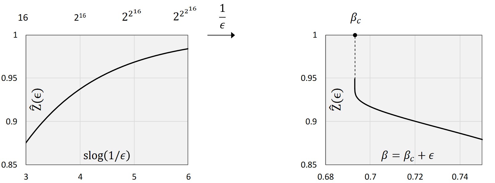
This continues (13) to any $\epsilon$. Although the continuation (6) of the super-logarithm to real values, and thus the continuation (17) of $\hat{Z}(\epsilon)$, is not unique, different continuations differ only by sub-leading orders in $\epsilon$. Thus, (17) is the leading singularity of the partition function $\hat{Z}(\epsilon)$ at the critical point. This partition function is plotted in fig. 3. It converges extremely slowly to $1$ as $\epsilon\rightarrow 0$, and is continuous but ”almost” discontinuous.

Armed with the results of section 5, let us now examine the phase transition for the counting machine near the critical point $\beta=\beta_{c}+\epsilon$ with $\beta_{c}=\ln 2,\epsilon\ll 1$. The free energy $F$ is:

$\displaystyle\hat{Z}(\beta)=e^{-\beta F}=\sum_{p}e^{-\beta l(p)}\ \ \Rightarrow\ \ F(\beta)=-{1\over\beta}\ln\hat{Z}(\beta)$

(18)

In our ensemble, the program length plays the role of the energy with expectation value

$\displaystyle\langle l\rangle_{\beta}=-\partial_{\beta}\ln\hat{Z}(\beta)$

(19)

The heat capacity is (using $T\partial_{T}=-\beta\partial_{\beta}$)

$$C(T)=-T{\partial^{2}F\over\partial T^{2}}\ \ \sim\ \ -\partial_{\beta}\ln\langle l\rangle\ \ +\ \ \text{higher orders in }\epsilon$$

According to the Ehrenfest classification, in a zeroth-order phase transition the free energy $F(T)$ is discontinuous at a critical point $T=T_{c}$. In a first-order transition, $F(T)$ is continuous but $\partial_{T}F(T)$ is discontinuous, the gap being the latent heat. In a second-order transition, $\partial_{T}F(T)$ is also continuous, but some higher-order derivative of $F(T)$ is discontinuous [8]. In our case,

$$\hat{Z}(\epsilon)=1-\lambda\cdot 2^{-\text{slog}_{2}(1/\epsilon)}\ =\ 1-\lambda\cdot 2^{-\lg^{-}(1/\epsilon)}\cdot\{\lg...\lg{(1/\epsilon)}\}^{-1}$$

where $\lambda\sim 0.186$, $\lg^{-}$ is the integer part of the super-logarithm and we have $\lg^{-}(1/\epsilon)$ iterations of the logarithm. Thus, in the limit $\epsilon\rightarrow 0$, we have, to leading order in $\epsilon$:

	$\displaystyle F(\epsilon)\ \$	$\displaystyle\propto$	$\displaystyle\ \ -\lambda\cdot 2^{-\lg^{-}(1/\epsilon)}\cdot\{\lg...\lg{(1/\epsilon)}\}^{-1}$
	$\displaystyle\langle l\rangle(\epsilon)\ \$	$\displaystyle\propto$	$\displaystyle\ \ [\ \epsilon\cdot\lg{1\over\epsilon}\cdot\lg\lg{1\over\epsilon}\cdot...\cdot(\lg...\lg{1\over\epsilon})^{2}\ ]^{-1}$		(20)
	$\displaystyle C(\epsilon)\ \$	$\displaystyle\propto$	$\displaystyle\ \ [\ \epsilon^{2}\cdot\lg{1\over\epsilon}\cdot\lg\lg{1\over\epsilon}\cdot...\cdot(\lg...\lg{1\over\epsilon})^{2}\ ]^{-1}$

$F(\epsilon)$ is finite at the critical point. It is continuous, but almost discontinuous. Thus, the phase transition is first-order, but almost zeroth order. We also see that the latent heat is infinite, meaning that the average program size $\langle l\rangle$ diverges at the critical point. The average size $N$ of the output strings also diverges, as $l\sim\lg N+\lg\lg N+...$

To put things into perspective, the age of the universe, as measured in Planck times, is $T_{u}\sim 2^{200}$. For $\epsilon<1/T_{u}$, one needs to consider input bit strings of length $l>T_{u}$, and therefore computation times $>T_{u}$, to compute $F$ and $\hat{Z}$ at $\beta=\beta_{c}+\epsilon$. The super-logarithm of $T_{u}$ is about 4.6, so for $\epsilon$ of order $2^{-200}$, $\hat{Z}$ is still about $0.76\%$ away from 1. To get a super-logarithm of 5, we would need a universe of age $2^{65^{\prime}536}$ Planck times. Even then, $\hat{Z}$ would still be $0.58\%$ away from 1. In this sense, the super-logarithmic singularity (the dashed line in fig. 2) is invisible at least for all bit string ensembles that can be computed in our universe, and $\text{slog}_{2}(1/\epsilon)$ is effectively cut off at $4.5-5$.

In the previous section, we have discussed the singularity of the partition function (7) near $\epsilon=0$ for the non-universal counting machine. How does it compare with the singularity for a universal Turing machine?

Since it is generally an undecidable question whether a given Turing machine halts for a given program, for a UTM the function $h_{l}$ in (7) and Chaitin’s $\Omega$ are not computable by any halting program. Neither is the singularity of $Z(\epsilon)$ at the critical point computable. In fact, $Z(\epsilon)$ converges towards $\Omega$ more slowly than any computable function.

To see this, let us slightly modify the last step of the counting machine of section 4: if, in the $i$-th step, $p_{m_{i-1}}=0$, the modified $T_{0}$ switches into a new mode: instead of writing $1^{n_{i-1}}$ on the work tape, it reads the next $\Sigma(n_{i-1})$ digits of the program $p$ from the program tape, where $\Sigma(n)$ is the busy-beaver function. The modified machine $\tilde{T}_{0}$ writes those digits on the work tape and then halts. Formula (11) thus gets replaced by

$$\tilde{Z}_{k}(\beta)=\sum_{n_{2},...,n_{k}}\sum_{N=0}^{2^{\Sigma(n_{k})}}e^{-\beta\cdot(6+n_{2}+...+n_{k}+\Sigma(n_{k}))}\sim\sum_{n_{2},...,n_{k}}2^{-(6+n_{2}+...+n_{k})}\cdot{1\over 2}\ e^{-\epsilon\cdot\Sigma(n_{k})}\ \ \$$

$\Sigma(n)$ is known to diverge faster than any computable function as $n\rightarrow\infty$. This implies that $\tilde{Z}(\epsilon)$ converges more slowly than any computable function to its critical value $1$ for the modified machine $\tilde{T}_{0}$. Now, any UTM $U$ simulates the modified machine $\tilde{T}_{0}$, if it is fed with all possible input programs. This implies that, for any UTM, $Z_{U}(\epsilon)$ converges more slowly than any computable function to its critical value $\Omega$.

The conclusions for UTM’s are thus similar as for the counting machine: first of all, at the critical point, the phase transition is first-order but almost zeroth-order, with a divergent latent heat (i.e. average program size). The average size of the output bit strings also diverges, as $U$ simulates $T_{0}$, among other machines. This divergent average program size is a pre-condition for a potential continuum limit of (2) at $\beta=\beta_{c}$, where very long bit strings might be described by continuous strings. This will be further discussed below.

Second, strictly speaking, $Z_{U}(\epsilon)$ for a UTM is continuous at $\epsilon=0$, but in practise, its behavior is indistinguishable from a discontinuity. This seems to make it impossible to get a better understanding of the Chaitin point (1) by first studying the ensemble (2) at low temperature (high $\beta$), and then taking the limit $\beta\rightarrow\beta_{c}$.

However, as in the case of the counting machine, this discontinuity is invisible in finite computation time. Thus, we can at least interpolate between the low-temperature phase and a ”real-world” version of the Chaitin point (1), in which the computation time is limited by the age $T_{u}$ of the universe. Alternatively, we could limit the length $L$ of the output bit strings $B$ to $L\leq T_{u}$ (roughly the diameter of the observable universe), and count only the shortest program that produces each $B$. As $B$ is produced by at least one program of size $L+O(1)$, namely ”print $B$”, this also limits the computation time. For most $B$, this amounts to replacing $K_{\beta}(B)$ by the Kolmogoroff complexity $K(B)$ in (4,5).

In this section, we discuss analogies and differences of the statistical-mechanical model (2) with quantum mechanics, both in the path integral- and the Hilbert space formulation. Our goal is to use these methods to better understand the approach to the critical point.

So far, we have only considered the input programs $p$ in (2), and not the bit strings $b$ that they produce on the work tape during the computation. Let us now rewrite (2) as a sum over paths in the space of configurations of the Turing machine. At any point in time, a configuration is uniquely specified by the 3-tuple [24]

$$S=\{b,s,k\},$$

where $b$ is the bit string on the work tape, $s$ is the state of the Turing machine, and $k$ is the position of the head. $k=1$ means that the head sits on the first non-blank bit of the work tape. We define ”program time” $\tau\in\{0,1,2,...,l\}$ as the position of the head on the read-only program tape. Let us represent a computation by a path $S(\tau)$ over the configurations at the time the $\tau$-th input bit is first read in, i.e, immediately before the path splits. The path ends at $\tau=l,b(l)=B,s(l)=$”Halt”, where $B$ is the output string.

Fig. 3 shows the computation paths and their first 15 output bit strings at the example of the counting machine. Fig. 3 can be thought of as an embedding of the tree graph of fig. 1 in configuration space. The bit string $b(\tau)$ is plotted on the horizontal axis, written as a decimal number $N$, except for the halting state ”H”, in which case $N$ denotes the length of the output bit string $1^{N}$. The states $s(\tau)$ and the position $k(\tau)$ of the work head are denoted by $s_{k}(\tau)$ and are plotted on the vertical axis (only certain configurations appear). The arrows show the direction of the computation; dashed arrows lead to configurations with $N>15$ and $s_{k}=5_{1}$. Black dots represent configurations before the paths split (”branchpoints”). The green/red bits shown along the example of the computation path leading to $B=11111_{2}$ ($N=5$) form the corresponding input program ”111010”.

It is instructive to compare with a particle on a Euclidean $N$-dimensional lattice with coordinates $\vec{x}$. The amplitude for the particle to go from point $\vec{a}$ to $\vec{b}$ is (see, e.g., [23]):

$\displaystyle G(\vec{a},\vec{b})$

$\displaystyle=$

$\displaystyle\sum_{l=0}^{\infty}N_{l}(\vec{a},\vec{b})\cdot\exp\{-\beta\cdot l\},$

(21)

where $N_{l}(\vec{a},\vec{b})$ is the number of paths $\vec{x}(\tau)$ (or ”world-lines”) of length $l$ on the lattice (measured in lattice spacings) that interpolate between $\vec{x}(0)=\vec{a}$ and $\vec{x}(l)=\vec{b}$. As $l\rightarrow\infty$, $N_{l}$ diverges as $\exp\{\beta_{c}\cdot l\}$, where the precise value of $\beta_{c}$ depends on the lattice. By setting

$$\beta=\beta_{c}+\epsilon m^{2}\ \ \text{as}\ \ \epsilon\rightarrow 0,$$

a continuum limit can be reached, where the model describes a lattice-independent relativistic particle of mass $m$ in $N$-dimensional Euclidean space with restored Poincaré symmetry. After a Wick rotation, this becomes a quantum mechanical particle in Minkowski space.

At least formally, the (high-dimensional) configuration space of the Turing machine is analogous to the lattice $\vec{x}$ of the particle, and the computation histories are analogous to the world lines $\vec{x}(\tau)$. The input bits on the program tape, which ”live” on the paths in fig. 3, correspond to the random variables $\vec{\eta}(\tau+1)=\vec{x}(\tau+1)-\vec{x}(\tau)$, which ”live” on the particle’s world line and describe its incremental movement on the lattice. Of course, a difference is that the computation of the Turing machine is irreversible, following the arrows in fig. 3, while the motion of the particle is reversible and symmetric: $G(\vec{a},\vec{b})=G(\vec{b},\vec{a})$.

Both for the particle and for the computation, the average length of the world lines diverges for $\epsilon\rightarrow 0$. The key question is what the computational analogue of the continuum limit of the relativistic quantum particle is. In trying to shed light on this, let us next discuss the corresponding Hilbert space in the case of the computation.

Using the classification of [24], let us begin by regarding the ensemble (2) as a probabilistic Turing machine. It acts on a Hilbert space of states, which are superpositions of the individual configurations $S$, each of them occurring with probability $p_{S}$:

$$|\Psi_{\tau}\rangle=\sum_{S}\ \psi_{S}(\tau)|S\rangle\ \ \ \text{with}\ \ \ \sum_{S}p_{S}=\sum_{S}|\psi_{S}|^{2}\leq 1,$$

(22)

Given a pure state $|S\rangle$ at time $\tau$, the next state at time $(\tau+1)$ is a superposition of the two possible successor configurations, each of which occurs with probability $e^{-\beta_{c}}\sim 1/2$. E.g., for the counting machine, if we define $l_{N}$ as in (8) and $\psi_{B}({\tau+1})=\psi_{B}(\tau)$ for $\tau\geq l$ (i.e., after the computation halts), then, in the limit $\tau\rightarrow\infty$, the output state converges to

$$|\Psi_{\infty}\rangle=\sum_{N=0}^{\infty}\psi_{N}|N\rangle\ \ \text{with}\ \ \ |N\rangle\equiv|1^{N},\text{Halt},1\rangle,\ \ \psi_{N}=2^{-l_{N}/2}\ \Rightarrow\ \sum_{N}|\psi_{N}|^{2}=1.$$

The evolution of $|\Psi_{\tau}\rangle$ from time $\tau$ to $\tau+1$ can be described by a transfer matrix $T$. This evolution is generally not reversible, and for a universal Turing machine not even probability is conserved due to non-halting programs (hence the $\leq$ sign in (22)). Thus, the transfer matrix $T$ is not unitary and the computation generates heat. However, $T$ can be extended such that the time evolution converges to a unitary one within the subspace $\hat{S}$ spanned by output states $|B\rangle$. E.g., an arbitrary phase $\delta_{B}$ can be added in the relation

$$\psi_{B}({\tau+1})=e^{i\delta_{B}}\psi_{B}(\tau)\ \ \text{for}\ \ \tau\geq l.$$

An example with applications to error-correction codes is Manin’s definition $\delta_{B}=K(B)$ [19]. It will be interesting to explore other applications for more general Transfer matrices $T=\exp\{i\tau H\}$, with a self-adjoint Hamiltonian $H$ acting on the space $\hat{S}$ of halting states. This turns the probabilistic Turing machine into a quantum Turing machine acting on $\hat{S}$.

In appendix A6, we consider the ensemble (4) for output strings $B_{L}$ of large but fixed length $L$. Using the above formalism, we discuss the ground state of the system for a (non-universal) toy model of a Turing machine, the ”kink machine”. At low-temperature ($\epsilon=\beta-\beta_{c}\gg 1/\lg L$), there is a degenerate, ordered ground state. As the temperature increases, kinks start to appear at $\epsilon\sim 1/\lg L$. They become dense at the critical point, thereby destroying the long-range order. A similar condensation of defects in spin models typically restores spontaneously broken symmetries and accompanies second-order phase transitions, where the models are described by universal continuum field theories. We must leave it for future work to examine whether analogous phenomena occur for a UTM.

To briefly summarize our results, let us denote programs that produce a given output bit string $B_{L}$ of length $L$ by $p(B_{L})$, and decompose our Gibbs ensemble (2) as

	$\displaystyle Z(\beta)$	$\displaystyle=$	$\displaystyle\sum_{L}Z_{L}(\beta)\ \ \ \text{with}$		(23)
	$\displaystyle Z_{L}(\beta)$	$\displaystyle=$	$\displaystyle\sum_{B_{L}}\ e^{-\beta\cdot K_{\beta}(B_{L})}\ \ ,\ \ e^{-\beta\cdot K_{\beta}(B_{L})}=\sum_{p(B_{L})}e^{-\beta\cdot l(p(B_{L}))}.$		(24)

We have shown that ensemble (23) has a first-order phase transition at the Chaitin point $\beta=\beta_{c}=\ln 2$. This phase transition is ”almost” zeroth-order, in the sense that the free energy is continuous but almost discontinuous: it converges to its critical value, namely Chaitin’s $\Omega$, more slowly than any computable function. However, for finite computation time and therefore limited $l$, this effective discontinuity is invisible, and one can smoothly interpolate between the classical limit $\beta\rightarrow\infty$ and the critical point $\beta=\beta_{c}$.

At the Chaitin point, we have shown that the latent heat (the average program size) and the average size of the output bit strings both diverge. This begs the question whether there is a continuum limit, in which long bit strings are described by continuum strings and the computation histories are represented by string world sheets. This must be decided in future work by adapting the tools of quantum mechanics and field theory to bit strings.

In section 9, we have taken a few preparatory steps in this direction. We have discussed analogies and differences with the continuum limit of a quantum particle on a lattice. We have also interpreted (23) as a probabilistic Turing machine and defined the analog of a Hilbert space of states. For the simplified toy model of appendix A6, we have examined the ground state of (24) for fixed length $L$. We have found a degenerate low-temperature ground state, whose long-range order is ”washed out” near the critical temperature by kinks, similarly as in second-order phase transitions in spin models.

While the sum over $L$ in (23) yields a first-order transition for $Z(\beta)$, this raises the question whether a universal Turing machine has a second-order transition for $Z_{L}(\beta)$, when $L$ is held fixed. As precedents of statistical mechanical models of dynamic size $L$ that have (i) zeroth- or first-order phase transitions when one sums over $L$, and (ii) second-order transitions for fixed $L$, consider the Ising model or the sine-Gordon model (referred to as ”matter”) on a random lattice [25, 26, 27]. In essence, the partition function is of the form

$$Z(\beta)=\sum_{L}\exp\{-\beta L\}\cdot Z_{\text{matter}}(L)\ \ ,\ \ L=\text{number of lattice sites}.$$

These models have zeroth-order phase transitions in $\beta$. However, as $\beta\rightarrow\beta_{c}$, $\langle L\rangle$ diverges, and the models have continuum limits, where the ”matter” undergoes second-order phase transitions on continuous random surfaces, whose area grows with $L$. These systems are described by two-dimensional field theories known as ”noncritical string theories”.

Why should we care about the order of the phase transition of the ensemble (2)? At second-order phase transitions, statistical mechanical models that are very complex on a microscopic scale often have simple, universal macroscopic descriptions in terms of continuum field theories. E.g., water and steam at a temperature of 374${}^{\text{o}}$C and a pressure of 218 atm is described by a scalar $\phi^{4}$ theory, which can be used to compute its critical exponents. At this critical point, almost all microscopic details become irrelevant. E.g., exactly the same critical exponents describe the second-order phase transition of CO₂, of simple lattice gas models, and of any other system in the same universality class.

Ensemble (23,24) certainly looks intractable on a microscopic scale: the action is higly nonlocal, and not even computable by any halting program. Our hope of better understanding Chaitin’s Omega therefore rests on the hypothesis that the ensemble has a tractable continuum limit at the Chaitin point, in the sense that it can be modelled by what could be called a ”logical quantum field theory” that is independent of the algorithmic details. We could then examine the ground state by approaching the critical temperature from below, as exemplified at the simple toy model of appendix A6.

Why do we want to better understand Chaitin’s Omega in the first place? It provides a fascinating link between information theory and statistical mechanics, for which many potential applications can be foreseen. Apart from the envisioned simulation of strings and the examination of their ground states, those include the analysis of heat generation in quantum Turing machines, the simulation of the evolution of species in terms of a Turing machine acting on DNA strings, or the generalization of the unitary time evolution of [19] to additional applications beyond error-correcting codes and Zipf’s law.

I would like to thank my brother Juergen Schmidhuber for arising my interest in information theory. The current work was inspired by his idea of the ”Great Programmer” [28]. This research is supported in part by grant no. CRSK-2 190659 from the Swiss National Science Foundation.

The appendix is organized as follows. A1 presents a Turing machine that contains only a work tape and no program tape. An example is given in A2. In A3, Chaitin’s definition of a Turing machine is recalled. Using the example of A2 as a building block, we realize the counting machine of section 4 in A4. A5 contains a supplementary argument to section 5. A6 constructs a computable transfer matrix/Hamiltonian for our ensemble (2).

References

- [1] G.J. Chaitin. A theory of program size formally identical to information theory. J. Assoc. Comput. Mach., 22:329–340, 1975
- [2] A.M. Turing. On computable numbers with an application to the Entscheidungsproblem. Proc. London Math. Soc., Ser. 2, 42:230–265, 1936. Correction, Ibid., 43:544–546, 1937
- [3] M. Li and P. Vitanyi, An Introduction to Kolmogorov Complexity and its Applications, 3rd edition, Springer Science+Business Media, 1993
- [4] K. Goedel, Ueber formal unentscheidbare Saetze der Principia Mathematica und verwandter Systeme I, Monatshefte fuer Mathematik und Physik 38: 173–98, 1931
- [5] Tadaki, K., 2002. A Generalization of Chaitin’s Halting Probability and Halting Self-Similar Sets. arXiv preprint nlin/0212001.
- [6] Calude, C.S. and Stay, M.A., 2006. Natural halting probabilities, partial randomness, and zeta functions. Information and Computation, 204(11), pp.1718-1739.
- [7] Baez, J.C. and Stay, M., 2010. Algorithmic thermodynamics. arXiv preprint arXiv:1010.2067.
- [8] J. Zinn-Justin, Quantum Field Theory and Critical Phenomena, Oxford University Press, 1989
- [9] M.M. Green, J.H. Schwarz and E. Witten, Superstring Theory vol. 1,2, Cambridge University Press, 1988
- [10] Tadaki K 2008 A statistical mechanical interpretation of algorithmic information theory, Local Proc. of Computability in Europe 2008 (CiE 2008) (University of Athens, Greece) p 425-434 June 15-20. Electronic Version: http://www.cs.swan.ac.uk/cie08/cie2008-local.pdf
- [11] Tadaki, K., 2012, February. Phase transition between unidirectionality and bidirectionality. In International Conference on Teaching and Computational Science (pp. 203-223). Springer, Berlin, Heidelberg.
- [12] Tadaki, K., 2014, July. Phase transition and strong predictability. In International Conference on Unconventional Computation and Natural Computation (pp. 340-352). Springer, Cham.
- [13] Kolmogorov, A.N., 1963. On tables of random numbers. Sankhyā: The Indian Journal of Statistics, Series A, pp.369-376.
- [14] Solomonoff, Ray J. ”A formal theory of inductive inference. Part I.” Information and control 7.1 (1964): 1-22. Part II.” Information and control 7.2 (1964): 224-254.
- [15] Levin, Leonid Anatolevich. ”Laws of information conservation (nongrowth) and aspects of the foundation of probability theory.” Problemy Peredachi Informatsii 10.3 (1974): 30-35.
- [16] Kolchinsky, Artemy, and David H. Wolpert. ”Thermodynamic costs of Turing machines.” Physical Review Research 2.3 (2020): 033312.
- [17] Landauer, R., 1961. Irreversibility and heat generation in the computing process. IBM journal of research and development, 5(3), pp.183-191.
- [18] Yuri I. Manin, 2008. Zipf’s law and avoidance of excessive synonymy. Cognitive Science, 32(7), pp.1075-1098.
- [19] Yuri I. Manin, Complexity vs energy: theory of computation and theoretical physics. Journal of Physics: Conference Series. Vol. 532. No. 1. IOP Publishing, 2014.
- [20] Yuri I. Manin, Physics in the World of Ideas: Complexity as Energy, ISCS 2014: Interdisciplinary Symposium on Complex Systems. Springer, Cham, 2015.
- [21] Cubitt, T.S., Perez-Garcia, D. and Wolf, M.M., 2015. Undecidability of the spectral gap. Nature, 528(7581), pp.207-211. Bausch, J., Cubitt, T., Lucia, A. and Perez-Garcia, D., 2018.
- [22] Undecidability of the spectral gap in one dimension. arXiv preprint arXiv:1810.01858.
- [23] Polyakov, A.M., Gauge Fields and Strings, chapter 9, contemporary concepts in physics vol. 3, harwood academic publishers, 1987
- [24] Fortnow, L., 2003. One complexity theorist’s view of quantum computing. Theoretical Computer Science, 292(3), pp.597-610.
- [25] D. Gross and A. Migdal, Nonperturbative Solution of the Ising Model on a Random Surface, Phys.Rev.Lett. 64, 1990
- [26] Moore, G., 1992. Gravitational phase transitions and the sine-Gordon model. arXiv preprint hep-th/9203061.
- [27] Christof Schmidhuber, Exactly marginal operators and running coupling constants in 2-D gravity, Nucl.Phys. B404, 1993
- [28] Juergen Schmidhuber, A Computer Scientist’s View of Life, the Universe, and Everything, in: Foundations of Computer Science: Potential - Theory - Cognition, Lecture Notes in Computer Science, ed. C. Freksa et al, Springer, 1997
- [29] Minsky, M.L., 1966. Size and structure of universal Turing machines using tag systems.
Appendix A: Review of Turing Machines