Two loop QCD amplitudes for di-pseudo scalar production in gluon fusionPreprint: IMSc/2019/09/08
Abstract
We compute the radiative corrections to the four-point amplitude in massless Quantum Chromodynamics (QCD) up to order in perturbation theory. We used the effective field theory that describes the coupling of pseudo-scalars to gluons and quarks directly, in the large top quark mass limit. Due to the CP odd nature of the pseudo-scalar Higgs boson, the computation involves careful treatment of chiral quantities in dimensional regularisation. The ultraviolet finite results are shown to be consistent with the universal infrared structure of QCD amplitudes. The infrared finite part of these amplitudes constitutes the important component of any next to next to leading order corrections to observables involving pair of pseudo-scalars at the Large Hadron Collider.
Keywords
QCD, Pseudo-scalar Higgs boson, Loop amplitudes, LHC1 Introduction
The discovery of Higgs boson of the standard model (SM) by ATLAS Aad:2012tfa and CMS Chatrchyan:2012xdj collaborations of the Large Hardron Collider (LHC) has not only put the SM on strong footing but also opened up a plethora of opportunities to investigate its properties and coupling to other SM particles. In certain beyond the SM (BSM) scenarios, one has enlarged Higgs sector, which allows more than one Higgs boson Fayet:1974pd; Fayet:1977yc; Dimopoulos:1981zb; Sakai:1981gr; Inoue:1982pi; Inoue:1983pp; Inoue:1982ej. For example, the minimal supersymmetric SM (MSSM), there are five Higgs bosons, out of which two of them are neutral scalars (h,H), one of them a pseudo scalar (A) and the remaining two are charged scalars (). The pseudo scalar Higgs boson which is CP odd could be as light as the discovered Higgs boson. Hence, a dedicated effort has been going on to determine the CP property of the discovered Higgs boson to identify with that of SM, which allows only CP even. This requires precise predictions for relevant observables for both scalar and pseudo scalar ones. In the case of SM Higgs boson, the production cross section has been computed in perturbative Quantum Chromodynamics (QCD) to unprecedented accuracy. This is possible, thanks to the fact that the top quark degrees of freedom can be integrated out. This results in an effective field theory (EFT) where scalar Higgs boson couples directly to the gluons even at leading order (LO). In the context of light Higgs boson in MSSM, unlike the SM one, the mass is calculable. In Martin:2007pg; Harlander:2008ju; Kant:2010tf, higher order radiative corrections to the mass are obtained to very good accuracy. For the pseudo scalar Higgs boson, there have been efforts to achieve precision in the predictions for production cross sections at the LHC. In Plehn:1996wb,first results on the production rate at NLO level in QCD for the pseudo scalar at the hadron collider appeared. This was done by keeping non-zero top quark mass. In Dawson:1998py EFT framework was set up by integrating out top quark fields, which opened up the possibility of obtaining observables beyond NLO level as there is a reduction of number of loops compared to those in the full theory. Unlike the case of CP even Higgs boson, inclusive cross section for the production of pseudo scalar Higgs is known Harlander:2002vv; Anastasiou:2002wq; Ravindran:2003um only up to next-to-next-to leading order (NNLO) in pQCD. For N3LO predictions, one requires three loop virtual amplitudes and real emission contributions. The computation of virtual corrections is technically challenging Ahmed:2015qpa as pseudo scalar Higgs boson couples to SM fields through two composite operators that mix under renormalisation. In addition, these operators involve Levi-Civita tensor and which are hard to define in dimensional regularisation. The three loop form factor thus obtained was later combined with appropriate soft distribution function Ravindran:2005vv; Ravindran:2006cg; Ahmed:2014cla and mass factorisation kernels to obtain soft plus virtual contribution at N3LO in QCD Ahmed:2015qda. Later, the process dependent resummation constants from the three loop form factors were used to perform threshold resummation in Ahmed:2016otz and also make approximate prediction at N3LO level. This was possible due to the similarity of the interaction vertices of scalar and pseudo scalar Higgs bosons with the gluons.
Recently, there have been a surge of interest to study the production of pair of Higgs bosons to determine Higgs self coupling, whose strength is a prediction of the SM, if the mass of the Higgs boson is known. Measurement of this coupling will provide an independent test on nature of the Higgs boson. The gluon gluon fusion subprocess producing pair of Higgs bosons through a heavy quark loop Glover:1987nx; Plehn:1996wb is the dominant one at the LHC, however the cross section is only few tens of fb, making it very difficult to observe. QCD corrections not only increase the cross section but also stabilise the predictions against renormalisation , and factorisation scales. NLO QCD corrections Dawson:1998py and later on the top quark mass effects are systematically taken into account in Grigo:2013rya; Frederix:2014hta; Maltoni:2014eza; Degrassi:2016vss; Borowka:2016ehy; Borowka:2016ypz. Beyond NLO, an EFT where top quark degrees of freedom are integrated out is used. At present, production of pair of Higgs bosons in EFT is known to N3LO level Chen:2019lzz, for NLO, NNLO, see deFlorian:2013uza; Grigo:2015dia; deFlorian:2013jea; Grigo:2013rya; Frederix:2014hta; Maltoni:2014eza; Degrassi:2016vss; Borowka:2016ehy; Borowka:2016ypz. All the two loop virtual amplitudes for that are required for the N3LO cross section for the di-Higgs production were obtained in Banerjee:2018lfq. The production of di-Higgs bosons through bottom quark annihilation was obtained up to NNLO level in H:2018hqz. In Li:2013flc; Maierhofer:2013sha; deFlorian:2015moa, the fully differential results at NNLO level are presented. While, there have been flurry of activities in the context of scalar Higgs boson, very little is known for the production of pair of pseudo scalar Higgs bosons at the LHC so far. In Dawson:1998py, LO contribution keeping finite top mass and NLO contributions using EFT framework where top quark degrees of freedom are integrated out have been obtained. Like the production of single pseudo scalar Higgs boson, pair production is also important to understand the nature of the extended Higgs sector. In order to reduce the theoretical uncertainties, it is important to have QCD radiative corrections under control. Due to EFT, it is now possible to go beyond NLO with available tools to make precise as well as stable predictions with respect to the unphysical scales. At NNLO level, we require two loop virtual, one loop single real emission and double real emission amplitudes. In this article, as a first step towards obtaining going beyond NLO QCD corrections, we compute all the one and two loop amplitudes that can contribute to the pure virtual part of the cross section in dimensional regularisation and perform ultraviolet (UV) renormalisation to obtain UV finite results.
The paper is organised as follows: in section-2, we describe how two loop virtual amplitudes are computed. In particular, we introduce the effective Lagrangian, the relevant kinematics, describe how projector method can be applied to obtain the scalar parts of the amplitudes, the subtleties involved in defining the Levi-Civita tensor and in dimensional regularisation, ultraviolet renormalisation of strong coupling, over all renormalisations for the composite operators and finite renormalisation for the . In section-3, computation of the amplitudes and their infrared (IR) structure are briefly discussed. In section-4, we summarise our results and conclude.
2 Theoretical framework
2.1 Effective Lagrangian
We work with the effective Lagrangian Chetyrkin:1998mw that describes the interaction of the pseudo-scalar field with the gauge field and the fermion :
| (1) |
The pseudo-scalar gluonic () and the light quark () operators are defined as
| (2) |
where is the SU(3) structure constant and is the Levi-Civita tensor. The pseudo-scalar fermionic operator is the derivative of the flavour singlet axial vector current
| (3) |
The effective Lagrangian is obtained after integrating out the top quark fields in the large top mass limit. Hence, the corresponding Wilson coefficients CG and CJ depend on the mass of the top quark . As a result of the Adler-Bardeen theorem Adler:1969gk, there is no QCD correction to CG beyond one-loop level. On the other hand, CJ begins only at second-order in the strong coupling constant . The Wilsons coefficients are given by
| (4) | ||||
| (5) |
where is the Fermi constant, – the ratio of the vacuum expectation values of the two Higgs doublets, in a model where the CP is not spontaneously broken. is the quadratic Casimir in the fundamental representation of QCD and is the renormalisation scale at which is renormalised.
We use the effective lagrangian 1 to obtain amplitudes for the production of pair of pseudo-scalar Higgs bosons of mass up to two loop level in perturbative QCD. We restrict ourselves to the dominant gluon fusion subprocess:
| (6) |
where and are the momenta of the incoming gluons, and and are the momenta of the outgoing pseudo-scalar Higgs bosons, . The Mandelstam variables for the above process are given by
| (7) |
which satisfy . It is convenient to express these amplitudes in terms of the dimensionless variables , and as
| (8) |
which lead to the constraint .
As in the case of di-Higgs production amplitude via gluon fusion Glover:1987nx, the di-pseudo scalar production amplitude, can also be decomposed in terms of two second rank Lorentz tensors (), as follows:
| (9) |
where are the polarisation vectors of the initial state gluons. The Lorentz scalar functions , are independently gauge invariant. indicates that there is no colour flow from initial to final state. The second rank tensors are given by
| (10) | |||||
with is the transverse momentum square of the pseudo-scalar Higgs boson expressed in terms of the Mandelstam variables. The tensor depends only on the initial state momenta . Using momentum conservation, it can be seen that is symmetric under the interchange of the two pseudo-scalar Higgs momenta. The scalar functions can be obtained from , by using appropriate -dimensional projectors with , respectively and the projectors are given by:
| (12) |
where corresponds to the colour group.
In the following, we briefly discuss on the type of Feynman diagrams that contribute up to order in QCD. To evaluate the 4-point amplitude to any order in , one needs to calculate the contributing diagrams to that particular order and evaluate the scalar functions , using the projectors , . Using the effective Lagrangian eq.(̃1), the higher order corrections to amplitude are calculated in massless QCD. There are two types of diagrams that contribute to this process. We classify them as type-I and type-II. The form factor type diagrams where a pair of gluons annihilate to a single A, which branches into a pair of As belong to type-I and type-II contains t and u channel diagrams where each A is coupled to pair of gluons, or to quarks. In type-I, we have two classes of diagrams: type-Ia (fig. 1 left panel) which contains only four point effective vertex and type-Ib (fig. 1 right panel) containing both and vertices. These diagrams contribute at tree level () and we need to calculate them to i.e., up to 3-loop order. Since these diagrams are related to form factors of between gluons states and between quark and gluon states, we can readily obtain them from Baikov:2009bg; Gehrmann:2010ue; Ahmed:2015qpa.
The type-II diagrams consist of (a) two effective vertex (fig. 2) and (b) one effective vertex and one effective vertex as shown in fig. 3. Due to the axial anomaly, the pseudo-scalar operator for the gluonic field strength mixes with the divergence of the singlet axial vector current. The effective vertex is proportional to the Wilson coefficient (eq. 4) which is constrained to order due to the Alder-Bardeen Theorem. The tree level diagram in type-IIa (fig. 2) starts at order and each higher loop order adds an order . The effective vertex is proportional to , the Wilson coefficient (eq. 5) which starts at order . The type-IIb diagrams (fig. 3) which consist of one effective vertex and one effective vertex start at one loop level at .
Since, type-I diagrams are known to required order in , the results presented in this paper will mainly include the type-II amplitudes up to two loops in massless perturbative QCD i.e. order . We use dimensional regularisation () to regularise both UV and IR singularities which appear as poles in in the UV, soft and collinear regions. Since we will have to deal with the Levi-Civita tensor in operator and in operator, both of which are constructs inherently in 4-dimensions, a consistent method to deal with them in dimensions is essential. We discuss the details of a consistent and practical prescription to go over to and its implications in the next section. Hence, the scalar amplitudes can be written as a sum of amplitudes resulting from types-I and II diagrams as
| (13) |
and in the following we concentrate only on .
2.2 within dimensional regularisation
Due to the axial anomaly, the pseudo-scalar gluonic operator is related to the divergence of the axial vector current . Computation of higher order corrections with chiral quantities, involve inherently dimensional objects like and the Levi-Civita tensor , and this warrants a prescription in going away from 4-dimension i.e. . There exist several prescriptions to deal with in dimensional regularisation tHooft:1972tcz; Korner:1991sx. In multi-loop computations that use dimensional regularisation, we use the self-consistent prescription for that was proposed by ’t Hooft and Veltman tHooft:1972tcz. In this prescription, one defines as
| (14) |
where Levi-Civita tensor is purely 4-dimensional, while the Lorentz indices on the are in dimensions. To maintain the anti-commuting nature of with -dimensional , the symmetrical form of the axial current has to be used
| (15) |
this is in concurrence with the above definition of in eq. 14, and will lead to
| (16) |
The and operators now take the form
| (17) |
Contraction of two Levi-Civita tensors that result from either operator or the mixing of and operators is given by
| (18) |
the Lorentz indices in this determinant, could now be considered as -dimensional and the consequence would be, addition of only the inessential terms to the renormalisated quantity Larin:1993tq. This prescription though is not without consequence– a finite renormalisation of the axial vector current Larin:1991tj is required in order to fulfill the chiral Ward identities and the Adler-Bardeen theorem. This will be discussed further in the next section.
2.3 UV renormalisation, operator renormalization and mixing
In dimensional regularisation with , the bare strong coupling constant denoted by is related to its renormalized coupling by
| (19) |
with with the Euler-Mascheroni constant and is the scale introduced to keep the strong coupling constant dimensionless in space-time dimensions. The renormalisation constant Tarasov:1980au is given by
| (20) |
up to . are the coefficients of the QCD function and are given by Tarasov:1980au
| (21) |
where is the number of flavors and . As we work in an effective theory obtained after integrating out the top quark fields in the large top quark mass limit, . The Casimirs of SU(N) are given by and :
| (22) |
For type-I diagrams which begin to contribute at LO, the up to order will be needed while for type-II diagrams, one order lower is sufficient.
Apart from the renormalisation of strong coupling in the massless QCD, the amplitudes require the renormalisation of vertices resulting from the composite operators and of the effective Lagrangian eq. (1). The renormalised operators are denoted by parenthesis, while the bare quantities without the parenthesis.
The renormalisation of is related to the renormalisation of the singlet axial vector current which needs the standard overall UV renormalisation constant and a finite renormalisation constant . The later is necessary in dimensional regularisation in order to ensure the nature of operator relation resulting from axial anomaly Adler:1969er
| (23) |
which is true in Pauli-Villars, a 4-dimensional regularisation. To preserve eq. 23 in dimensions, the multiplicative finite renormalisation constant is required. The bare operator is renormalised multiplicatively, exactly in the same way as the singlet axial vector current , through
| (24) |
whereas the bare pseudo-scalar gluon operator mixes with fermionic operator under the renormalisation through
| (25) |
with the corresponding renormalisation constants and . Combining the above two equations in a matrix form, we have
| (26) |
| (27) |
where to all orders in perturbation theory and . The renormalisation constants required for above equation are available up to Larin:1993tq, Zoller:2013ixa which was computed using OPE. For earlier works on this, see Kataev:1981aw; Kataev:1981gr. Using a completely different method the same quantities were calculated by some of us Ahmed:2015qpa and found to be in full agreement. The UV renormalisation constant of the singlet axial vector current in the scheme is
| (28) |
and the finite renormalisation constant is
| (29) |
The renormalisation constants for and operators up to two loops are given by
| (30) |
The matrix element that would contribute to the amplitude can be obtained via the insertion of two renormalised operators (eq. 25) and (eq. 24) for each , which would involve the following operator insertion between gluon states:
| (31) |
The above operator renormalisation constants (eq. 2.3) and the strong coupling renormalisation constant (eq. 20) would take care of the UV renormalisation. The gluonic operator couples to gluons at LO () and the fermionic operator couples to quarks at LO (). The basic matrix elements that have to be evaluated diagrammatically involve the following bare operators combination: , and . The starts to contribute at tree level at , begins to contribute at one-loop level and at while starts to contribute at . Here we compute amplitude to order and hence the contributing terms are from calculated up to two-loops and the combination from one-loop. We need the following renormalised operator and which is given by
| (32) |
Sandwiching and between gluon states and using eq. (2.3), we obtain up to two loops:
| (33) |
where and , with that contribute to the type-II diagrams. , and do not contribute in our case as they are of order higher than when combined with their respective Wilson coefficients. Finally, can be expressed in powers of renormalised as
| (34) |
The coefficients can be related to using eq. 20 and eq. 2.3. Expanding the renormalisation constants in eq. 2.3 as
| (35) |
we find
| (36) | |||||
Similarly for , we find
| (37) |
where
| (38) |
We find that the UV singularities that appear at one-loop and two-loop levels can be taken care of by the coupling constant renormalisation and operator renormalisation . At this point we would like to stress that there could be additional contact terms required as a result of the behaviour of product of operators or at short distances. As shown in Zoller:2013ixa, we find that there are no contact terms as a result of these product of operators at short distances. For earlier works on this, see Kataev:1981aw; Kataev:1981gr.
3 Calculational details
3.1 Calculation of the Amplitude
Our task of computing the amplitude has reduced to the type-II diagrams up to . This involves diagrams with two effective vertices, up to two-loop level in QCD (Type-IIa) and diagrams with one effective vertex and one effective vertex which involves terms up to one loop in QCD (Type-IIb). Diagrams involving two effective vertex start at and are not considered here. Applying the projectors on the amplitudes, we extract the scalar coefficients with at every order in the perturbation.
All the tree level, one loop and two loop Feynman diagrams in massless QCD are generated using QGRAF Nogueira:1991ex where additional vertices resulting from effective lagrangian eq. (1) are incorporated. There are two tree level diagrams, 35 one-loop diagrams and 789 two-loop diagrams of type-IIa. For type-IIb which involves effective quark and gluon couplings to pseudo-scalar Higgs, there are no tree level diagrams but 8 diagrams that contribute at one-loop which suffices to generate diagrams up to . The raw QGRAF output is converted with the help of in-house codes based on FORM Vermaseren:2000nd to include appropriate Feynman rules and to perform trace of Dirac matrices, contraction of Lorentz indices and colour indices. At this stage, we encounter huge number of one and scalar 2-loop Feynman integrals, which contain a set of propagator denominators and a combination of scalar products between loop momenta and independent external momenta. These Feynman integrals can be classified in terms of propagator denominators, that they contain. It is hence important to identify the momentum shifts that are required to express each of these diagrams in terms of a standard set of propagators called auxiliary topology. We use REDUZE2 package vonManteuffel:2012np to achieve this. The auxiliary topologies needed for the present case are same as those found in vector boson pair production Gehrmann:2013cxs; Gehrmann:2014bfa at two loops.
As expected these large number of scalar integrals are not all independent. To establish the relations, some properties of the Feynman integrals in dimensional regularisation are used. Exploiting the fact that, the total derivative with respect to any loop momenta of these integrals, evaluates to a surface term, which vanishes, leads to integration-by-parts (IBP) identities Tkachov:1981wb; Chetyrkin:1981qh. In addition, the fact that all integrals are Lorentz scalars, gives rise to Lorentz invariance (LI) identities Gehrmann:1999as. As a result, these integrals can in turn be expressed in terms of a much smaller set of integrals which are irreducible and appropriately called master integrals (MI). Several automated computer algebra packages are available Anastasiou:2004vj; Smirnov:2008iw; Studerus:2009ye; vonManteuffel:2012np; Lee:2013mka that use the Laporta algorithm Laporta:2001dd to reduce these Feynman integrals to the MIs. We have used the Mathematica based package LiteRed Lee:2013mka to perform the reductions of all the integrals to MIs. At one-loop, there are 10 MIs, while at two-loop the number is 149. These two-loop MIs are the same as two-loop four-point functions with two equal mass external legs. The analytical result for the each MI in terms of Laurent series expansion in is given in Gehrmann:2013cxs; Gehrmann:2014bfa.
At this stage, the renormalisation of the strong coupling constant and of the operators and , described in section 2.3, removes all the UV singularities. The singularities that still remain are purely of infrared origin and the next section is devoted to it.
3.2 Infrared factorization
The UV finite amplitudes that we have computed contain only divergences of infrared origin, which appear as poles in the dimensional regularization parameter . They are expected to cancel against real emission diagrams for the IR safe observables. While these singularities disappear in the physical observables, the amplitudes beyond leading order show a very rich universal structure in the IR. In Catani:1998bh, Catani predicted the IR poles of two-loop n-point UV finite amplitudes in terms of certain universal IR anomalous dimensions. Later, in Sterman:2002qn, factorization and resummation properties of QCD amplitudes were used to understand the IR structure and subsequently the attempts were made to predict the structure of IR poles beyond two loops in Becher:2009cu; Gardi:2009qi. Following Catani:1998bh, we obtain
| (39) |
where are the IR singularity operators given by
| (40) | ||||
| (41) |
with
| (42) | |||||
| (43) | |||||
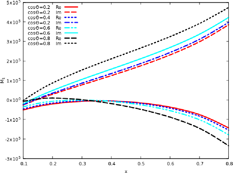
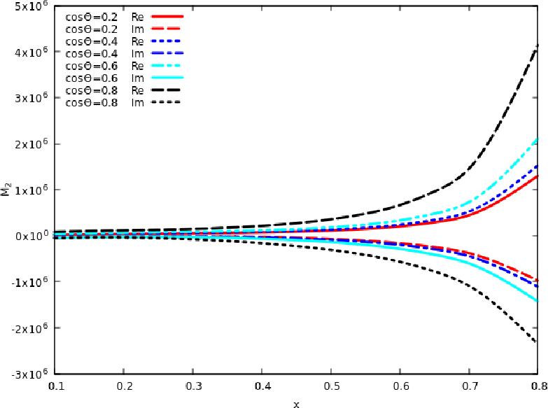
At one loop level, it is straight forward to show analytically that the IR poles are in agreement with the predictions. For the two loop case a fully analytical comparison was possible only for poles with . However, due to the large file size for the pole term, we made a comparison only at the numerical level. We found full agreement with the predictions of Catani up to two loop level for all the IR poles. Having obtained the IR pole cancellations, the finite part defined in eq. 3.2 can be extracted by subtracting the IR poles. Expressions for the finite part are too large to be presented here, however, they are being provided as ancillary files. The finite part of the amplitude corresponding to the projectors 1 and 2 as a function of for different values of is plotted normalising appropriately, in fig. 4.
The finite part in eq. (33) starts at one loop and contributes at order when combined with their respective Wilson coefficients. For projector 1 and 2, we have
| (44) | |||||
| (45) |
4 Discussion and Conclusions
In this paper, we have presented the two loop virtual amplitudes that are relevant for studying
production of pair of pseudo-scalar Higgs bosons in gluon fusion subprocess at the LHC.
This is the dominant sub process that is sensitive to its self coupling. We have done this
computation in the EFT where top quark degrees of freedom is integrated out.
In the EFT, the pseudo-scalar Higgs boson directly couples to gluons and light quarks through
two local composite operators and respectively with the strengths proportional to
Wilson coefficients that are calculable in perturbative QCD. We used dimensional regularisation
to regulate both UV and IR divergences. The composite operators being CP odd, contain Levi-Civita
tensor and which are inherently four dimensional objects. Hence, a careful treatment was
needed to deal with them in -dimensions. We followed the prescription advocated by Larin.
This requires additional renormalisation for the singlet axial vector current up to two loops.
In addition, Larin’s prescription requires finite renormalistion constant for
singlet axial current and is also available.
Note that the composite operators mix under UV rerenormalistion.
The corresponding renormalisation constants are already known and we use them to obtain UV finite
two loop amplitudes.
Unlike the amplitudes involving pair of Higgs bosons, we do not need any UV contact counter terms.
The UV finite amplitudes thus obtained contain IR divergences
due to the presence of massless partons in QCD. We found that these IR poles are in agreement with the predictions
by Catani and it provides a test on the correctness of the computation. Our results provide
one of the important components relevant for studies related to
production of pair of pseudo-scalar Higgs bosons at the LHC up to order .
Acknowledgement: We would like to acknowledge the support of the CNRS LIA (Laboratoire International Associe’) THEP (Theoretical High Energy Physics) and the INFRE-HEPNET (IndoFrench Network on High Energy Physics) of CEFIPRA/IFCPAR (Indo-French Centre for the Promotion of Advanced Research). We thank T. Gehrmann for providing us the master integrals and Roman Lee for his help with LiteRed. We would like to thank Prasanna K Dhani for discussions. AB would like to thank Pooja Mukherjee and A.H. Ajjath for their guidance. She would also like to thank her colleagues in the Theory division for their help.
References
- (1) ATLAS collaboration, G. Aad et al., Observation of a new particle in the search for the Standard Model Higgs boson with the ATLAS detector at the LHC, Phys. Lett. B716 (2012) 1 [1207.7214].
- (2) CMS collaboration, S. Chatrchyan et al., Observation of a New Boson at a Mass of 125 GeV with the CMS Experiment at the LHC, Phys. Lett. B716 (2012) 30 [1207.7235].
- (3) P. Fayet, Supergauge Invariant Extension of the Higgs Mechanism and a Model for the electron and Its Neutrino, Nucl. Phys. B90 (1975) 104.
- (4) P. Fayet, Spontaneously Broken Supersymmetric Theories of Weak, Electromagnetic and Strong Interactions, Phys. Lett. 69B (1977) 489.
- (5) S. Dimopoulos and H. Georgi, Softly Broken Supersymmetry and SU(5), Nucl. Phys. B193 (1981) 150.
- (6) N. Sakai, Naturalness in Supersymmetric Guts, Z. Phys. C11 (1981) 153.
- (7) K. Inoue, A. Kakuto, H. Komatsu and S. Takeshita, Aspects of Grand Unified Models with Softly Broken Supersymmetry, Prog. Theor. Phys. 68 (1982) 927.
- (8) K. Inoue, A. Kakuto, H. Komatsu and S. Takeshita, Renormalization of Supersymmetry Breaking Parameters Revisited, Prog. Theor. Phys. 71 (1984) 413.
- (9) K. Inoue, A. Kakuto, H. Komatsu and S. Takeshita, Low-Energy Parameters and Particle Masses in a Supersymmetric Grand Unified Model, Prog. Theor. Phys. 67 (1982) 1889.
- (10) S. P. Martin, Three-loop corrections to the lightest Higgs scalar boson mass in supersymmetry, Phys. Rev. D75 (2007) 055005 [hep-ph/0701051].
- (11) R. V. Harlander, P. Kant, L. Mihaila and M. Steinhauser, Higgs boson mass in supersymmetry to three loops, Phys. Rev. Lett. 100 (2008) 191602 [0803.0672].
- (12) P. Kant, R. V. Harlander, L. Mihaila and M. Steinhauser, Light MSSM Higgs boson mass to three-loop accuracy, JHEP 08 (2010) 104 [1005.5709].
- (13) T. Plehn, M. Spira and P. M. Zerwas, Pair production of neutral Higgs particles in gluon-gluon collisions, Nucl. Phys. B479 (1996) 46 [hep-ph/9603205].
- (14) S. Dawson, S. Dittmaier and M. Spira, Neutral Higgs boson pair production at hadron colliders: QCD corrections, Phys. Rev. D58 (1998) 115012 [hep-ph/9805244].
- (15) R. V. Harlander and W. B. Kilgore, Production of a pseudoscalar Higgs boson at hadron colliders at next-to-next-to leading order, JHEP 10 (2002) 017 [hep-ph/0208096].
- (16) C. Anastasiou and K. Melnikov, Pseudoscalar Higgs boson production at hadron colliders in NNLO QCD, Phys. Rev. D67 (2003) 037501 [hep-ph/0208115].
- (17) V. Ravindran, J. Smith and W. L. van Neerven, NNLO corrections to the total cross-section for Higgs boson production in hadron hadron collisions, Nucl. Phys. B665 (2003) 325 [hep-ph/0302135].
- (18) T. Ahmed, T. Gehrmann, P. Mathews, N. Rana and V. Ravindran, Pseudo-scalar Form Factors at Three Loops in QCD, JHEP 11 (2015) 169 [1510.01715].
- (19) V. Ravindran, On Sudakov and soft resummations in QCD, Nucl. Phys. B746 (2006) 58 [hep-ph/0512249].
- (20) V. Ravindran, Higher-order threshold effects to inclusive processes in QCD, Nucl. Phys. B752 (2006) 173 [hep-ph/0603041].
- (21) T. Ahmed, M. Mahakhud, N. Rana and V. Ravindran, Drell-Yan Production at Threshold to Third Order in QCD, Phys. Rev. Lett. 113 (2014) 112002 [1404.0366].
- (22) T. Ahmed, M. C. Kumar, P. Mathews, N. Rana and V. Ravindran, Pseudo-scalar Higgs boson production at threshold N3 LO and N3 LL QCD, Eur. Phys. J. C76 (2016) 355 [1510.02235].
- (23) T. Ahmed, M. Bonvini, M. C. Kumar, P. Mathews, N. Rana, V. Ravindran et al., Pseudo-scalar Higgs boson production at N3 LO +N3 LL ′, Eur. Phys. J. C76 (2016) 663 [1606.00837].
- (24) E. W. N. Glover and J. J. van der Bij, HIGGS BOSON PAIR PRODUCTION VIA GLUON FUSION, Nucl. Phys. B309 (1988) 282.
- (25) J. Grigo, J. Hoff, K. Melnikov and M. Steinhauser, On the Higgs boson pair production at the LHC, Nucl. Phys. B875 (2013) 1 [1305.7340].
- (26) R. Frederix, S. Frixione, V. Hirschi, F. Maltoni, O. Mattelaer, P. Torrielli et al., Higgs pair production at the LHC with NLO and parton-shower effects, Phys. Lett. B732 (2014) 142 [1401.7340].
- (27) F. Maltoni, E. Vryonidou and M. Zaro, Top-quark mass effects in double and triple Higgs production in gluon-gluon fusion at NLO, JHEP 11 (2014) 079 [1408.6542].
- (28) G. Degrassi, P. P. Giardino and R. Gröber, On the two-loop virtual QCD corrections to Higgs boson pair production in the Standard Model, Eur. Phys. J. C76 (2016) 411 [1603.00385].
- (29) S. Borowka, N. Greiner, G. Heinrich, S. P. Jones, M. Kerner, J. Schlenk et al., Higgs Boson Pair Production in Gluon Fusion at Next-to-Leading Order with Full Top-Quark Mass Dependence, Phys. Rev. Lett. 117 (2016) 012001 [1604.06447].
- (30) S. Borowka, N. Greiner, G. Heinrich, S. P. Jones, M. Kerner, J. Schlenk et al., Full top quark mass dependence in Higgs boson pair production at NLO, JHEP 10 (2016) 107 [1608.04798].
- (31) L.-B. Chen, H. T. Li, H.-S. Shao and J. Wang, Higgs boson pair production via gluon fusion at N3LO in QCD, 1909.06808.
- (32) D. de Florian and J. Mazzitelli, Two-loop virtual corrections to Higgs pair production, Phys. Lett. B724 (2013) 306 [1305.5206].
- (33) J. Grigo, J. Hoff and M. Steinhauser, Higgs boson pair production: top quark mass effects at NLO and NNLO, Nucl. Phys. B900 (2015) 412 [1508.00909].
- (34) D. de Florian and J. Mazzitelli, Higgs Boson Pair Production at Next-to-Next-to-Leading Order in QCD, Phys. Rev. Lett. 111 (2013) 201801 [1309.6594].
- (35) P. Banerjee, S. Borowka, P. K. Dhani, T. Gehrmann and V. Ravindran, Two-loop massless QCD corrections to the four-point amplitude, JHEP 11 (2018) 130 [1809.05388].
- (36) A. H. Ajjath, P. Banerjee, A. Chakraborty, P. K. Dhani, P. Mukherjee, N. Rana et al., Higgs pair production from bottom quark annihilation to NNLO in QCD, JHEP 05 (2019) 030 [1811.01853].
- (37) Q. Li, Q.-S. Yan and X. Zhao, Higgs Pair Production: Improved Description by Matrix Element Matching, Phys. Rev. D89 (2014) 033015 [1312.3830].
- (38) P. Maierhöfer and A. Papaefstathiou, Higgs Boson pair production merged to one jet, JHEP 03 (2014) 126 [1401.0007].
- (39) D. de Florian and J. Mazzitelli, Higgs pair production at next-to-next-to-leading logarithmic accuracy at the LHC, JHEP 09 (2015) 053 [1505.07122].
- (40) K. G. Chetyrkin, B. A. Kniehl, M. Steinhauser and W. A. Bardeen, Effective QCD interactions of CP odd Higgs bosons at three loops, Nucl. Phys. B535 (1998) 3 [hep-ph/9807241].
- (41) S. L. Adler, Axial vector vertex in spinor electrodynamics, Phys. Rev. 177 (1969) 2426.
- (42) P. A. Baikov, K. G. Chetyrkin, A. V. Smirnov, V. A. Smirnov and M. Steinhauser, Quark and gluon form factors to three loops, Phys. Rev. Lett. 102 (2009) 212002 [0902.3519].
- (43) T. Gehrmann, E. W. N. Glover, T. Huber, N. Ikizlerli and C. Studerus, Calculation of the quark and gluon form factors to three loops in QCD, JHEP 06 (2010) 094 [1004.3653].
- (44) G. ’t Hooft and M. J. G. Veltman, Regularization and Renormalization of Gauge Fields, Nucl. Phys. B44 (1972) 189.
- (45) J. G. Korner, D. Kreimer and K. Schilcher, A Practicable gamma(5) scheme in dimensional regularization, Z. Phys. C54 (1992) 503.
- (46) S. A. Larin, The Renormalization of the axial anomaly in dimensional regularization, Phys. Lett. B303 (1993) 113 [hep-ph/9302240].
- (47) S. A. Larin and J. A. M. Vermaseren, The alpha-s**3 corrections to the Bjorken sum rule for polarized electroproduction and to the Gross-Llewellyn Smith sum rule, Phys. Lett. B259 (1991) 345.
- (48) O. V. Tarasov, A. A. Vladimirov and A. Yu. Zharkov, The Gell-Mann-Low Function of QCD in the Three Loop Approximation, Phys. Lett. 93B (1980) 429.
- (49) S. L. Adler and W. A. Bardeen, Absence of higher order corrections in the anomalous axial vector divergence equation, Phys. Rev. 182 (1969) 1517.
- (50) M. F. Zoller, OPE of the pseudoscalar gluonium correlator in massless QCD to three-loop order, JHEP 07 (2013) 040 [1304.2232].
- (51) A. L. Kataev, N. V. Krasnikov and A. A. Pivovarov, The Connection Between the Scales of the Gluon and Quark Worlds in Perturbative QCD, Phys. Lett. 107B (1981) 115.
- (52) A. L. Kataev, N. V. Krasnikov and A. A. Pivovarov, Two Loop Calculations for the Propagators of Gluonic Currents, Nucl. Phys. B198 (1982) 508 [hep-ph/9612326].
- (53) P. Nogueira, Automatic Feynman graph generation, J. Comput. Phys. 105 (1993) 279.
- (54) J. A. M. Vermaseren, New features of FORM, math-ph/0010025.
- (55) A. von Manteuffel and C. Studerus, Reduze 2 - Distributed Feynman Integral Reduction, 1201.4330.
- (56) T. Gehrmann, L. Tancredi and E. Weihs, Two-loop master integrals for : the planar topologies, JHEP 08 (2013) 070 [1306.6344].
- (57) T. Gehrmann, A. von Manteuffel, L. Tancredi and E. Weihs, The two-loop master integrals for , JHEP 06 (2014) 032 [1404.4853].
- (58) F. V. Tkachov, A Theorem on Analytical Calculability of Four Loop Renormalization Group Functions, Phys. Lett. 100B (1981) 65.
- (59) K. G. Chetyrkin and F. V. Tkachov, Integration by Parts: The Algorithm to Calculate beta Functions in 4 Loops, Nucl. Phys. B192 (1981) 159.
- (60) T. Gehrmann and E. Remiddi, Differential equations for two loop four point functions, Nucl. Phys. B580 (2000) 485 [hep-ph/9912329].
- (61) C. Anastasiou and A. Lazopoulos, Automatic integral reduction for higher order perturbative calculations, JHEP 07 (2004) 046 [hep-ph/0404258].
- (62) A. V. Smirnov, Algorithm FIRE – Feynman Integral REduction, JHEP 10 (2008) 107 [0807.3243].
- (63) C. Studerus, Reduze-Feynman Integral Reduction in C++, Comput. Phys. Commun. 181 (2010) 1293 [0912.2546].
- (64) R. N. Lee, LiteRed 1.4: a powerful tool for reduction of multiloop integrals, J. Phys. Conf. Ser. 523 (2014) 012059 [1310.1145].
- (65) S. Laporta, High precision calculation of multiloop Feynman integrals by difference equations, Int. J. Mod. Phys. A15 (2000) 5087 [hep-ph/0102033].
- (66) S. Catani, The Singular behavior of QCD amplitudes at two loop order, Phys. Lett. B427 (1998) 161 [hep-ph/9802439].
- (67) G. F. Sterman and M. E. Tejeda-Yeomans, Multiloop amplitudes and resummation, Phys. Lett. B552 (2003) 48 [hep-ph/0210130].
- (68) T. Becher and M. Neubert, Infrared singularities of scattering amplitudes in perturbative QCD, Phys. Rev. Lett. 102 (2009) 162001 [0901.0722].
- (69) E. Gardi and L. Magnea, Factorization constraints for soft anomalous dimensions in QCD scattering amplitudes, JHEP 03 (2009) 079 [0901.1091].