Received August 1, 2010; revised October 1, 2010; accepted for publication November 1, 2010
Bayesian Analysis of Multidimensional Functional Data
Abstract
Multi-dimensional functional data arises in numerous modern scientific experimental and observational studies. In this paper we focus on longitudinal functional data, a structured form of multidimensional functional data. Operating within a longitudinal functional framework we aim to capture low dimensional interpretable features. We propose a computationally efficient nonparametric Bayesian method to simultaneously smooth observed data, estimate conditional functional means and functional covariance surfaces. Statistical inference is based on Monte Carlo samples from the posterior measure through adaptive blocked Gibbs sampling. Several operative characteristics associated with the proposed modeling framework are assessed comparatively in a simulated environment. We illustrate the application of our work in two case studies. The first case study involves age-specific fertility collected over time for various countries. The second case study is an implicit learning experiment in children with Autism Spectrum Disorder (ASD). Functional data analysis; Rank regularization; Tensor spline; Factor analysis; Longitudinal mixed model; Gaussian process; Marginal covariance
1 Introduction
Many modern biomedical experiments result in functional data; data that are realizations from a continuous stochastic process defined over functions of a specific evaluation domain. Typically, each statistical unit contributes one or several random functions, and a sample of such functions is collected for statistical analysis. In this paper we investigate modeling and inference for longitudinal functional data, conceptualized as functional data observed repeatedly over several longitudinal time-points. A typical dataset would contain patients observed over the course of multiple visit times, with each visit contributing a functional datum. Thus, for patient we would record the outcome , where is the visit time and is the functional argument. In this setting it is reasonable to expect non-trivial correlations between functions from one visit time to another. Therefore, appropriate modeling of this dependence pattern would be critical for the validity of statistical inference.
When modeling structured functional data, important progress can be made by leveraging simplifying assumptions about the data sampling process, and by characterizing high-dimensional dependence through lower dimensional structures. This general approach has received considerable attention in the literature. In the setting of repeated functional measurements, Di and others 2009 introduced the hierarchical functional ANOVA. In longitudinal settings, Greven and others 2010 proposed a decomposition based on a functional random intercept and slope to capture longitudinal variations. This approach has been extended in Chen and Müller 2012, through the use of data-driven time-varying basis functions, employing functional principal components analysis (FPCA) at every longitudinal time point. By contrast Park and Staicu 2015, and similarly Chen and others 2017, developed a theory and justification for using a more parsimonious data-driven time-invariant basis functions obtained through marginalization of covariance operators. The appealing nature and flexibility of structured FPCA modeling strategies has seen the application and extension of these methods to challenging scientific problems ranging from functional brain imaging (Hasenstab and others 2017; Scheffler and others 2018), to the exploration of complex data from wearable devices (Goldsmith and others 2016).
The vast majority of approaches based on FPCA, generally focus on point estimation from a frequentist perspective, and do not provide reliable uncertainty quantification without bootstrapping. The very application of the bootstrap methodology to structured functional data has not been the subject of rigorous investigation. The literature, in fact, is ambiguous on the handling of the many tuning parameters, typical of structured FPCA models. Although there are some consistency results regarding the bootstrap for functional data (Cuevas and others 2006; Ferraty and others 2010), the procedure is relatively underdeveloped for hierarchical data (Ren and others 2010).
Bayesian methods in functional data analysis define a straightforward mechanism for uncertainty quantification. This appealing inferential structure comes, however, at the cost of having to specify a full probability model and priors with broad support on high dimensional spaces. When random functions are modeled as realizations of Gaussian processes, modeling covariance operators for one-dimensional random functions often relies on semi-parametric assumptions (Shi and Choi 2011). More flexible representation have been proposed by Yang and others 2016 and Yang and others 2017, who use inverse Wishart process priors. This process, arising as an extension of the finite dimensional inverse Wishart distribution, tend to inherit its limitations and often result in unwarranted prior bias on correlation components. In hierarchical and multi-dimensional functional data settings, starting from the seminal work of Morris and others 2003, and recent extensions in Lee and others 2019, the prevalent strategy has been to work within the framework of basis function transforms, defining flexible mixed effect models at the level of the basis coefficients. The resulting functional mixed effects models, like their finite dimensional counterpart, require a certain degree of subject matter expertise in the definition of random effects and their covariance structure. Furthermore, specific implications about the form of the marginal covariance are often non data-adaptive in highly structured settings.
This manuscript aims to merge the appealing characterization of longitudinal functional data through FPCA decompositions (Chen and Müller 2012; Park and Staicu 2015; Chen and others 2017), with flexible probabilistic representations of the classical Karhunen-Loéve expansion of square integrable random functions. Our work builds on the ideas of Suarez and Ghosal 2017 and Montagna and others 2012, who adapted the regularized product Gamma prior for infinite factor models of Bhattacharya and Dunson 2011, to the analysis of random functions. Extensions of this framework to the longitudinal functional setting are discussed in Section 2. In Section 3 we discuss prior distributions and ensuing implications for the covariance operator. A comprehensive framework for posterior inference is discussed in Section 4. Section 5 contains a comparative simulation study. Finally, in Section 6 we discuss the application of our proposed methodology to two case studies. The first case study explores age-specific fertility dynamics in the global demographic study conducted by the Max Plank Institute and the Vienna Institute of Demography (HFD 2019). While purely illustrative, this data allows for a direct comparison with the original analysis of Chen and others 2017. The second case study, involves the analysis of electroencephalogram (EEG) data from an investigation of implicit learning in children with autism spectrum disorder (ASD) (Jeste and others 2015).
2 A Probability Model for Longitudinal Functional Data
Let denote the response for subject , (), at longitudinal time and functional time , where and are compact subspaces of . In practice, we only obtain observations at discrete sampling locations , , . However, in subsequent developments, we maintain the lighter notation without loss of generality.
Let be a Gaussian Process (GP) with mean , possibly dependent on covariate information , and covariance kernel
. A familiar sampling model for assumes:
| (1) |
where is the overall residual variance. Given a set of suitable basis functions , , and , , and a set of random coefficients , the prior for the underlying signal is constructed through a random tensor product expansion, so that
Since the truncation values and may be large to insure small bias in the estimation of the true , we follow Bhattacharya and Dunson 2011 and project the basis coefficients on a lower dimensional space.
Let be the matrix of basis coefficients for subject . After defining loading matrices , , and , (), and a latent matrix of random scores , we assume
| (2) |
where is taken to be diagonal. The foregoing construction has connections with factor analysis. In fact, vectorizing we obtain
which resembles the familiar () latent factor model, with loading matrix and latent factors . Differently from standard latent factor models, our use of a Kronecker product representation for the loading matrix introduces additional structural assumptions about , and the ensuing form of the covariance kernel .
More precisely, assuming , the marginal covariance of takes the form
| (3) |
Furthermore, defining and , induces the following representation for the covariance kernel ,
| (4) |
The low-rank structure of in (3), depends on the number of latent factors and in the quadratic form . Rather than selecting the number of factors a priori, in Section 3 we introduce prior distributions encoding rank restrictions through continuous stochastic regularization of the loading coefficient’s magnitude. Additional structural restrictions may ensue from specific assumptions about the latent factors covariance . Specifically, setting leads to strong covariance separability of the longitudinal and functional dimensions. A more flexible covariance model hinges on the notion of weak-separability (Lynch and Chen 2017). This is achieved by setting .
Finally, let be a -dimensional time-stable covariate for subject . Dependence of the longitudinal functional outcome on this set of predictors is conveniently introduced through the prior expectation of . More precisely, let be a matrix of regression coefficients, we assume
which implies the following marginal mean structure for ,
| (5) |
The model in (1), together with the sandwich factor construction in (2) defines a probabilistic representation of the product FPCA decomposition in Chen and others 2017. An intuitive parallel is introduced in Section 3, and a technical discussion is provided in the accompanying web-based supplementary document. Differently from Chen and others 2017, we propose model-based inference through regularized estimation based on the posterior measure.
3 Rank Regularization and Prior Distributions
The selection of prior distributions for all parameters introduced in Section 2 is guided by the following considerations. Let and be specific entries in the loading matrices and respectively. Defining and , we may expand as follows:
The first component in the expression for describes a mechanism of random functional variability which depend on the tensor combination of and data-adaptive basis functions and respectively, and basis coefficients . Given and , any residual variability is represented in the random function . When and are chosen to be eigenfunctions of the marginal covariance kernels in and , this representation is essentially equivalent to the product FPCA construction of Chen and others 2017.
Statistical inference for FPCA constructions, commonly selects a small number of eigenfunctions on the basis of empirical considerations. Here we take an adaptive regularization approach, choose and relatively large, and assume the variance components in and to follow a modified multiplicative gamma process prior (MGPP) Bhattacharya and Dunson 2011 Montagna and others 2012.
Let denote the entry of . The modified MGPP is defined by setting
This prior is designed to encourage small loadings in as the column index increases. In the original formulation of Bhattacharya and Dunson 2011 and Montagna and others 2012, choosing , insures stochastic ordering of the prior precision, in the sense that , for any . In our setting, we require the more stringent probabilistic ordering , by assuming , which results in a more stable and efficient Gibbs sampling scheme. Analogous regularization over the columns of is achieved by setting:
Adaptive shrinkage is induced by placing hyper-priors on and , such that
The model is completed with priors on residual variance components and regression coefficients. Specifically, conditionally conjugate priors are placed on the diagonal elements of and , respectively, as well as the residual variance , such that:
Finally, we induce a Cauchy prior for the regression coefficients matrix as in Montagna and others 2012. Denoting with the entry of , we assume
4 Posterior Inference
Posterior simulation through Markov chain Monte Carlo is relatively straightforward, after selection of an appropriate basis transform and truncation of and to include and columns respectively. The use of conditionally conjugate priors allows for simple Gibbs transitions for all parameters, with the exceptions of the shrinkage parameters , which are updated via a Metropolis-Hastings step. A detailed description of the proposed algorithm is reported in the web-based supplement.
We note that the decomposition of in (3) may not be unique. However, from a Bayesian perspective, one does not require identifiability of the loading elements for the purpose of covariance estimation. Direct inference for and its functionals may be achieved by post-processing Monte Carlo draws from the posterior and evaluating the covariance function over arbitrarily dense points and using (4). Analogously, given samples from , inference about the mean structure is achieved evaluating over and using the expansion in (5).
Even though Monte Carlo samples are easily obtained, exploring the posterior measure for a four-dimensional object like may still be be daunting. Some useful posterior summaries may be obtained through marginalization. In particular, we may define marginal covariance functions and as follows:
| (6) |
Intuitively, and summarize patterns of functional co-variation along a specific coordinate, and their lower-dimensional posterior summaries may be obtained through functional eigenanalysis as in Chen and others 2017. For example, posterior draws from , can be approximated numerically by averaging over a fine evaluation grid , s.t.
For each Monte Carlo sample, a spectral analysis of yields eigenfunctions , , summarizing the posterior functional principal components. Because eigenfunctions are determined up to sign, some care must be taken when defining posterior summaries. To handle the sign ambiguity in the definition of ergodic averages, we store a running mean of each eigenfunction over Monte Carlo iterations. As we move through the sample, we multiply by if the sign-switched eigenfunction has smaller squared distance from the running mean. Posterior summaries are therefore defined over appropriately oriented components. Finally, simultaneous credible intervals for all functions of interest are easily obtained from Monte Carlo samples, by applying the methodology discussed in Crainiceanu and others 2007.
The proposed modeling framework relies on a specific basis transform strategy. While the literature has suggested the use of zero-loss transforms as a default option (Morris and others 2003; Lee and others 2019), we find that it is not uncommon to observe some sensitivity to the number of basis functions used in the initial projection. Furthermore, the choice of more parsimonious designs, when warranted by the application, may lead to important gains in computational and estimation efficiency.
We propose to select the number of basis functions as a fraction of the original sampling intensity. An optimized search amongst a set of candidate bases may simply rely on the minimization of information criteria. We consider simple versions of the deviance information criterion (DIC), and Bayesian information criteria 1 & 2 (BIC 1 & BIC 2), counting only fixed or both fixed and random effects (Delattre and others 2014). A detailed description of these summaries and their computation is provided in the web-based supplement.
5 A Monte Carlo Study of Operating Characteristics
We performed a series of numerical experiments aimed at evaluating the estimation performance for both the functional mean and covariance. We study three simulation scenarios, including two weakly separable kernels (cases 1 and 2) and one non-separable covariance function (case 3). Specifically, for and , we take:
- 1.
, with eigenvalues and eigenfunctions , , in the Matèrn class, and mean .
- 2.
, with eigenvalues and eigenfunctions , , with and , and mean .
- 3.
, stationary non-separable (Gneiting 2002), and mean .
After evaluating the marginal kernels on 10 longitudinal time points and 20 functional time points, the simulation truth is obtained by projecting the analytical eigenfunctions onto a bivariate spline. A detailed description of the data generating process is reported in a web-based supplement. In all three scenarios we assume , with residual error variance set as , and . For fitting purposes we consider a model which is overparametrized relative to the truth and choose to be cubic b-splines with knots at . is also chosen to be cubic b-splines with knots at . We also set and . Finally, prior hyper-paramaters are set as follows: , , , , , , , , , and .
We consider estimation of the mean, covariance, marginal covariance functions, and the associated two principal eigenfunctions. Each simulation includes 1,000 Monte Carlo experiments. For each experiment, posterior estimates are based on 10,000 iterations of 4 independent Markov chains, after discarding 2,500 draws for burn-in. We compare estimation of covariance, marginal covariance functions, and associated two principal eigenfunctions to the respective estimates provided by the product FPCA (Chen and others 2017), as well as finite-dimensional empirical estimates of the mean and covariance defined as by their vectorized sample counterparts. Estimates obtained with the product FPCA have data-type set to sparse and fraction of variance explained (FVE) threshold set to .9999.
All comparisons are based on the relative mean integrated squared error. For a function with domain and estimator , we define . Note that can be multi-dimensional and in practice the integral is replaced with a sum.
Table 1 compares mean and covariance estimation under the three settings listed above. We find that estimates from each method improve in accuracy with increasing sample size, with the posterior and product FPCA showing greater efficiency than empirical in terms of covariance estimation. Similar findings characterize the estimation performance of all marginal covariance functions (, ), and the associated two principal eigenfunctions (, ), and (, ). Detailed numerical results are reported in the web-based supplement.
A small simulation aimed at assessing the performance of the information criteria proposed in Section 4 is illustrated in Table 2. We considered the following data-generating mechanism: covariance case 2, 20 longitudinal points, 20 functional points, , , , and . We fit candidate models with and . We keep the number of latent factors as in estimation, as the model is robust to the number of latent factors, due to adaptive penalization. Table 2 displays averaged information criteria over 1,000 simulations. The row contains the smallest information criteria across all three metrics, giving strong indication that several alternative criteria tend to select an appropriate number of basis functions.
In summary, we observe that posterior estimates are associated with similar, and potentially improved efficiency in the estimation of the mean and covariance functions, when compared with product FPCA. This similarity in estimation performance, provides some empirical assurances that the chosen probabilistic representation of structured covariance functions, and estimation based on adaptive shrinkage, maintains a data-adaptive behavior with good operating characteristics.
6 Case Studies
We illustrate the application of the proposed modeling frameworks in two case studies. The first dataset concerns fertility rate and age of mothers by country. The second case study focuses on functional brain imaging through EEG in the context of implicit learning in children with ASD.
6.1 Fertility rates
The Human Fertility Database (HFD 2019) compiles vital statistics to facilitate research on fertility in the past twentieth century and in the modern era. Age-specific fertility rates are available for 32 countries over different time periods. The age-specific fertility rate is defined as
The dataset was previously analyzed and interpreted in a longitudinal functional framework using the product FPCA (Chen and others 2017). This section focuses on a comparative analysis of product FPCA and the proposed probability model.
We consider countries, for the time period 1951 to 2006, 44 functional time points (ages 12-55), and 56 longitudinal time points (years 1951 to 2006). Figure 1 illustrates three longitudinal functions for the USA, Finland, and Japan for years 1951, 1975, and 2006. The figure shows that overall fertility declined since 1951, as well as a pattern of phase shifts in peak fertility towards later ages in later years. Since these rates are population measurements, we expect the data to contain very little noise.
We use cubic b-splines as our basis functions since the data look smooth with no sharp changes in fertility rate over year or age of mother, and consider splines and latent factors, selected by minimizing the DIC.
Longitudinal and aging dynamics are largely determined by their associated marginal covariance functions and . Figure 2 displays the first three marginal eigenfunctions for age and calendar year. We include the 95% simultaneous credible bands (Crainiceanu and others 2007) as well as estimates obtained via product FPCA. We note that Bayesian posterior mean eigenfunctions are qualitatively similar to the inferred product FPCA estimates, therefore warranting similar interpretations to the one originally offered by Chen and others 2017.
In particular, the first marginal eigenfunction for age (Figure 2, left panel) can be interpreted as the indexing variability in young fertility before the age of 25, with the second marginal eigenfunction for age (Figure 2, central panel) indexing variability in fertility for mature age, between the ages of 20 and 40. As our modeling framework allows for rigorous uncertainty quantification in these posterior summaries, we note that the credible bands for the first and second eigenfunction are relatively wide, indicating that specific patterns should be interpreted with care. Examining directions of variance in fertility through the years, we note that the first marginal eigenfunction for year (Figure 2, left panel) is relatively constant and can be interpreted as representing an overall “size-component" of fertility from 1951-2006. The second eigenfunction (Figure 2, central panel) defines a contrasts of fertility in countries before and after 1975. For both the year and age coordinates the third marginal eigenfunctions capture a smaller fraction of the total variance and index higher patterns of dispersion at and around age 25 and at or around the year 1975.
We investigate sensitivity to the number of basis and latent factors considering four different models: model 1: , ; model 2 , ; model 3: , ; and model 4: , . We also estimate the marginal covariance function with product FPCA using both the dense and sparse settings. Point estimate for are reported in Figure 3. Comparing estimates within column (left and center panels), we assess sensitivity to a drastic reduction in the number of latent factors. Comparing estimates within row (left and center panels), we instead assess sensitivity to a drastic reduction in the number of basis functions. We note that the marginal age covariance function is relatively stable in all four settings. We contrast this relative robustness with estimates based on the product FPCA. In particular, sparse estimation using 10-fold cross-validation results in meaningfully diminished local features. A possible reason for the instability is due to the small sample size (n=17). In this example, Bayesian estimation is perhaps preferable, as adaptive penalization allows for stable estimates within a broad class of model specifications.
6.2 An EEG Study on Implicit Learning in Children with ASD
This analysis is motivated by a functional brain imaging study of implicit learning in young children with autism spectrum disorder (ASD), a developmental condition that affects an individual’s communication and social interactions (Lord and others 2000). Implicit learning is defined as learning without the intention to learn or without the conscious awareness of the knowledge that has been acquired. We consider functional brain imaging through EEG, an important and highly prevalent imaging paradigm aimed at studying macroscopic neural oscillations projected onto the scalp in the form of electrophysiological signals.
This study, carried out by our collaborators in the Jeste laboratory at UCLA, targets the neural correlates of implicit learning in the setting of an event-related shape learning paradigm (Jeste and others 2015). Children aged 2-6 years old with ASD were recruited through the UCLA Early Childhood Partial Hospitalization Program (ECPHP). Each participant had an official diagnosis of ASD prior to enrollment. Age-matched typically developing (TD) children from the greater Los Angeles area were recruited as controls.
Six colored shapes (turquoise diamond, blue cross, yellow circle, pink square, green triangle, and red octagon) were presented one at a time in a continuous “stream” in the center of a computer monitor. There were three shape pairings randomized to each child. For instance, a pink square may always be followed by a blue cross. After the blue cross would come a new shape pair. Within a shape pair would constitute an “expected” transition and between shape pairs would constitute an “unexpected” transition. Each child would wear a 128-electrode Geodesic Sensor Net and observe the stream of shapes on the computer monitor. Each stimulus, or presentation of a single shape, is referred to as a trial, and can result in frequency-specific changes to ongoing EEG oscillations, which are measured as Event Related Potentials (ERPs).
Each waveform contains a phasic component called the P300 peak which represents attention to salient information. This phasic component is typically studied in EEG experiments and is thought to be related to cognitive processes and early category recognition (Jeste and others 2015). We use the same post-processed data as in Hasenstab and others 2017. Namely, we consider 37 ASD patients and 34 TD patients using data from trials 5 through 60 and averaging ERPs in a 30 trial sliding window (Hasenstab and others 2015). The sliding window enhances the signal to noise ratio at which the P300 peak locations can be identified for each waveform. Each waveform is sampled at 250 Hz resulting in 250 within-trial time points over 1000ms. Following Hasenstab and others 2017, we reduce each waveform to a 140ms window around each P300 peak. This 140ms window results in 37 within-trial time points. We do not apply warping techniques because each within-trial curve is centered about the P300 peak. Our analysis focuses on condition differentiation, formally defined as the difference between the expected and subsequent unexpected condition. Modeling condition differentiation for waveforms within a narrow window about the P300 peak over trials may give insights into learning rates for the ASD and TD groups. Thus, the main interest in this study is changes in condition differentiation over trials, and a longitudinal functional framework is required for statistical inference in this setting. Our analysis is based on the average condition differentiation within subject over the four electrodes in the right frontal region of the brain.
We model the ASD and TD data cohorts separately, in order to estimate ERP time and trial covariance functions within group. All inference is based on a model with , , , , selected minimizing DIC. A comprehensive analysis is reported in the web-based supplement. The number of MCMC iterations, burn-in, and hyper-parameters are set as in Section 6.1.
The estimated mean surfaces for the two groups are plotted in Figure 4. The ASD group tends to have positive condition differentiation between trials 30 and 55, whereas the TD group tends to have positive condition differentiation in earlier trials. Positive condition differentiation is thought to be indicative of learning, so these results suggest that the TD group is learning at a faster rate than the ASD group. However, even though qualitatively the surfaces look very different, there is a substantial amount of heterogeneity in the subject-level data, resulting in broad confidence bands around the mean, and perhaps suggesting that differential patterns of condition differentiation between ASD and TD groups are best explored considering both the mean and the covariance structure.
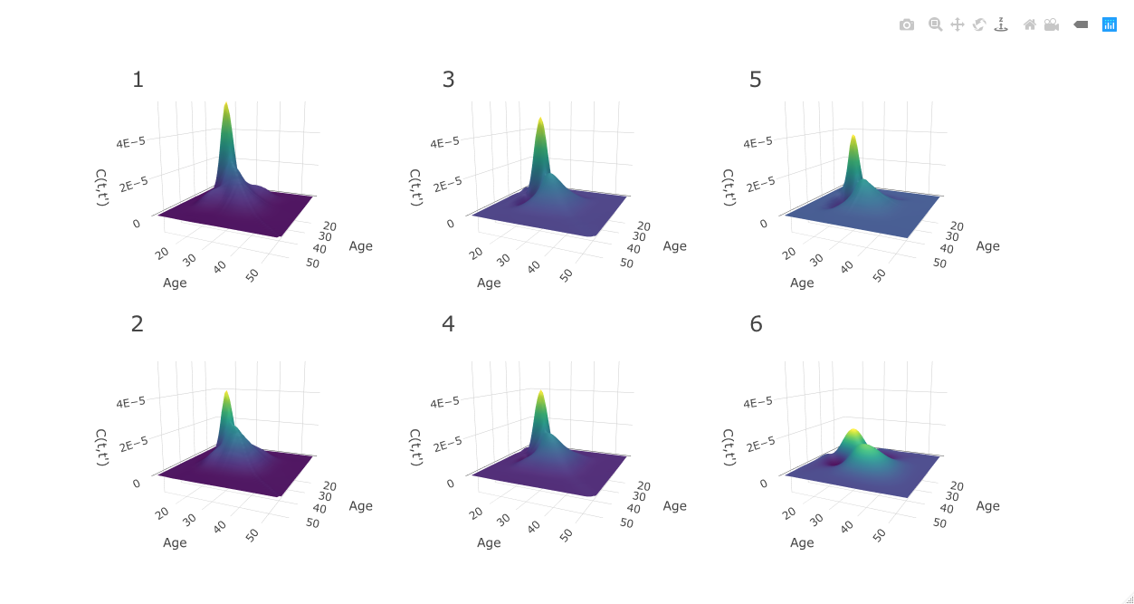
Next we conduct an eigen-analysis of the covariance structure for both cohorts separately. Figure 5 plots eigenfunctions of the marginal covariances over ERP time and trials. Credible intervals are calculated following Crainiceanu and others 2007.
We start by analyzing summaries indexing variability in ERP time. For both the TD and ASD cohorts, the first eigenfunction explains the vast majority of the marginal covariance (84%-88% in ASD, and 86%-90% in TD). In both groups this first eigenfunction is relatively flat and can be interpreted as representing variability in the overall level of condition differentiation within a trial. The magnitude and shape of variation is comparable between TD and ASD children. Finer differences may be detected in the second and third eigenfunction, which further characterize variability in the shape of the ERP waveforms about the P300 peak. For both cohorts, however, these summaries represent only a small percentage of the variance in ERP waveform within trial.
Perhaps more interesting is an analysis of the marginal covariance across trial, as probabilistic learning patterns are likely to unfold with prolonged exposure to expected vs. unexpected shape pairings. For the ASD group, the first eigenfunction dips in an approximately quadratic fashion, suggesting enhanced variability in condition differentiation at around trial 35. Similarly, for the TD group, the first trial eigenfunction has a slight peak around trial 25. A possible interpretation of these covariance components relates to implicit learning, with higher variance in differentiation occurring earlier for TD than for ASD children. For both TD and ASD, the second eigenfunction across trials is can be interpreted as a contrast between high condition differentiation at early trials and low condition differentiation at later trials. Finally for the ASD cohort, the third eigenfunction exhibits a peak around trial 30. A possible interpretation would identify heterogeneity in the timing of learning, with some of the trajectories inducing variation in condition differentiation around trial 30, as opposed to the first eigenfunction identifying increased variance at around trial 35. Similarly for the TD group, the third trial eigenfunction has a dip around trial 35, indexing delayed increased variability in condition differentiation around trial 35.
7 Discussion
In this paper we provide a probabilistic characterization of longitudinal-functional data. As part of our work we propose a joint framework for the estimation of the mean or the regression function, and a flexible prior for covariance operators. Regularized estimation relies crucially on the projection of a set of basis coefficients onto a latent subspace, with adaptive shrinkage achieved via a broadly supported class of product Gamma priors. While we have not established theoretical results on posterior consistency, we have shown that the proposed framework exhibits competitive operating characteristics, when compared with alternative modeling strategies.
Importantly, uncertainty quantification, is achieved without having to rely on the asymptotic performance of bootstrap methods. From an applied perspective, analysts are charged with choosing the appropriate projection space. However, we see this as a feature rather than a problem, as different data scenarios may require and motivate the used of alternative basis systems. Because regularization is achieved jointly with estimation, inference is straightforward and does not need to account separately for the estimation of nuisance parameters or the choice of a finite number of eigenfunction to use in a truncated version of the model, as is the case for FPCA-based methods.
We have shown that posterior inference using MCMC is implemented in a relatively straightforward fashion and need not rely on complicated posterior sampling strategies. When dealing with large data-sets, this naïve inferential strategy may not be appropriate. For example, the computation of marginal covariance functions and can be slow for designs with many longitudinal or functional time points, as numerical marginalization requires the computation of a four dimensional covariance function . Some potential solutions include considering approximate computation through variational Bayes, or MAP approximation based on EM strategies.
From a modeling perspective, our probabilistic characterization of the longitudinal-functional covariance function is essentially equivalent to the weakly-separable model of Chen and others 2017. While more general than a strictly separable model, this strategy makes strong assumptions about the structure of a high-dimensional covariance operator. Testing strategies have been developed in the literature (Lynch and Chen 2017). However, we find that a more natural approach to the problem is one of regularized estimation. In this setting, a possible extension of our modeling framework could include an embedding strategy for the regularization of a non-separable covariance operator towards a weakly separable one.
8 Software
Software in the form of an R package including complete documentation and a sample data set is available from https://github.com/jshamsho/LFBayes
9 Supplementary Material
Supplementary material is available online at http://biostatistics.oxfordjournals.org.
Acknowledgments
Conflict of Interest: None declared.
References
- Bhattacharya and Dunson (2011) Bhattacharya, A. and Dunson, D.B. (2011). Sparse bayesian infinite factor models. Biometrika 98, 291–306.
- Chen and others (2017) Chen, K., Delicado, P. and Müller, H.G. (2017). Modelling function-valued stochastic processes, with applications to fertility dynamics. Journal of the Royal Statistical Society, Series B 79(1), 177–196.
- Chen and Müller (2012) Chen, K. and Müller, H.G. (2012). Modeling repeated functional observations. Journal of the American Statistical Association 107(500), 1599–1609.
- Crainiceanu and others (2007) Crainiceanu, C.M., Ruppert, D., Carroll, R.J., Joshi, A. and Goodner, B. (2007). Spatially adaptive bayesian penalized splines with heteroscedastic errors. Journal of Computational and Graphical Statistics 16, 265–288.
- Cuevas and others (2006) Cuevas, A., Febrero, M. and Fraiman, R. (2006). On the use of the bootstrap for estimating functions with functional data. Computational Statistics & Data Analysis 51(2), 1063 – 1074.
- Delattre and others (2014) Delattre, M., Lavielle, M. and Poursat, M. (2014). A note on bic in mixed-effects models. Electron. J. Statist. 8(1), 456–475.
- Di and others (2009) Di, C-Z., Crainiceanu, C. M., Caffo, B. S. and Punjabi, N. M. (2009, 03). Multilevel functional principal component analysis. Ann. Appl. Stat. 3(1), 458–488.
- Ferraty and others (2010) Ferraty, F., Van Keilegom, I. and Vieu, P. (2010). On the validity of the bootstrap in non-parametric functional regression. Scandinavian Journal of Statistics 37(2), 286–306.
- Gneiting (2002) Gneiting, T. (2002). Nonseparable, stationary covariance functions for space-time data. Journal of the American Statistical Association 97(458), 590–600.
- Goldsmith and others (2016) Goldsmith, J., Liu, X., Jacobson, J.S. and Rundle, A. (2016, 09). New insights into activity patterns in children, found using functional data analyses. Medicine and science in sports and exercise 48(9), 1723–1729.
- Greven and others (2010) Greven, S., Crainiceanu, C., Caffo, B. and Reich, D. (2010). Longitudinal functional principal component analysis. Electron. J. Statist. 4, 1022–1054.
- Hasenstab and others (2017) Hasenstab, K., Scheffler, A., Telesca, D., Sugar, C. A., Jeste, S., DiStefano, C. and Şentürk, D. (2017). A multi-dimensional functional principal components analysis of eeg data. Biometrics 73(3), 999–1009.
- Hasenstab and others (2015) Hasenstab, K., Sugar, C. A., Telesca, D., McEvoy, K., Jeste, S. and Şentürk, D. (2015). Identifying longitudinal trends within eeg experiments. Biometrics 71(4), 1090–1100.
- HFD (2019) HFD. (2019). Human fertility database. Max Planck Institute for Demographic Research (Germany) and Vienna Institute of Demography (Austria).
- Jeste and others (2015) Jeste, S. S., Kirkham, N., Senturk, D., Hasenstab, K., Sugar, C., Kupelian, C., Baker, E., Sanders, A. J., Shimizu, C., Norona, A., Paparella, T., Freeman, S. F.N. and others. (2015). Electrophysiological evidence of heterogeneity in visual statistical learning in young children with asd. Developmental Science 18(1), 90–105.
- Lee and others (2019) Lee, W., Miranda, M. F., Rausch, P., Baladandayuthapani, V., Fazio, M., Downs, J. C. and Morris, J. S. (2019, 04). Bayesian semiparametric functional mixed models for serially correlated functional data, with application to glaucoma data. Journal of the American Statistical Association 114(526), 495–513.
- Lord and others (2000) Lord, C., Risi, S., Lambrecht, L., Cook, E. H., Leventhal, B. L., DiLavore, P. C., Pickles, A. and Rutter, M. (2000). The autism diagnostic observation schedule— generic: A standard measure of social and communication deficits associated with the spectrum of autism. ournal of autism and developmental disorders 30(3), 205–223.
- Lynch and Chen (2017) Lynch, B. and Chen, K. (2017, March). A test of weak separability for multi-way functional data, with application to brain connectivity studies. arXiv e-prints, arXiv:1703.10210.
- Montagna and others (2012) Montagna, S., Tokdar, S., Neelon, B. and Dunson, D.B. (2012). Bayesian latent factor regression for functional and longitudinal data. Biometrics 68, 1064–1073.
- Morris and others (2003) Morris, J. S., Vannucci, M., Brown, P. J. and Carroll, R. J. (2003). Wavelet-based nonparametric modeling of hierarchical functions in colon carcinogenesis. Journal of the American Statistical Association 98(463), 573–583.
- Park and Staicu (2015) Park, S.Y. and Staicu, A. (2015). Longitudinal functional data analysis. Stat 4(1), 212–226.
- Ren and others (2010) Ren, S., Lai, H., Tong, W., Aminzadeh, M., Hou, X. and Lai, S. (2010). Nonparametric bootstrapping for hierarchical data. Journal of Applied Statistics 37(9), 1487–1498.
- Scheffler and others (2018) Scheffler, A., Telesca, D., Li, Q., Sugar, C., Distefano, C., Jeste, S. and Şentürk, D. (2018, 08). Hybrid principal components analysis for region-referenced longitudinal functional EEG data. Biostatistics.
- Shi and Choi (2011) Shi, J.Q. and Choi, T. (2011). Gaussian Process Regression Analysis for Functional Data. New York: Chapman and Hall/CRC.
- Suarez and Ghosal (2017) Suarez, A.J. and Ghosal, S. (2017, 06). Bayesian estimation of principal components for functional data. Bayesian Anal. 12(2), 311–333.
- Yang and others (2017) Yang, J., Cox, D.D., Lee, J.S. and Choi, P. Ren T. (2017). Efficient bayesian hierarchical functional data analysis with basis function approximations using gaussian-wishart processes. Biometrics 73(4), 1082–1091.
- Yang and others (2016) Yang, J., Zhu, H., Choi, T. and Cox, D.D. (2016, 09). Smoothing and mean–covariance estimation of functional data with a bayesian hierarchical model. Bayesian Anal. 11(3), 649–670.
| Case 1 | Bayes | Product | Empirical | |
|---|---|---|---|---|
| .014 (.005, .038) | .019 (.010, .044) | .019 (.010, .044) | ||
| .062 (.023, .224) | .085 (.047, .200) | .151 (.097, .297) | ||
| .007 (.003, .019) | .010 (.005, .021) | .010 (.005, .021) | ||
| .030 (.010, .097) | .057 (.038, .128) | .076 (.050, .151) | ||
| Case 2 | ||||
| .024 (.007, .101) | .031 (.013, .118) | .031 (.013, .118) | ||
| .039 (.011, .184) | .050 (.012, .202) | .067 (.030, .228) | ||
| .014 (.004, .054) | .017 (.007, .062) | .017 (.007, .062) | ||
| .019 (.005, .091) | .024 (.007, .093) | .032 (.014, .106) | ||
| Case 3 | ||||
| .155 (.046, .389) | .160 (.051, .393) | .160 (.051, .393) | ||
| .051 (.016, .187) | .051 (.014, .183) | .067 (.023, .200) | ||
| .073 (.019, .216) | .076 (.021, .219) | .076 (.021, .219) | ||
| .028 (.008, .091) | .027 (.007, .089) | .034 (.011, .099) | ||
| (, ) | DIC | BIC 1 | BIC 2 |
|---|---|---|---|
| (5, 5) | 1.29 (1.20, 1.37) | 1.49 (1.40, 1.57) | 1.59 (1.51, 1.67) |
| (10, 10) | 1.22 (1.14, 1.29) | 1.40 (1.32, 1.47) | 1.50 (1.43, 1.57) |
| (15, 15) | 1.24 (1.16, 1.31) | 1.41 (1.33, 1.48) | 1.52 (1.43, 1.59) |



| ASD |
 |
| TD |
 |