Fixed Point Analysis of Douglas-Rachford Splitting for Ptychography and Phase RetrievalThanks: ^∗Corresponding author: fannjiang@math.ucdavis.eduThanks: SIAM Journal on Imaging Sciences (2020)

Albert Fannjiang^∗ and Zheqing Zhang Address: Department of Mathematics, University of California, Davis, California 95616, USA. Address: Department of Mathematics, University of California, Davis, California 95616, USA.

Abstract.

Douglas-Rachford Splitting (DRS) methods based on the proximal point algorithms for the Poisson and Gaussian log-likelihood functions are proposed for ptychography and phase retrieval.

Fixed point analysis shows that the DRS iterated sequences are always bounded explicitly in terms of the step size and that the fixed points are attracting if and only if the fixed points are regular solutions. This alleviates two major drawbacks of the classical Douglas-Rachford algorithm: slow convergence when the feasibility problem is consistent and divergent behavior when the feasibility problem is inconsistent.

Fixed point analysis also leads to a simple, explicit expression for the optimal step size in terms of the spectral gap of an underlying matrix.

When applied to the challenging problem of blind ptychography, which seeks to recover both the object and the probe simultaneously, Alternating Minimization with the DRS inner loops, even with a far from optimal step size, converges geometrically under the nearly minimum conditions established in the uniqueness theory.

1. Introduction

Phase retrieval may be posed as an inverse problem in which an object vector with certain properties is to be reconstructed from the intensities of its Fourier transform. By encoding the properties and the Fourier intensities as constraint sets, phase retrieval can be cast as a feasibility problem, i.e. the problem of finding a point in the intersection of the constraint sets. The challenge is that the intensities of the Fourier transform results in a non-convex constraint set (a high dimensional torus of variable radii).

Projection algorithms comprise a general class of iterative methods for solving feasibility problems by projecting onto each of the constraint sets at each step [1]. The most basic projection algorithm is von Neumann’s Alternating Projections (AP) (aka Error Reduction in phase retrieval [23]). However, AP tends to stagnate when applied to phase retrieval, resulting in poor performance.

A better method than AP is the classical Douglas-Rachford algorithm (a.k.a. Averaged Alternating Reflections (AAR)) [13, 25, 35, 25], which apparently can avoid the stagnation problem in many non-convex problems. When applied to phase retrieval, the classical Douglas-Rachford algorithm is a special case of Fienup’s Hybrid-Input-Output algorithm [3, 23].

In addition to the standard phase retrieval, AAR has been applied to ptychography under the name of difference map [51, 50, 54]. Ptychography uses a localized coherent probe to illuminate different parts of a unknown extended object and collect multiple diffraction patterns as measurement data (Figure 1). The redundant information in the overlap between adjacent illuminated spots is then exploited to improve phase retrieval methods [47, 44]. Recently ptychography has been extended to the Fourier domain [57, 45]. In Fourier ptychography, illumination angles are scanned sequentially with a programmable array source with the diffraction pattern measured at each angle [53, 32]. Tilted illumination samples different regions of Fourier space, as in synthetic-aperture and structured-illumination imaging.

Local, linear convergence of AAR as applied to phase retrieval as well as ptychography was recently proved in [9, 10]. Conditions for global convergence, however, are not known. Numerical evidence points to sub-linear rate when convergence happens. On the other hand, for inconsistent feasibility problems, AAR iteration is known to diverge to infinity even in the convex case (see Proposition 2.1(ii)). This poses a great challenge to AAR when the data contain noise because in phase retrieval the dimension of the measurement data is much higher than that of the unknown object (an over-determined system).

The purpose of this work is to develop reconstruction schemes based on more general Douglas-Rachford splitting (DRS) with adjustable step sizes, perform the fixed point analysis and demonstrate numerical convergence. AAR is the limiting case of DRS.

The DRS method is an optimization method based on proximal operators, a natural extension of projections, and is closely related to the Alternating Direction Method of Multipliers (ADMM). The performance of DRS and ADMM in the non-convex setting depends sensitively on the choice of the loss functions as well as the step sizes. Typically, global convergence of DRS requires a loss function possessing a uniformly Lipschitz gradient and sufficiently large step sizes [9, 33, 30], both of which, however, tend to hinder the performance of DRS.

In this paper, the loss functions are based on the log-likelihood function for the most important Poisson noise, which does not have a uniformly Lipschitz gradient, with an optimal step size, which is necessarily quite large.

We show by a fixed point analysis that the DRS method is well behaved in the sense that the DRS iterated sequences are always bounded (explicitly in terms of the step size) and that the fixed points are attracting if and only if the fixed points are regular solutions. In other words, the DRS methods remove AAR’s two major drawbacks: slow convergence when the feasibility problem is consistent and divergent behavior when the feasibility problem is inconsistent.

Moreover, the fixed point analysis leads to the determination of the optimal step size and, along with it, simple and efficient algorithms with no tuning parameter (Averaged Projection-Reflection). The main application considered is the more challenging form of ptychography called blind ptychography which seeks to recover both the unknown object and the probe function simultaneously. When properly initialized, the DRS algorithms with the optimal step size converge globally and geometrically to the true solution modulo the inherent ambiguities.

Refer to caption — Figure 1. Simplified ptychographic setup showing a Cartesian grid used for the overlapping raster scan positions [43]. See Appendix A for details.

The rest of the paper is organized as follows. In Section 3, we introduce the Douglas-Rachford splitting method as the key ingredient of our reconstruction algorithms, Gaussian-DRS and Poisson-DRS. We give the fixed point and stability analysis in Sections 4, 5 and 6. In Section 7, we discuss the selection of the optimal step size. In Section 8, we discuss the application to blind ptychography and in Section 9, we present numerical experiments. In Appendix A, we discuss the structure of the measurement matrices. In Appendix B, we show that Gaussian-DRS is an asymptotic form of Poisson-DRS. In Appendix D we give a perturbation analysis for the Poisson DRS. In Appendix E, we analyze the eigenstructure of the measurement matrices. We conclude in Section 10. A preliminary version of the present work is given in [20].

2. Averaged Alternating Reflections (AAR)

The classical Douglas-Rachford algorithm is based on the following characterization of convex feasibility problems.

Let $X$ and $Y$ be the constraint sets. Let $P_{X}$ be the projection onto $X$ and $R_{X}=2P_{X}-I$ the corresponding reflector. $P_{Y}$ and $R_{Y}$ are defined likewise. Then

(1)

\displaystyle u\in X\cap Y\quad\mbox{if and only if }\quad u=R_{Y}R_{X}u

[26]. The latter fixed point equation motivates the Peaceman-Rachford (PR) method: For $k=0,1,2,\ldots$

u_{k+1}=R_{Y}R_{X}y_{k}.

The classical Douglas-Rachford algorithm is the averaged version of PR: For $k=0,1,2,\ldots$

(2)

\displaystyle u_{k+1}={1\over 2}u_{k}+{1\over 2}R_{Y}R_{X}u_{k},

hence the name Averaged Alternating Reflections (AAR).

A standard result for AAR in the convex case is this.

Proposition 2.1.

[5] Suppose $X$ and $Y$ are closed and convex sets of a finite-dimensional vector space $E$ . Let $\{u_{k}\}$ be an AAR-iterated sequence for any $u_{1}\in E$ . Then one of the following alternatives holds:

(i) $X\cap Y\neq\emptyset$ and $(u_{k})$ converges to a point $u$ such that $P_{X}u\in X\cap Y$ ;
(ii) $X\cap Y=\emptyset$ and $\|u_{k}\|\to\infty$ .

In the consistent case (i), the limit point $u$ is a fixed point of the AAR map (2), which after projection is in $X\cap Y$ . However, the convergence rate of AAR is in general sublinear [29, 2]. The inconsistent case (ii) arises from noisy data or modeling errors resulting in divergent AAR iterated sequences, a major drawback of AAR since the inconsistent case is prevalent with noisy data because of the higher dimension of data compared to the object.

The AAR map (2) is often written in the following form

(3)

\displaystyle u_{k+1}=u_{k}+P_{Y}R_{X}u_{k}-P_{X}u_{k}

which is equivalent to the 3-step iteration

(4)	$\displaystyle y_{k}$	$\displaystyle=$	$\displaystyle P_{X}u_{k};$
(5)	$\displaystyle z_{k}$	$\displaystyle=$	$\displaystyle P_{Y}(2y_{k}-u_{k})=P_{Y}R_{X}u_{k}$
(6)	$\displaystyle u_{k+1}$	$\displaystyle=$	$\displaystyle u_{k}+z_{k}-y_{k}$

2.1. Phase retrieval as feasibility

For any finite dimensional vector $u$ , define its modulus vector $|u|$ as $|u|[j]=|u[j]|$ and its phase vector $\mbox{\rm sgn}(u)$ as

\mbox{\rm sgn}(u)[j]=\left\{\begin{matrix}1&\mbox{if $u[j]=0$}\\ u[j]/|u[j]|&\mbox{else. }\end{matrix}\right.

where $j$ is the index for the vector component. Because of the value of $\mbox{\rm sgn}(u)$ where $u[j]=0$ is arbitrarily selected, such points are points of discontinuity of the sgn function.

In phase retrieval including ptychography, we can write the given data $b$ as

(7)

\displaystyle b=|u|\quad\mbox{ with}\quad u=Af

for some measurement matrix $A$ and unknown object $f$ . For phase retrieval and ptychography, $A$ has some special features described in Appendix A. For most of the subsequent analysis, however, these special features are not relevant.

Let $O$ be the object space, typically a finite-dimensional complex vector space, and $X=AO$ . Since the object is a two dimensional, complex-valued image, we let $O=\mathbb{C}^{n^{2}}$ where $n$ is the number of pixels in each dimension.

Let $N$ be the total number of data. The data manifold

Y:=\{u\in\mathbb{C}^{N}:|u|=b\}

is a $N$ (real) dimensional torus. For phase retrieval it is necessary that $N>2n^{2}$ . Without loss of generality we assume that $A$ has a full rank.

The problem of phase retrieval and ptychography can be formulated as the feasibility problem

(8)

\displaystyle\hbox{Find}\quad u\in X\cap Y,

in the transform domain $\mathbb{C}^{N}$ instead of the object domain $\mathbb{C}^{n^{2}}$ .

Let us clarify the meaning of solution in the transform domain since $A$ is overdetermining. Let $\odot$ denotes the component-wise (Hadamard) product and we can write

(9)		$\displaystyle P_{X}u=AA^{+}u,$		$\displaystyle P_{Y}u=b\odot\mbox{\rm sgn}(u)$
	$\displaystyle R_{X}=2P_{X}-I,$		$\displaystyle R_{Y}=2P_{Y}-I$

where $A^{+}:=(A^{*}A)^{-1}A^{*}$ is the pseudo-inverse of $A$ .

We refer to $u=e^{{\rm i}\alpha}Af,\alpha\in\mathbb{R}$ , as the true solution (in the transform domain), up to a constant phase factor $e^{{\rm i}\alpha}$ . We say that $u$ is a generalized solution (in the transform domain) if

|\hat{u}|=b,\quad\hat{u}:=P_{X}u.

Accordingly, the alternative (i) in Proposition 2.1 means that if a convex feasibility problem is consistent then every AAR iterated sequence converges to a generalized solution and hence every fixed point is a generalized solution.

Typically a generalized solution $u$ is neither a feasible solution (since $|u|$ may not equal $b$ ) nor unique (since $A$ is overdetermining) and, if $P_{X}z=0$ , $u+z$ is also a generalized solution. We call $u$ a regular solution if $u$ is a generalized solution and $P_{X}u=u$ .

Let $\hat{u}=P_{X}u$ for a generalized solution $u$ . Since $P_{X}\hat{u}=\hat{u}$ and $|\hat{u}|=b$ , $\hat{u}$ is a regular solution. Let us state this simple fact for easy reference.

Proposition 2.2.

If $u$ is a generalized solution, then $P_{X}u$ is a regular solution.

The goal of the inverse problem (7) is the unique determination of $f$ , up to a constant phase factor, from the given data $b$ . In other words, uniqueness holds if, and only if, all regular solutions $\hat{u}$ have the form

(10)

\displaystyle\hat{u}=e^{{\rm i}\alpha}Af

or equivalently, any generalized solution $u$ is an element of the $(2N-2n^{2})$ -dimensional manifold

(11)

\displaystyle\{e^{{\rm i}\alpha}Af-z:P_{X}z=0,\,\,z\in\mathbb{C}^{N},\,\,\alpha\in\mathbb{R}\}.

In the transform domain, the uniqueness is characterized by the uniqueness of the regular solution, up to a constant phase factor. Geometrically, uniqueness means that the intersection $X\cap Y$ is a circle (parametrized $e^{{\rm i}\alpha}$ times $Af$ ).

As proved in [9], when the uniqueness (11) holds, the fixed point set of the AAR map (2) is exactly the continuum set

(12)

\displaystyle\{u=e^{{\rm i}\alpha}Af-z:P_{X}z=0,\,\,\mbox{\rm sgn}(u)=\alpha+\mbox{\rm sgn}(Af),\,\,z\in\mathbb{C}^{N},\alpha\in\mathbb{R}\}.

In (12), the phase relation $\mbox{\rm sgn}(u)=\alpha+\mbox{\rm sgn}(Af)$ implies that $z=\eta\odot\mbox{\rm sgn}(u),\eta\in\mathbb{R}^{N},b+\eta\geq 0.$ So the set (12) can be written as

(13)

\displaystyle\{e^{{\rm i}\alpha}(b-\eta)\odot\mbox{\rm sgn}(Af):P_{X}(\eta\odot\mbox{\rm sgn}(Af))=0,\,\,b+\eta\geq 0,\,\,\eta\in\mathbb{R}^{N},\alpha\in\mathbb{R}\},

which is an $(N-2n^{2})$ real-dimensional set, a much larger set than the circle $\{e^{{\rm i}\alpha}Af:\alpha\in\mathbb{R}\}$ for a given $f$ . On the other hand, the fixed point set (13) is $N$ -dimension lower than the set (11) of generalized solutions.

A more intuitive characterization of the fixed points can be obtained by applying $R_{X}$ to the set (13). Since

R_{X}[e^{{\rm i}\alpha}(b-\eta)\odot\mbox{\rm sgn}(Af)]=e^{{\rm i}\alpha}(b+\eta)\odot\mbox{\rm sgn}(Af)

amounting to the sign change in front of $\eta$ , the image set of (13) under the map $R_{X}$ is

(14)

\displaystyle\{e^{{\rm i}\alpha}(b+\eta)\odot\mbox{\rm sgn}(Af):P_{X}(\eta\odot\mbox{\rm sgn}(Af))=0,\,\,b+\eta\geq 0,\,\,\eta\in\mathbb{R}^{N},\alpha\in\mathbb{R}\}.

The set (14) is the fixed point set of the alternative form of AAR:

(15)

\displaystyle x_{k+1}

\displaystyle=

\displaystyle{1\over 2}x_{k}+{1\over 2}R_{X}R_{Y}x_{k}

in terms of $x_{k}:=R_{X}u_{k}$ . The expression (14) says that the fixed points of (15) are generalized solutions with the “correct” Fourier phase.

However, the boundary points of the fixed point set (14) are degenerate in the sense that they have vanishing components, i.e. $(b+\eta)[j]=0$ for some $j$ and can slow down convergence [24]. Such points are points of discontinuity of the AAR map (15) because they are points of discontinuity of $P_{Y}=b\odot\mbox{\rm sgn}(\cdot)$ (see also the comment below (30)). Indeed, even though AAR converges linearly in the vicinity of the true solution, numerical evidence suggests that globally (starting with a random initial guess) AAR converges sub-linearly (cf. [29, 2]). Due to the non-uniformity of convergence, the additional step of applying $P_{X}$ (Proposition 2.1(i)) at the “right timing” of the iterated process can jumpstart the geometric convergence regime [9].

3. Douglas-Rachford Splitting (DRS)

Douglas-Rachford Splitting (DRS) is an optimization method for solving the following minimization problem:

(16)

\min\limits_{u}K(u)+L(u)

where the loss functions $L$ and $K$ represent the data constraint $Y$ and the object constraint $X$ , respectively.

To deal with the divergence behavior of AAR (Proposition 2.1 (ii)) in the case of, e.g. noisy data, we consider the Poisson log-likelihood cost functions [52, 6]

(17)

\displaystyle\mbox{\rm Poisson:}\quad L(u)

\displaystyle=

\displaystyle\sum_{i}|u[i]|^{2}-b^{2}[i]\ln|u[i]|^{2}

based on the maximum likelihood principle for the Poisson noise model. The Poisson noise is the most prevalent noise in X-ray coherent diffraction. There is, however, a disadvantage of working with (17), i.e. it has a divergent derivative where $u(i)$ vanishes but $b(i)$ does not. This roughness can be softened by considering an asymptotic form

(18)

\displaystyle\mbox{\rm Gaussian:}\quad L(u)

\displaystyle=

\displaystyle{1\over 2}\||u|-b\|^{2}

In Appendix B, we show that the Poisson log-likelihood function (17) is asymptotically reducible to (18).

With the constraint $u=Ag$ , $g$ is a stationary point in the object domain if and only if

\displaystyle g

\displaystyle=

\displaystyle A^{*}\left[\mbox{\rm sgn}(Ag)\odot b\right].

In the noiseless case, $|Af|=b$ and hence $f$ is a stationary point by the isometry of $A$ . On the other hand, with noisy data there is no regular solution to $|Ax|=b$ with high probability (since $A$ has many more rows than columns) and $f$ is unlikely to be a stationary point (since the stationarity equation imposes extra constraints on noise).

Moreover, the Hessian of (18) at $u=Af$ is positive semi-definite and has one-dimensional eigenspace spanned by ${\rm i}f$ associated with eigenvalue zero [9, 10, 11].

Expanding the loss function (18)

(19)

\displaystyle L(u)

\displaystyle=

\displaystyle\frac{1}{2}\|u\|^{2}-\sum_{j}b[j]|u[j]|+\frac{1}{2}\|b\|^{2}

we see that $L$ has a bounded sub-differential where $u[j]$ vanishes but $b[j]$ does not. There are various tricks to further smooth out (18) e.g. by introducing an additional regularization parameter as

(20)

\displaystyle L(u)

\displaystyle=

\displaystyle{1\over 2}\|\sqrt{|u|^{2}+\epsilon}-\sqrt{b^{2}+\epsilon}\|^{2},\quad\epsilon>0

(see e.g. [8]).

Besides the Poisson noise, a type of noise due to interference from multiple scattering can be modeled as complex circularly-symmetric Gaussian noise, resulting in the signal model

(21)

\displaystyle b

\displaystyle=

\displaystyle|Af+\eta|

where $\eta$ is a complex circularly-symmetric Gaussian noise. Squaring the expression, we obtain

\displaystyle b^{2}

\displaystyle=

\displaystyle|Af|^{2}+|\eta|^{2}+2\Re(\overline{\eta}\odot Af)

Suppose $|\eta|\ll|Af|$ so that $|\eta|^{2}\ll 2\Re(\overline{\eta}\odot Af)$ . Then

(22)

\displaystyle b^{2}

\displaystyle\approx

\displaystyle|Af|^{2}+2\Re(\overline{\eta}\odot Af).

Eq. (22) says that at the photon counting level, the noise appears additive and Gaussian but with variance proportional to $|Af|^{2}$ , the Poisson noise in the asymptotic regime discussed in Appendix B. Therefore the loss function (18) is suitable for this case too.

The maximum likelihood scheme is a variance stabilization scheme which uniformizes the probability distribution for every pixel regardless of the measured intensity value [31]. See [28, 56] for more choices of loss functions.

The amplitude-based Gaussian loss function (18) is well known to outperforms the intensity-based loss function ${1\over 2}\||u|^{2}-b^{2}\|^{2}$ , even though the latter is more smooth [55]. Due to the non-differentiability of both $K$ and $L$ , the global convergence property of the proposed DRS optimization is beyond the current framework of analysis [33]. The ptychographic iterative engines, PIE [21, 22, 48], ePIE [40] and rPIE [38], are also related to the mini-batch gradient method for the amplitude-based cost function (18).

For $K$ , we let $K(u)$ be the indicator function of the range of $A$ , i.e. a “hard” constraint.

When the corresponding feasibility problem is consistent (feasible), there exist $u\in\mathbb{C}^{N}$ such that $|u|=b$ and $u=Ag$ for some $g\in\mathbb{C}^{n^{2}}$ , which are exactly the global minimizers of (16), realizing the minimum value 0, as well as the regular solutions defined in Section 2.1.

When the corresponding feasibility problem is inconsistent (infeasible), the minimum value of (16) is unknown and the global minimizers are harder to characterize.

DRS is based on the proximal operator which is a generalization of projection. The proximal point relative to a function $G$ is given by

\hbox{prox}_{G}(u):=\mathop{\text{argmin}}\limits_{x}G(x)+\frac{1}{2}\|x-u\|^{2}.

With the loss functions (17) or (18), $P_{X}$ is replaced by $P_{K/\rho}$ and $P_{Y}$ by $P_{L/\rho}$ , respectively, with the step size $\gamma=1/\rho$ . The 3-step procedure (4)-(6) is replaced by

(23)	$\displaystyle v_{l}$	$\displaystyle=$	$\displaystyle\hbox{prox}_{K/\rho}(u_{l});$
(24)	$\displaystyle w_{l}$	$\displaystyle=$	$\displaystyle\hbox{prox}_{L/\rho}(2v_{l}-u_{l})$
(25)	$\displaystyle u_{l+1}$	$\displaystyle=$	$\displaystyle u_{l}+w_{l}-v_{l}$

for $l=1,2,3\ldots$ .

For convex optimization, DRS (23)-(25) is equivalent to the Alternating Direction Method of Multipliers (ADMM) applied to the dual problem to (16). In Appendix C, we show that for phase retrieval they are essentially equivalent to each other.

For our choice of $K$ , $\hbox{prox}_{K/\rho}(u)=P_{X}u=AA^{+}u$ is independent of $\rho$ . This should be contrasted with the choice of the more smooth distance function adopted in [33] for the tractability of convergence analysis (see more discussion in Section 10).

If we define the reflector ${\mathcal{R}}_{Y}$ corresponding to $\hbox{prox}_{L/\rho}(u)$ as

(26)

\displaystyle{\mathcal{R}}_{Y}u:=2\,\,\hbox{prox}_{L/\rho}(u)-u,

then we can write the system (23)-(25) as

(27)

\displaystyle u_{k+1}={1\over 2}u_{k}+{1\over 2}{\mathcal{R}}_{Y}R_{X}u_{k}

which is equivalent to

(28)

\displaystyle x_{k+1}={1\over 2}x_{k}+{1\over 2}R_{X}{\mathcal{R}}_{Y}x_{k}

in terms of $x_{k}:=R_{X}u_{k}$ . In other words, the order of carrying out $\hbox{prox}_{L/\rho}$ and $\hbox{prox}_{K/\rho}$ does not matter in the current DRS set-up.

For the Gaussian loss function (18), the proximal point can be explicitly derived

	$\displaystyle\hbox{prox}_{L/\rho}(u)$	$\displaystyle=$	$\displaystyle\frac{1}{\rho+1}b\odot\mbox{\rm sgn}{(u)}+\frac{\rho}{\rho+1}u$
		$\displaystyle=$	$\displaystyle\frac{1}{\rho+1}(b+\rho\|u\|)\odot\mbox{\rm sgn}{(u)},$

an averaged projection with the relaxation parameter $\rho$ . Now we are ready to give the most compact and explicit representation of the Gaussian DRS map:

(29)		$\displaystyle u_{k+1}$	$\displaystyle=$	$\displaystyle\frac{u_{k}}{\rho+1}+\frac{\rho-1}{\rho+1}P_{X}u_{k}+\frac{1}{\rho+1}P_{Y}R_{X}u_{k}$
(29)			$\displaystyle:=$	$\displaystyle\Gamma(u_{k})$

which can be compared with AAR in the form (3).

For the Poisson case the DRS map has a more complicated form

(30)		$\displaystyle u_{k+1}$	$\displaystyle=$	$\displaystyle{1\over 2}u_{k}-{1\over\rho+2}R_{X}u_{k}+\frac{\rho}{2(\rho+2)}\left[\|R_{X}u_{k}\|^{2}+\frac{8(2+\rho)}{\rho^{2}}b^{2}\right]^{1/2}\odot\mbox{\rm sgn}{\Big(R_{X}u_{k}\Big)}$
(30)			$\displaystyle:=$	$\displaystyle\Pi(u_{k})$

where $b^{2}$ is the vector with component $b^{2}[j]=(b[j])^{2}$ for all $j$ .

Note that $\Gamma(u)$ and $\Pi(u)$ are continuous except where $R_{X}u$ vanishes but $b$ does not due to arbitrariness of the value of the sgn function at zero.

After the iteration is terminated with the terminal vector $u_{*}$ , the object estimate is obtained by

(31)

\displaystyle f_{*}=A^{+}u_{*}.

We shall refer to DRS with the Poisson log-likelihood function (30) and the Gaussian version (29) by Poisson-DRS and Gaussian-DRS, respectively. The computation involved in Gaussian-DRS and Poisson-DRS are mostly pixel-wise operations (hence efficient) except for the pseudo-inverse $A^{+}$ which can be computed efficiently (see Appendix A).

In the limiting case of $\rho=0$ , both Gaussian-DRS and Poisson-DRS become the AAR algorithm.

4. Fixed points

For simplicity of presentation, we shall focus on the case of the Gaussian DRS.

By definition, all fixed points $u$ satisfy the equation

(32)

\displaystyle u

\displaystyle=

\displaystyle\Gamma(u)

and hence after some algebra by (29)

(33)

\displaystyle P_{X}u+\rho P^{\perp}_{X}u=b\odot\mbox{\rm sgn}(R_{X}u).

The main result of this section is that the iteration of $\Gamma$ always produces a sequence bounded in norm by

{\|b\|\over\min\{\rho,1\}}\quad\mbox{\quad for \quad}\quad\rho>0

(Theorem 4.6) with slightly better bounds on the fixed points (Corollary 4.7). Therefore, Gaussian-DRS is free of the divergence problem associated with AAR in the infeasible case.

It is often convenient to perform the analysis in terms of the pair of variables $u$ and $x:=R_{X}u$ . Here are some basic relations between $u$ and $x$ .

Proposition 4.1.

For any $u\in\mathbb{C}^{N}$ , $x:=R_{X}u$ satisfies

\displaystyle u=R_{X}x,

\displaystyle P_{X}u=P_{X}x,

\displaystyle P^{\perp}_{X}u=-P^{\perp}_{X}x.

Proof.

First note that

R_{X}x=2P_{X}x-x=2P_{X}u-(2P_{X}u-u)=u.

Moreover,

\displaystyle P_{X}x=P_{X}R_{X}u=P_{X}(2P_{X}u-u)=2P_{X}u-P_{X}u=P_{X}u.

and

\displaystyle P_{X}^{\perp}x=x-P_{X}x=2P_{X}u-u-P_{X}x=2P_{X}u-u-P_{X}u=P_{X}u-u=-P_{X}^{\perp}u.

∎

Proposition 4.2.

Any $u\in\mathbb{C}^{N}$ is a generalized solution if and only if $x:=R_{X}u$ is a generalized solution.

Proof.

If $u$ is a generalized solution, then $P_{X}u=P_{X}x$ by Proposition 4.1. Now that $x$ is a generalized solution, the converse is also true by the same argument.

∎

Proposition 4.3.

If $u$ is a generalized solution, then $P_{X}u$ is a regular solution and a fixed point.

Proof.

Let $\hat{u}=P_{X}u$ . By Proposition 2.2 $\hat{u}$ is a regular solution. Moreover $\Gamma(u)$ becomes

\displaystyle\frac{1}{2}\hat{u}+\frac{\rho-1}{2(\rho+1)}\hat{u}+\frac{1}{\rho+1}b\odot\mbox{\rm sgn}(\hat{u})

\displaystyle=

\displaystyle\frac{1}{2}\hat{u}+\frac{\rho-1}{2(\rho+1)}\hat{u}+\frac{1}{\rho+1}\hat{u}

which equals $\hat{u}$ . Therefore $\hat{u}$ is a fixed point. ∎

Proposition 4.4.

Suppose $P_{X}u=u$ . Then $u$ is a regular solution if, and only if, $u$ is a fixed point.

Proof.

Under the assumption $P_{X}u=u$ , $u=R_{X}u$ and $\Gamma(u)$ becomes

(34)

\displaystyle{1\over 2}u+{\rho-1\over 2(\rho+1)}u+\frac{1}{\rho+1}b\odot\mbox{\rm sgn}\big(u)={\rho\over 1+\rho}u+\frac{1}{\rho+1}b\odot\mbox{\rm sgn}\big(u).

Therefore, if $u$ is a fixed point, then (33) implies

u=b\odot\mbox{\rm sgn}(u)

and hence $|u|=b$ , i.e. $u$ is a regular solution.

On the other hand, if $|u|=b$ , then the right hand side of (34) becomes

{\rho\over 1+\rho}u+\frac{1}{\rho+1}b\odot\mbox{\rm sgn}\big(u)={\rho\over 1+\rho}u+\frac{1}{\rho+1}u=u

implying that $u$ is a fixed point.

∎

Writing

I=P_{X}+P^{\perp}_{X}\quad\mbox{and}\quad R_{X}=P_{X}-P^{\perp}_{X},

and using Proposition 4.1 we can put the Gaussian-DRS map and the fixed point equation in the following forms.

Proposition 4.5.

The Gaussian-DRS map $\Gamma$ is equivalent to

(35)		$\displaystyle P_{X}u_{k+1}$	$\displaystyle=$	$\displaystyle{\rho\over\rho+1}P_{X}u_{k}+{1\over\rho+1}P_{X}P_{Y}x_{k}$
(36)		$\displaystyle P_{X}^{\perp}u_{k+1}$	$\displaystyle=$	$\displaystyle{1\over\rho+1}P_{X}^{\perp}u_{k}+{1\over\rho+1}P_{X}^{\perp}P_{Y}x_{k}$

where $x_{k}:=R_{X}u_{k}$ . Therefore any fixed point $u$ satisfies

(37)		$\displaystyle P_{X}x$	$\displaystyle=$	$\displaystyle P_{X}P_{Y}x$
(38)		$\displaystyle-\rho P_{X}^{\perp}x$	$\displaystyle=$	$\displaystyle P_{X}^{\perp}P_{Y}x,$

where $x:=R_{X}u$ , or equivalently

(39)		$\displaystyle P_{X}x-\rho P^{\perp}_{X}x$	$\displaystyle=$	$\displaystyle b\odot\mbox{\rm sgn}(x)$
(40)		$\displaystyle P_{X}x+\rho P^{\perp}_{X}x$	$\displaystyle=$	$\displaystyle R_{X}\left(b\odot\mbox{\rm sgn}{(x)}\right).$

Next we show that the Gaussian-DRS map $\Gamma$ with $\rho>0$ always produces a bounded iterated sequence, in contrast to the divergence behavior of AAR given in Proposition 2.1 (ii).

Theorem 4.6.

Let $u_{k+1}:=\Gamma(u_{k}),\,\,k\in\mathbb{N},$ and $x_{k}:=R_{X}u_{k}$ . Then, for $\rho>0$ , $\{u_{k}\}$ and $\{x_{k}\}$ are bounded sequences. Moreover,

(41)

\displaystyle\limsup_{k\to\infty}\|u_{k}\|=\limsup_{k\to\infty}\|x_{k}\|\leq{\|b\|\over\min\{\rho,1\}}

for

\displaystyle\rho>0

and hence all fixed points $u$ satisfy

(42)

\displaystyle\|u\|\leq{\|b\|\over\min\{\rho,1\}}

for

\displaystyle\rho>0.

Proof.

Since $P_{X}$ is an orthogonal projection, we have

\|x_{k}\|=\|u_{k}\|=\sqrt{\|P_{X}x_{k}\|^{2}+\|P_{X}^{\perp}x_{k}\|^{2}}.

By Proposition 4.5 we then have the estimates

(43)	$\displaystyle\\|u_{k+1}\\|$	$\displaystyle\leq$	$\displaystyle\\|{1\over\rho+1}P^{\perp}_{X}u_{k}+{\rho\over\rho+1}P_{X}u_{k}\\|+{1\over\rho+1}\\|P_{Y}x_{k}\\|$
		$\displaystyle=$	$\displaystyle\left[{1\over(\rho+1)^{2}}\\|P^{\perp}_{X}u_{k}\\|^{2}+{\rho^{2}\over(\rho+1)^{2}}\\|P_{X}u_{k}\\|^{2}\right]^{1/2}+{1\over\rho+1}\\|P_{Y}x_{k}\\|$
		$\displaystyle\leq$	$\displaystyle{\max\{\rho,1\}\over\rho+1}\\|u_{k}\\|+{1\over\rho+1}\\|b\\|.$

Hence, iterating (43) for $\rho\geq 1$ we obtain

\displaystyle\|u_{k+1}\|

\displaystyle\leq

\displaystyle{\rho^{k}\over(\rho+1)^{k}}\|u_{1}\|+{\|b\|\over\rho+1}\sum_{j=0}^{k-1}{\rho^{j}\over(1+\rho)^{j}}

and, after passing to the limit, the upper bound (41).

On the other hand, for $\rho<1$ ,

\displaystyle\|u_{k+1}\|

\displaystyle\leq

\displaystyle{1\over(\rho+1)^{k}}\|u_{1}\|+\|b\|\sum_{j=1}^{k}{1\over(\rho+1)^{j}}

implying (41). ∎

We can improve (42) slightly by Proposition 4.5.

Corollary 4.7.

For any fixed point $u$ , let $x:=R_{X}u$ . Then

(44)

\displaystyle\|u\|=\|x\|<\|b\|

\displaystyle\rho>1

and

(45)

\displaystyle\|b\|<\|u\|=\|x\|\leq\|b\|/\rho

\displaystyle\rho\in(0,1)

unless $P_{X}x=x$ (or equivalently $P_{X}u=u$ ), in which case $u=x$ is a regular solution.

On the other hand, for $\rho=1$ , $\|u\|=\|x\|=\|b\|$ for any fixed point $u$ .

Proof.

By (39) and that $P_{X}$ is an orthogonal projection, we have

(46)

\displaystyle\|P_{X}x\|^{2}+\rho\|P^{\perp}_{X}x\|^{2}=\|b\|^{2}

which implies

(47)

\displaystyle\|u\|=\|x\|\left\{\begin{matrix}<\|b\|&\mbox{for}&\rho>1\\ >\|b\|&\mbox{for}&\rho<1\end{matrix}\right.\quad\mbox{ if \quad$\|P^{\perp}_{X}x\|\neq 0$. }

If $\|P^{\perp}_{X}x\|=0$ , then $x=P_{X}x$ and (39) becomes $x=b\odot\mbox{\rm sgn}(x)$ , implying $|x|=b$ . Likewise, $x=P_{X}x$ implies that $u=x$ .

Moreover, by (42), $\|u\|=\|x\|\leq\|b\|/\rho$ for $\rho\in(0,1)$ . Hence (47) can be further strengthened to the statement (44)-(45).

For $\rho=1$ , (46) implies that $\|x\|=\|b\|$ . ∎

In Appendix D we give a perturbation analysis for the similar result in the Poisson case with small $\rho$ .

5. Stability analysis

When the uniqueness (11) holds, the fixed point set of AAR ( $\rho=0$ ) is explicitly given in (12). For $\rho>0$ , the fixed point set is much harder to characterize explicitly. Instead, we show that the desirable fixed points (i.e. regular solutions) are automatically distinguished from the other non-solutional fixed points by their stability type.

We say that a fixed point is attracting if the spectral radius of the sub-differential map is at most 1 and non-attracting if otherwise. Because a constant phase factor is an inherent ambiguity, any reasonable iterative map has at least one-dimensional center manifold. We say that a fixed point is strictly attracting if the center manifold is one-dimensional, i.e. a positive spectral gap between the second singular value of the sub-differential map and 1 (see Section 6).

Roughly speaking, we shall prove that for $\rho\geq 1$ all attracting fixed points must be regular solutions (Theorem 5.2) and that for $\rho\geq 0$ all regular solutions are attracting (Theorem 5.4). In other words, for $\rho\geq 1$ , we need not concern with the problem of stagnation near a fixed point that is not a regular solution (a common problem with AP). Moreover, we know that the regular solutions are strictly attracting under additional mild conditions (Corollary 6.2). On the other hand, the problem of divergence (associated with AAR) when the data constraint is infeasible does not arise for Gaussian-DRS in view of Theorem 4.6.

Proposition 5.1.

Let $x:=R_{X}u$ and assume $|x|>0$ . Set

(48)

\displaystyle{\Omega}=\hbox{\rm diag}(\mbox{\rm sgn}(x)),\quad\tilde{P}_{X}={\Omega}^{*}P_{X}\Omega,\quad\tilde{R}_{X}={\Omega}^{*}R_{X}\Omega.

Then

\displaystyle\lim_{\epsilon\to 0}\Omega^{*}(\Gamma(u+\epsilon v)-\Gamma(u))/\epsilon

\displaystyle=

\displaystyle J_{A}(\eta),\quad\eta={\Omega}^{*}v

where

(49)

\displaystyle J_{A}(\eta)

\displaystyle=

\displaystyle{1\over 2}\eta+{\rho-1\over 2(\rho+1)}\tilde{R}_{X}\eta+{{\rm i}\over\rho+1}{b\over|x|}\odot\Im\left[\tilde{R}_{X}\eta\right].

Proof.

The key observation is that the derivative of $\mbox{\rm sgn}(c)=c/|c|\in\mathbb{C},c\neq 0$ , is given by

$\displaystyle\lim_{\epsilon\to 0}{1\over\epsilon}\left[{c+\epsilon a\over\|c+\epsilon a\|}-{c\over\|c\|}\right]$	$\displaystyle=$	$\displaystyle\lim_{\epsilon\to 0}{\mbox{\rm sgn}(c)\over\epsilon}\left[{1+\epsilon a/c\over\|1+\epsilon a/c\|}-1\right]$
	$\displaystyle=$	$\displaystyle{\rm i}\,\Im\left[{a/c}\right]{\mbox{\rm sgn}(c)}$
	$\displaystyle=$	$\displaystyle{\rm i}\,\Im\left[\mbox{\rm sgn}(\bar{c}){a}\right]{\mbox{\rm sgn}(c)\over\|c\|}$

for any $a\in\mathbb{C}$ where $\Im$ denotes the imaginary part. So we have

\displaystyle\lim_{\epsilon\to 0}{1\over\epsilon}(\Gamma(u+\epsilon v)-\Gamma(u))

\displaystyle=

\displaystyle{1\over 2}v+{\rho-1\over 2(\rho+1)}R_{X}v+{{\rm i}\over\rho+1}{b\over|x|}\odot\Omega\Im\left[\Omega^{*}R_{X}v\right]

which, in terms of $\eta=\Omega^{*}v$ and the notation (48), becomes $\Omega$ times $J_{A}$ in (49).

∎

The following result says that for $\rho\geq 1$ all the non-solution fixed points are non-attracting.

Theorem 5.2.

Let $\rho\geq 1$ . Let $u$ be a fixed point such that $x:=R_{X}u$ has no vanishing components. Suppose

(50)

\displaystyle\|J_{A}(\eta)\|\leq\|\eta\|,\quad\forall\eta\in\mathbb{C}^{N}.

Then

(51)

\displaystyle x=P_{X}x=b\odot\mbox{\rm sgn}(x),

implying $u=x$ is a regular solution.

Remark 5.3.

Previous results [9] suggest that when the regular solution is unique up to a constant factor, all AAR fixed points in (14) are attracting in the sense (50). In other words, Theorem 5.2 is likely false for $\rho=0$ .

Proof.

In view of Proposition 4.5, it suffices to show that $P^{\perp}_{X}x=0$ .

We prove the statement by contradiction. Suppose $P^{\perp}_{X}x\neq 0$ .

By (39) and the Pythogoras theorem we have

(52)

\displaystyle\|P_{X}x\|^{2}_{2}+\rho^{2}\|P^{\perp}_{X}x\|^{2}=\|b\|^{2}

and hence $\|b\|\geq\|x\|$ for $\rho\geq 1$ . Applying $\Omega^{*}$ we rewrite (40) as

(53)

\displaystyle\tilde{P}_{X}|x|+\rho(|x|-\tilde{P}_{X}|x|)

\displaystyle=

\displaystyle\tilde{R}_{X}b

On the other hand, applying $\tilde{P}_{X}$ on (53) we have

\tilde{P}_{X}|x|=\tilde{P}_{X}b

and hence by (53)

(54)

\displaystyle\tilde{P}_{X}|x|=\tilde{P}_{X}b={\rho|x|\over 1+\rho}+{b\over 1+\rho}.

We now show that $\|J_{A}(\eta)\|>\|\eta\|$ for any $\eta$ such that

(55)

\displaystyle\tilde{R}_{X}\eta={\rm i}\tilde{P}_{X}b={{\rm i}\rho\over 1+\rho}|x|+{{\rm i}\over 1+\rho}b.

To this end, it is more convenient to write $J_{A}$ in (49) in terms $\xi:=\tilde{R}_{X}\eta$ . With a slight abuse of notation we write

(56)

\displaystyle J_{A}(\xi)

\displaystyle=

\displaystyle\tilde{P}_{X}\xi-{\xi\over\rho+1}+{{\rm i}\over\rho+1}{b\over|x|}\odot\Im(\xi)

where we have used the properties in Proposition 4.1.

Since $\|\xi\|=\|\eta\|$ , our goal is to show $\|J_{A}(\xi)\|>\|\xi\|$ .

First we make an observation that will be useful later. We claim that

(57)

\displaystyle\rho\|x\|^{2}=\|b\|^{2}+(\rho-1)|x|\cdot b

where “ $\cdot$ ” denote the (real) scalar product between two vectors. By (54),

\displaystyle\tilde{P}^{\perp}_{X}b

\displaystyle=b-\tilde{P}_{X}b={\rho\over 1+\rho}(|b|-|x|)

and hence by the Pythogoras theorem

$\displaystyle\\|b\\|^{2}$	$\displaystyle=$	$\displaystyle\\|\tilde{P}_{X}b\\|^{2}+\\|\tilde{P}^{\perp}_{X}b\\|^{2}$
	$\displaystyle=$	$\displaystyle\left\\|{\rho\|x\|\over 1+\rho}+{b\over 1+\rho}\right\\|^{2}+\left\\|{\rho\over 1+\rho}(\|b\|-\|x\|)\right\\|^{2}$
	$\displaystyle=$	$\displaystyle{2\rho^{2}\over(\rho+1)^{2}}\\|x\\|^{2}+{2\rho(1-\rho)\over(\rho+1)^{2}}\|x\|\cdot b+{\rho^{2}+1\over(\rho+1)^{2}}\\|b\\|^{2}$

which becomes (57) after rearrangement.

Next, note that by (55)

\tilde{P}_{X}\xi=\tilde{P}_{X}\eta={\rm i}\tilde{P}_{X}b=\xi,

which is purely imaginary, and hence

(58)

\displaystyle J_{A}(\xi)

\displaystyle=

\displaystyle{\rho\over\rho+1}\xi+{{\rm i}\over\rho+1}{b\over|x|}\odot\xi

by (56).

After some tedious but straightforward algebra with (55) and (58), we see that $\|J_{A}(\xi)\|>\|\xi\|$ is equivalent to the inequality

\displaystyle 0<(5\rho^{2}-2\rho-1)\|b\|^{2}+(2\rho^{3}-4\rho^{2}-2\rho)|x|\cdot b+4\rho{b\over|x|}\cdot b^{2}+\left\|{b^{2}\over|x|}\right\|^{2}-\rho^{2}(2\rho+1)\|x\|^{2}

which by (57) reduces to

(59)

\displaystyle 0<(3\rho^{2}-3\rho-1)\|b\|^{2}-(3\rho^{2}+\rho)|x|\cdot b+4\rho{b\over|x|}\cdot b^{2}+\left\|{b^{2}\over|x|}\right\|^{2}.

To proceed, we note that the assumption $\tilde{P}_{X}^{\perp}x\neq 0$ implies $|x|\neq b$ , $\|x\|<\|b\|$ and moreover $|x|,b$ are not a multiple of each other. So by the Cauchy-Schwarz inequality we have

	$\displaystyle\left\\|{b^{2}\over\|x\|}\right\\|$	$\displaystyle>$	$\displaystyle{\\|b\\|^{2}\over\\|x\\|}$
	$\displaystyle{b\over\|x\|}\cdot b^{2}$	$\displaystyle=$	$\displaystyle\left\\|{b^{3/2}\over\|x\|^{1/2}}\right\\|^{2}>{\\|b\\|^{4}\over\\|\|x\|^{1/2}\odot b^{1/2}\\|^{2}}={\\|b\\|^{4}\over\|x\|\cdot b}.$

and hence the last two terms on the right hand side of (59) have the strict lower bound

(60)		$\displaystyle 4\rho{b\over\|x\|}\cdot b^{2}+\left\\|{b^{2}\over\|x\|}\right\\|^{2}$	$\displaystyle>$	$\displaystyle 4\rho{\\|b\\|^{4}\over\|x\|\cdot b}+{\\|b\\|^{4}\over\\|x\\|^{2}}$
(60)			$\displaystyle>$	$\displaystyle(1+4\rho)\\|b\\|^{2}$

where we have used the fact $\|b\|\geq\|x\|$ due to $\rho\geq 1$ .

In view of (60) the right hand side of (59) is strictly greater than

(3\rho^{2}-3\rho-1)\|b\|^{2}-(3\rho^{2}+\rho)\|b\|^{2}+(1+4\rho)\|b\|^{2}=0.

In other words, (59) holds indeed and the proof for $\|J_{A}(\xi)\|>\|\xi\|$ is complete.

This clearly contradicts the assumption (50). Therefore, $P^{\perp}_{X}x=0$ and the desired result (51) follows from Propositions 4.4 and 4.5.

∎

The next result says that for any $\rho\geq 0$ , all regular solutions are attracting fixed points.

Theorem 5.4.

Let $\rho\geq 0.$ Let $u$ be a nonvanishing regular solution. Then

(61)

\displaystyle\|J_{A}(\eta)\|\leq\|\eta\|

for all $\eta\in\mathbb{C}^{N}$ and the equality holds in the direction $\pm{\rm i}b$ (and possibly elsewhere on the unit sphere).

Proof.

By Proposition 4.4, $x:=R_{X}u=u$ is a fixed point. By Proposition 4.5,

u=b\odot\mbox{\rm sgn}(u)=Ag\quad\mbox{for some $g$.}

Rewriting $J_{A}(\eta)$ in (49) as

\displaystyle J_{A}(\eta)

\displaystyle=

\displaystyle\tilde{P}_{X}\eta-{1\over\rho+1}\tilde{R}_{X}\eta+{{\rm i}\over 1+\rho}{b\over|x|}\odot\Im\left(\tilde{R}_{X}\eta\right)

and using $|x|=b$ we obtain

\displaystyle J_{A}(\eta)

\displaystyle=

\displaystyle\tilde{P}_{X}\eta-{1\over 1+\rho}\Re\big(\tilde{R}_{X}\eta\big)

where $\Re$ denotes the real part. We now show that $\|J_{A}(\eta)\|\leq\|\eta\|$ for all $\eta$ .

To proceed, we shall write $\tilde{P}_{X}=HH^{*}$ where $H$ is an isometry. This can be done for the matrix $C:=\Omega^{*}A$ via the QR decomposition. In our setting, the measurement matrix of each diffraction pattern has orthogonal columns and so does the total measurement matrix. Hence the $R$ factor of $C$ is a diagonal matrix with the norms of the columns of $C$ on the diagonal (see Appendix A). For ease of notation, we may assume that $\Omega^{*}A=H$ .

Note that

(62)

\displaystyle\left[\begin{matrix}\Re[H]&-\Im[H]\\ \Im[H]&\Re[H]\end{matrix}\right]

is real isometric because $H$ is complex isometric. Define

(63)

{\mathcal{H}}:=\left[\begin{matrix}\Re[H]&\Im[H]\end{matrix}\right]\in\mathbb{R}^{N\times 2n^{2}}.

As in the set-up detailed in Appendix A let the object be a $n\times n$ square image and $\mathbb{C}^{n^{2}}$ the object domain.

By Proposition E.4 in Appendix E, $HH^{*}$ can be block-diagonalized into one $(N-2n^{2})\times(N-2n^{2})$ zero-block and $2n^{2}\,\,$ $2\times 2$ blocks of the form

(64)

\displaystyle\left[\begin{matrix}\lambda_{k}^{2}&\lambda_{k}\lambda_{2n^{2}+1-k}\\ \lambda_{k}\lambda_{2n^{2}+1-k}&\lambda_{2n^{2}+1-k}^{2}\end{matrix}\right],\quad k=1,2,\ldots,2n^{2}

in the orthonormal basis $\{\eta_{k},{\rm i}\eta_{2n^{2}+1-k}:k=1,2,\ldots,2n^{2}\}$ where $\eta_{k}\in\mathbb{R}^{N}$ are the right singular vectors, corresponding to the singular values $\lambda_{k}$ , of ${\mathcal{H}}$ .

Moreover, the complete set of singular values satisfy

(65)		$\displaystyle 1=\lambda_{1}\geq\lambda_{2}\geq\ldots\geq\lambda_{2n^{2}}=\lambda_{2n^{2}+1}=\ldots=\lambda_{N}=0$
(66)		$\displaystyle\lambda_{k}^{2}+\lambda_{2n^{2}+1-k}^{2}=1.$

In view of the block-diagonal nature of $HH^{*}$ , we shall analyze $J_{A}(\eta)$ in the 2-dim spaces spanned by the orthonormal basis $\{\eta_{k},{\rm i}\eta_{2n^{2}+1-k}\}$ one $k$ at a time.

For any fixed $k$ and any $z_{1},z_{2}\in\mathbb{C}$ let

	$\displaystyle\eta$	$\displaystyle=$	$\displaystyle z_{1}\eta_{k}+{\rm i}z_{2}\eta_{2n^{2}+1-k}$
		$\displaystyle=$	$\displaystyle\Re[z_{1}]\eta_{k}+\Re[z_{2}]{\rm i}\eta_{2n^{2}+1-k}+\Im[z_{1}]{\rm i}\eta_{k}-\Im[z_{2}]\eta_{2n^{2}+1-k}.$

We shall use the basis $\{\eta_{k},{\rm i}\eta_{2n^{2}+1-k},{\rm i}\eta_{k},-\eta_{2n^{2}+1-k}\}$ for expressing $\eta$ and $J_{A}(\eta)$ .

We obtain

(67)	$\displaystyle J_{A}(\eta)$	$\displaystyle=$	$\displaystyle\left(\lambda_{k}^{2}z_{1}+\lambda_{k}\lambda_{2n^{2}+1-k}z_{2}\right)\eta_{k}+\left(\lambda_{k}\lambda_{2n^{2}+1-k}z_{1}+\lambda^{2}_{2n^{2}+1-k}z_{2}\right){\rm i}\eta_{2n^{2}+1-k}$
			$\displaystyle+{1\over 1+\rho}\left[(1-2\lambda_{k}^{2})\Re(z_{1})-2\lambda_{k}\lambda_{2n^{2}+1-k}\Re(z_{2})\right]\eta_{k}$
			$\displaystyle+{1\over 1+\rho}\left[2\lambda_{k}\lambda_{2n^{2}+1-k}\Im(z_{1})-(1-2\lambda_{2n^{2}+1-k}^{2})\Im(z_{2})\right]\eta_{2n^{2}+1-k}.$

Next we treat (67) as a linear function of $\Re(z_{1}),\Re(z_{2}),\Im(z_{1}),\Im(z_{2})$ with real coefficients in the basis $\{\eta_{k},{\rm i}\eta_{2n^{2}+1-k},{\rm i}\eta_{k},-\eta_{2n^{2}+1-k}\}$ and represent $J_{A}$ by a $4\times 4$ matrix which is block-diagonalized into two $2\times 2$ blocks:

(68)

\displaystyle\left[\begin{matrix}{1\over 1+\rho}+{\rho-1\over\rho+1}\lambda_{k}^{2}&{\rho-1\over\rho+1}\lambda_{k}\lambda_{2n^{2}+1-k}\\ \lambda_{k}\lambda_{2n^{2}+1-k}&\lambda_{2n^{2}+1-k}^{2}\end{matrix}\right],\quad\left[\begin{matrix}\lambda_{k}^{2}&\lambda_{k}\lambda_{2n^{2}+1-k}\\ {\rho-1\over\rho+1}\lambda_{k}\lambda_{2n^{2}+1-k}&{1\over\rho+1}+{\rho-1\over\rho+1}\lambda_{2n^{2}+1-k}^{2}\end{matrix}\right].

with the former of (68) acting on $\Re(z_{1}),\Re(z_{2})$ and the latter acting on $\Im(z_{1}),\Im(z_{2})$ .

The eigenvalues of the matrices in (68) are, respectively

(69)		$\displaystyle{1\over 2(\rho+1)}\left[{\rho}+{2}\lambda_{2n^{2}+1-k}^{2}\pm\sqrt{\rho^{2}-4\lambda_{k}^{2}\lambda^{2}_{2n^{2}+1-k}}\right]$
(70)		$\displaystyle{1\over 2(\rho+1)}\left[{\rho}+{2}\lambda_{k}^{2}\pm\sqrt{\rho^{2}-4\lambda_{k}^{2}\lambda^{2}_{2n^{2}+1-k}}\right].$

Because the two expressions are symmetrical with respect to the exchange of index ( $k\leftrightarrow 2n^{2}+1-k$ ), it suffices to analyze (69), which, with the + sign, equals 1 at $k=2n^{2}$ (recall $\lambda_{2n^{2}}=0$ ). Next we show that 1 is the largest eigenvalue among all $k$ and $\rho\in[0,\infty)$ .

Note that (69) is real-valued for any $\lambda_{k}\in[0,1]$ if and only if $\rho\geq 1$ . Hence, for $\rho\geq 1$ , the maximum eigenvalue is 1 and occurs at $k=2n^{2}$ .

For $\rho<1$ and $\rho^{2}-4\lambda_{k}^{2}+4\lambda_{k}^{4}\geq 0$ , the maximum value of (69) can be bounded as

(71)		$\displaystyle{1\over 2(\rho+1)}\left[{\rho}+{2}(1-\lambda_{k}^{2})+\sqrt{\rho^{2}-4\lambda_{k}^{2}(1-\lambda_{k}^{2})}\right]$
	$\displaystyle\leq$	$\displaystyle{1\over 2(\rho+1)}\left[{\rho}+{2}(1-\lambda_{k}^{2})+\rho\right]$
	$\displaystyle=$	$\displaystyle 1-{\lambda_{k}^{2}\over\rho+1}\leq 1$

since $4\lambda_{k}^{2}(1-\lambda_{k}^{2})\geq 0$ . Hence the expression (69) achieves the maximum value 1 at $k=2n^{2}$ .

For $\rho<1$ and $\rho^{2}-4\lambda_{k}^{2}+4\lambda_{k}^{4}\leq 0$ , the modulus of (69) equals

(72)

\displaystyle\sqrt{1-\lambda_{k}^{2}\over 1+\rho}\leq 1.

By Proposition E.1, $\eta_{1}=b,$ $\tilde{P}_{X}({\rm i}b)={\rm i}b,$ $\tilde{R}_{X}({\rm i}b)={\rm i}b$ and hence $J_{A}({\rm i}b)={\rm i}b$ . However, $\arg\max_{\|\eta\|=1}|J_{A}(\eta)|$ may contain points other than $\pm{\rm i}b/\|b\|$ since we do not know if $\lambda_{2}<1$ without additional conditions (see Section 6). The proof is complete.

∎

6. Spectral gap

To derive a positive spectral gap ( $\lambda_{2}<\lambda_{1}=1$ ), we need some details of the ptychographic set-up (Appendix A).

Two blocks ${\mathcal{M}}^{\mathbf{t}}$ and ${\mathcal{M}}^{\mathbf{t}^{\prime}}$ are said to be connected if the minimum overlap condition

\#\{{\mathcal{M}}^{\mathbf{t}}\cap{\mathcal{M}}^{\mathbf{t}^{\prime}}\cap{\hbox{\rm supp}}(f)\}\geq 2

is satisfied. Let ${\mathcal{G}}$ be the undirected graph with the nodes corresponding to $\{{\mathcal{M}}^{\mathbf{t}}:\mathbf{t}\in{\mathcal{T}}\}$ and the edges between any pair of connected nodes (see Figure 2).

Now we recall the following spectral gap theorem [10] (Proposition 3.5 and the subsequent remark).

Proposition 6.1.

[10] In addition to the above assumptions, suppose ${\hbox{\rm supp}}(f)$ is not a subset of a line. Let $u$ (and hence $x:=R_{X}u$ ) be a regular solution. Let $\lambda_{2}$ be the second largest singular value of ${\mathcal{H}}$ defined in (63). If the graph ${\mathcal{G}}$ is connected, then $\lambda_{2}<1$ .

Some theoretical bounds for $\lambda_{2}$ can be found in [10].

Using Proposition 6.1, we can sharpen the result of Theorem 5.4 as follows.

Corollary 6.2.

Under the assumptions of Proposition 6.1, the second largest singular value of $J_{A}$ is strictly less than 1 and achieves the minimum value

(73)

\displaystyle{\lambda_{2}\over\sqrt{1+\rho_{*}}}\quad\mbox{at}\quad\rho_{*}=2\lambda_{2}\sqrt{1-\lambda_{2}^{2}}\in[0,1].

Moreover, the second largest singular value of $J_{A}$ is an increasing function of $\rho$ in the range $[\rho_{*},\infty)$ and a decreasing function in the range of $[0,\rho_{*}]$ .

Remark 6.3.

By arithmetic-geometric-mean inequality,

\rho_{*}\leq 2\times{1\over 2}\sqrt{\lambda_{2}^{2}+1-\lambda_{2}^{2}}=1

where the equality holds only when $\lambda^{2}_{2}=1/{2}$ .

As $\lambda^{2}_{2}$ tends to 1, $\rho_{*}$ tends to 0 and as $\lambda^{2}_{2}$ tends to ${1\over 2}$ , $\rho_{*}$ tends to 1. Recall that $\lambda_{2}^{2}+\lambda^{2}_{2n^{2}-1}=1$ and hence $[1/2,1]$ is the proper range of $\lambda^{2}_{2}$ .

Proof.

Our discussion splits into several cases. By the identity $\lambda_{2}^{2}=1-\lambda_{2n^{2}-1}^{2}$ , we have $\lambda_{2}^{2}(1-\lambda_{2}^{2})=\lambda_{2n^{2}-1}^{2}(1-\lambda_{2n^{2}-1}^{2})$ and $\lambda_{2}^{2}\geq 1/2$ .

For $\rho>1$ , the larger eigenvalue in (69) achieves the second largest value

(74)

\displaystyle{1\over 2(1+\rho)}\left[\rho+2\lambda_{2}^{2}+\sqrt{\rho^{2}-4\lambda_{2}^{2}(1-\lambda_{2}^{2})}\right]

at $k=2n^{2}-1$ after some algebra. The expression (74) is strictly less than

\displaystyle{1\over 2(1+\rho)}\left[2\rho+2\lambda_{2}^{2}\right]={\rho+\lambda_{2}^{2}\over\rho+1}<1

with the spectral gap $\lambda_{2}<1$ .

For $\rho=1$ , (69) becomes

\displaystyle{1\over 4}\left[1+2(1-\lambda_{k}^{2})\pm|1-2\lambda_{k}^{2}|\right]

which achieves the second largest value

(75)

\displaystyle 1-\lambda_{2n^{2}-1}^{2}=\lambda_{2}^{2}<1

at $k=2n^{2}-1$ by (66).

The case of $\rho<1$ requires more analysis since the eigenvalue (69) may be real or complex. Analyzing as in (71) and (72) we conclude that the second largest value is

(76)

\displaystyle{1\over 2(\rho+1)}\left[{\rho}+{2}\lambda_{2}^{2}+\sqrt{\rho^{2}-4\lambda_{2}^{2}(1-\lambda_{2}^{2})}\right]

\displaystyle\rho\geq\rho_{*}=2\lambda_{2}\sqrt{1-\lambda_{2}^{2}}

and

(77)

\displaystyle{\lambda_{2}\over\sqrt{1+\rho}}

\displaystyle\rho\leq\rho_{*}

While the expression in (77) is a decreasing function of $\rho$ and less than $\lambda_{2}$ , (76) is an increasing function of $\rho$ and less than (75) for $\rho=1$ .

Also, for $\rho>1$ , the expression (74), as a function of $\rho$ , has the derivative

{1\over 2(\rho+1)^{2}}\left[1-2\lambda_{2}^{2}+{\rho+4\lambda_{2}^{2}(1-\lambda_{2}^{2})\over\sqrt{\rho^{2}-4\lambda_{2}^{2}(1-\lambda_{2}^{2})}}\right]>{1\over 2(\rho+1)^{2}}\left[2-2\lambda_{2}^{2}\right]>0

and hence achieves the minimum at $\rho=1$ . In other words, Gaussian-DRS with $\rho=1$ converges faster than Gaussian-DRS with $\rho>1$ .

From the preceding analysis, the second largest singular value achieves the minimum at the crossover value $\rho_{*}$ of the two expression in (76). Substituting $\rho_{*}$ in (76) we arrive at (73).

Although it is not immediately obvious, it can be verified by elementary (but somewhat tedious) calculus that (73) is less than $\lambda_{2}^{2}$ (for $\rho=1$ ).

∎

For comparison with AAR, we note that, for $\rho=0$ , (77) is exactly $\lambda_{2}$ and hence greater than $\lambda_{2}^{2}$ in (75), the convergence rate for $\rho=1$ , which coincides with the convergence rate of Alternating Projections (AP) [11]. We state this observation as a corollary.

Corollary 6.4.

For the Gaussian-DRS with $\rho=1$ , the local convergence rate is given by $\lambda_{2}^{2}$ which is smaller than the convergence rate $\lambda_{2}$ for $\rho=0$ .

With a positive spectral gap, this largest eigenvalue $1$ in Theorem 5.4 corresponds to the global phase factor and Corollary 6.2 can be used to prove local, linear convergence for Gaussian-DRS with $\rho\geq 0$ . The proof is analogous to that in [10] for phase retrieval (Theorem 5.1) and in [9] (Theorem 3.4) for ptychography for AAR ( $\rho=0$ ). But the argument is technical in nature and omitted here for the sake of space.

7. Selection of parameter

A goal of the present work is to circumvent the divergence behavior of AAR (as stated in Proposition 2.1 (ii) for the convex case) when the feasibility problem is inconsistent and has no (generalized or regular) solution.

Let us first examine how this problem manifests in the fixed point equation (33) reproduced here for the convenience of the reader:

\displaystyle P_{X}u+\rho P^{\perp}_{X}u=b\odot\mbox{\rm sgn}(R_{X}u).

For $\rho=0$ , $P_{X}u=b\odot\mbox{\rm sgn}(R_{X}u)$ and, in particular, $|P_{X}u|=b$ , i.e. every fixed point of AAR is a generalized solution. So if the problem is inconsistent, then no solution (generalized or regular) exists, implying the fixed point set is empty.

The case with $\rho>0$ is harder to analyze. For $\rho\geq 1$ , however, Theorem 5.2 says that all attracting fixed points are regular solutions and hence in the inconsistent case all fixed points are repelling in some directions (likely partially hyperbolic with a center manifold containing at least a circle corresponding to an arbitrary constant phase factor). In other words convergence to a fixed point is almost impossible in the inconsistent case with $\rho\geq 1$ . From this perspective, Theorem 5.2 is a pessimistic result in the traditional sense of convergence analysis.

But all hope is not lost. First of all, let us recall the earlier observation that in the inconsistent case $f$ is probably not a stationary point of the loss function. Hence a convergent iterative scheme to a stationary point may not be a good idea after all. A good iterative scheme need not converge as long as it produces a good outcome when properly terminated, i.e. its iterates stay in the true solution’s vicinity of size comparable to the noise level.

Second, Theorem 4.6 implies that every Gaussian-DRS sequence is bounded and has a convergent subsequence $\{u_{k_{j}}\}_{j=1}^{\infty}$ with the limit, say $\hat{u}$ . If, in addition,

(78)

\displaystyle\lim_{j\to\infty}(u_{k_{j}}-\Gamma(u_{k_{j}}))=0,

then by taking the limit on both sides of the fixed point equation (33), one can conclude that $\hat{u}$ is a fixed point. The preceding analysis tells us that in the inconsistent case (78) is false for $\rho\geq 1$ (The case with $\rho\in(0,1)$ is open), suggesting that $\hat{u}$ is part of a more complicated attractor.

In particular, if $\hat{x}:=R_{X}\hat{u}$ does not vanish where $b>0$ , then, by the continuity of $\Gamma$ at such points, $\hat{u}_{1}:=\lim_{j}\Gamma(u_{k_{j}})$ exists. Assuming that $R_{X}\Gamma^{l}(u_{k_{j}}),l\geq 1$ , do not vanish wherever $b>0$ , we obtain a set of cluster points $\hat{u}_{l}=\lim_{j}\Gamma^{l}(u_{k_{j}}),l\geq 1$ which constitutes a new iterated sequence, i.e. $\hat{u}_{l+1}=\Gamma(\hat{u}_{l})$ . This is the case of limit cycle in theory of bifurcation. If, however, the non-vanishing assumption fails, then different orbits can branch off at discontinuities.

In general, when a bounded invariant set exists (as implied by Theorem 4.6) and no fixed point is attracting (e.g., with $\rho\geq 1$ in the inconsistent case), there tend to be some nontrivial attractors (limit cycles, strange attractors, ergodic invariant domain etc).

Nevertheless, the non-convergent sequence controlled by the underlying attractors may still produce a reasonable solution under a proper termination rule. Our numerical experiments with noisy data confirms that this is indeed the case (see Figure 12). Analyzing the properties of such attractors is at the frontier of numerical analysis and beyond the scope of the present work.

7.1. Phase retrieval with noiseless data

We conduct a brief exploration of the optimal parameter for Gaussian-DRS. Our test image is 256-by-256 Cameraman+ ${\rm i}$ Barbara (CiB). The resulting test object has the phase range $\pi/2$ .

We use three baseline algorithms as benchmark. The first is AAR.

The second is Gaussian-DRS with $\rho=1$

(79)

\displaystyle\Gamma_{1}(u)

\displaystyle=

\displaystyle{1\over 2}u+{1\over 2}P_{Y}R_{X}u

(since ${\mathcal{R}}_{Y}$ in (26) is exactly $P_{Y}$ with $\rho=1$ ) given the basic guarantee that for $\rho\geq 0$ the regular solutions are attracting (Theorem 5.4), that for the range $\rho\geq 1$ no fixed points other than the regular solution(s) are locally attracting (Theorem 5.2) and that Gaussian-DRS with $\rho=1$ produces the best convergence rate for any $\rho\geq 1$ (Corollary (6.2)). The contrast between (79) and AAR (2) is noteworthy. The simplicity of the form (79) suggests the name Averaged Projection Reflection (APR) algorithm.

The other, the Relaxed AAR (RAAR), is one of the best performing phase retrieval algorithms defined by the map

(80)

\displaystyle u_{k+1}

\displaystyle=

\displaystyle\beta\Gamma_{0}(u_{k})+(1-\beta)P_{Y}u_{k},\quad\beta\in[{1\over 2},1],

where $\Gamma_{0}$ is the Gaussian-DRS map with $\rho=0$ (i.e. AAR). RAAR becomes AAR for $\beta=1$ (obviously) and AP for $\beta={1\over 2}$ (after some calculation) [41, 36, 37].

After some rearrangement the fixed point equation for RAAR can be written as

\displaystyle P_{X}x+P_{X}^{\perp}x=\beta P_{X}^{\perp}x+(P_{X}+(1-2\beta)P_{X}^{\perp})P_{Y}x

from which it follows that

\displaystyle P_{X}x=P_{X}P_{Y}x,

\displaystyle P_{X}^{\perp}x=-\left({2\beta-1\over 1-\beta}\right)P_{X}^{\perp}P_{Y}x

and hence

(81)

\displaystyle P_{X}x-\left({1-\beta\over 2\beta-1}\right)P_{X}^{\perp}x

\displaystyle=

\displaystyle P_{X}P_{Y}x+P_{X}^{\perp}P_{Y}x=P_{Y}x.

Notably this is exactly the same fixed point equation for Gaussian-DRS with the corresponding parameter

(82)

\displaystyle\rho

\displaystyle=

\displaystyle{1-\beta\over 2\beta-1}\in[0,\infty)

which tends to 0 and $\infty$ as $\beta$ tends to 1 and ${1\over 2}$ , respectively. According to [34] the optimal $\beta$ is usually between 0.8 and 0.9, corresponding to $\rho=0.125$ and $0.333$ according to (82). We set $\beta=0.9$ in Figure 4.

In the experiments, we consider the setting of non-ptychographic phase retrieval with two coded diffraction patterns, one is the plane wave ( $\mu=1$ ) and the other is $\mu=\exp({\rm i}\theta)$ where $\theta$ is independent and uniformly distributed over $[0,2\pi)$ . Theory of uniqueness of solution, up to a constant phase factor, is given in [16].

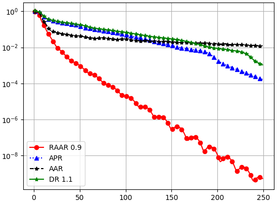
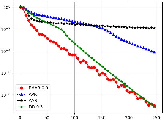
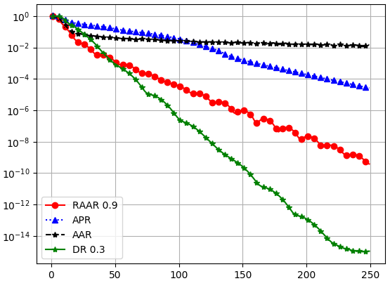
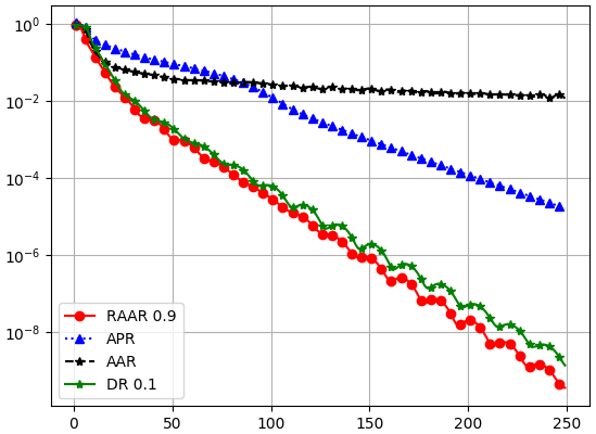
Figure 4 shows the relative error (modulo a constant phase factor) versus iteration of RAAR ( $\beta=0.9$ round-bullet solid line), APR (blue-triangle dotted line), AAR (black-star dashed line) and Gaussian-DRS with (a) $\rho=1.1,$ (b) $\rho=0.5,$ (c) $\rho=0.3$ and (d) $\rho=0.1$ . Note that the AAR, APR and RAAR lines vary slightly across different plots because of random initialization.

The straight-line feature (in all but AAR) in the semi-log plot indicates global geometric convergence. The case with AAR is less clear in Figure 4. But it has been shown that the AAR sequence converges geometrically near the true object (after applying $A^{+}$ ) but converges in power-law ( $\sim k^{-\alpha}$ with $\alpha\in[1,2]$ ) from random initialization [9].

Figure 4 shows that APR outperforms AAR (consistent with the prediction of Corollary 6.4) but underperforms RAAR. By decreasing $\rho$ to either $0.5$ or $0.1$ , the performance of Gaussian-DRS closely matches that of RAAR. The optimal parameter appears to lie between $0.1$ and $0.5$ . For example, with $\rho=0.3,$ Gaussian-DRS significantly outperforms RAAR. The oscillatory behavior of Gaussian-DRS in (d) is due to the dominant complex eigenvalue of $J_{A}$ .

8. Blind ptychography algorithm

In the next two sections we apply the DRS methods to the more challenging problem of blind ptychography. In blind ptychography, we do not assume the full knowledge of the probe which is to be recovered simultaneously with the unknown object.

Let $\nu^{0}$ and $g=\vee_{\mathbf{t}}g^{\mathbf{t}}$ be any pair of the probe and the object estimates producing the same ptychography data as $\mu^{0}$ and $f$ , i.e. the diffraction pattern of $\nu^{\mathbf{t}}\odot g^{\mathbf{t}}$ is identical to that of $\mu^{\mathbf{t}}\odot f^{\mathbf{t}}$ where $\nu^{\mathbf{t}}$ is the $\mathbf{t}$ -shift of $\nu^{0}$ and $g^{\mathbf{t}}$ is the restriction of $g$ to ${\mathcal{M}}^{\mathbf{t}}$ . We refer to the pair $(\nu^{0},g)$ as a blind-ptychographic solution (in the object domain) and $(\mu^{0},f)$ as the true solution.

We can write the total measurement data as $b=|{\mathcal{F}}(\mu^{0},f)|$ where ${\mathcal{F}}$ is the concatenated oversampled Fourier transform acting on $\{\mu^{\mathbf{t}}\odot f^{\mathbf{t}}:\mathbf{t}\in{\mathcal{T}}\}$ (see Appendix A), i.e. a bi-linear transformation in the direct product of the probe space and the object space. By definition, a blind-ptychographic solution $(\nu^{0},g)$ satisfies $|{\mathcal{F}}(\nu^{0},g)|=b$ .

There are two ambiguities inherent to any blind ptychography.

The first is the affine phase ambiguity. Consider the probe and object estimates

(83)		$\displaystyle\nu^{0}({\mathbf{n}})$	$\displaystyle=$	$\displaystyle\mu^{0}({\mathbf{n}})\exp(-{\rm i}a-{\rm i}\mathbf{w}\cdot{\mathbf{n}}),\quad{\mathbf{n}}\in{\mathcal{M}}^{0}$
(84)		$\displaystyle g({\mathbf{n}})$	$\displaystyle=$	$\displaystyle f({\mathbf{n}})\exp({\rm i}b+{\rm i}\mathbf{w}\cdot{\mathbf{n}}),\quad{\mathbf{n}}\in\mathbb{Z}^{2}_{n}$

for any $a,b\in\mathbb{R}$ and $\mathbf{w}\in\mathbb{R}^{2}$ . For any $\mathbf{t}$ , we have the following calculation

$\displaystyle\nu^{\mathbf{t}}({\mathbf{n}})$	$\displaystyle=$	$\displaystyle\nu^{0}({\mathbf{n}}-\mathbf{t})$
	$\displaystyle=$	$\displaystyle\mu^{0}({\mathbf{n}}-\mathbf{t})\exp(-{\rm i}\mathbf{w}\cdot({\mathbf{n}}-\mathbf{t}))\exp(-{\rm i}a)$
	$\displaystyle=$	$\displaystyle\mu^{\mathbf{t}}({\mathbf{n}})\exp(-{\rm i}\mathbf{w}\cdot({\mathbf{n}}-\mathbf{t}))\exp(-{\rm i}a)$

and hence for all ${\mathbf{n}}\in{\mathcal{M}}^{\mathbf{t}},\mathbf{t}\in{\mathcal{T}}$

(85)

\displaystyle\nu^{\mathbf{t}}({\mathbf{n}})g^{\mathbf{t}}({\mathbf{n}})

\displaystyle=

\displaystyle\mu^{\mathbf{t}}({\mathbf{n}})f^{\mathbf{t}}({\mathbf{n}})\exp({\rm i}(b-a))\exp({\rm i}\mathbf{w}\cdot\mathbf{t}).

Clearly, (85) implies that $g$ and $\nu^{0}$ produce the same ptychographic data as $f$ and $\mu^{0}$ since for each $\mathbf{t}$ , $\nu^{\mathbf{t}}\odot g^{\mathbf{t}}$ is a constant phase factor times $\mu^{\mathbf{t}}\odot f^{\mathbf{t}}$ where $\odot$ is the entry-wise (Hadamard) product. It is also clear that the above statement holds true regardless of the set ${\mathcal{T}}$ of shifts and the type of probe.

In addition to the affine phase ambiguity (83)-(84), a scaling factor ( $g=cf,\nu^{0}=c^{-1}\mu^{0},c>0$ ) is inherent to any blind ptychography. Note that when the probe is exactly known (i.e. $\nu^{0}=\mu^{0}$ ), neither ambiguity can occur.

Besides the inherent ambiguities, blind ptychography imposes extra demands on the scanning scheme. For example, there are many other ambiguities inherent to the regular raster scan: ${\mathcal{T}}=\{\mathbf{t}_{kl}={\tau}(k,l):k,l\in\mathbb{Z}\}$ unless the step size $\tau=1$ . Blind ptychography with a raster scan produces $\tau$ -periodic ambiguities called the raster scan pathology as well as non-periodic ambiguities associated with block phase drift. The reader to referred to [17] for a complete analysis of ambiguities associated with the raster scan.

A conceptually simple (though not necessarily the most practical) way to remove these ambiguities is introducing small irregular perturbations to the raster scan with $\tau>m/2$ , i.e. the overlap ratio greater than 50% (see (92) and (93)). For a thorough analysis of the conditions for blind ptychography, we refer the reader to [18, 17].

The basic strategy for blind ptychographic reconstruction is to alternately update the object and probe estimates starting from an initial guess as outlined in Algorithm 1 [51, 50, 19].

1: Input: initial probe guess

\mathbf{\mu}_{1}

and object guess

f_{1}

2: Update the object estimate

\quad f_{k+1}=\arg\min L(A_{k}g)

s.t.

g\in\mathbb{C}^{n\times n}

3: Update the probe estimate

\quad\mu_{k+1}=\arg\min L(B_{k}\nu)

s.t.

\nu\in\mathbb{C}^{m\times m}

4: Terminate if

\||B_{k}\mu_{k+1}|-b\|

stagnates or is less than tolerance; otherwise, go back to step 2 with

k\rightarrow k+1.

Algorithm 1 Alternating minimization (AM)

We solve the inner loops (step 2 and 3 in Algorithm 1) and update the object and probe estimates by the DRS methods where $A_{k}h:={\mathcal{F}}(\mu_{k},h),\forall h\in\mathbb{C}^{n^{2}},$ defines a matrix $A_{k}$ for the $k$ -th probe estimate $\mu_{k}$ and $B_{k}\eta:={\mathcal{F}}(\eta,f_{k+1}),\forall\eta\in\mathbb{C}^{m^{2}},$ for the $(k+1)$ -st image estimate $f_{k+1}$ .

For ease of reference, we denote Algorithm 1 with Gaussian-DRS and Poisson-DRS by Gaussian-DRSAM and Poisson-DRSAM, respectively.

8.1. Initialization

For non-convex iterative optimization, a good initial guess or some regularization is usually crucial for convergence [52, 6]. The initialization step is often glossed over in the development of numerical schemes. This is even more so for blind ptychography which is doubly non-convex because, in addition to the phase retrieval step, extracting the probe and the object from their product is also non-convex.

We say that a probe estimate $\nu^{0}$ satisfies PPC $(\delta)$ (standing for the probe phase constraint) if

(86)

\displaystyle\measuredangle(\nu^{0}({\mathbf{n}}),\mu^{0}({\mathbf{n}}))<\delta\pi,\quad\forall{\mathbf{n}}

where $\delta\in(0,1/2]$ is the uncertainty parameter.

PPC $(\delta)$ defines an alternative measure to the standard norm-based metric. Our default case is $\delta=0.5$ with which PPC is equivalent to $\Re(\bar{\nu}^{0}\odot\mu^{0})>0$ (where the bar denotes the complex conjugate) has the intuitive meaning that at every pixel $\nu^{0}$ and $\mu^{0}$ point to the same half plane in $\mathbb{C}$ (Figure 5).

Our initialization method is inspired by the uniqueness theory in [18] which proves PPC (0.5) is required to remove all other ambiguities than the inherent ones (the affine phase factor and the constant scaling factor).

Under PPC, however, the initial probe may be significantly far away from the true probe in norm. Even if $|\mu_{1}({\mathbf{n}})|=|\mu^{0}({\mathbf{n}})|=\mbox{const.}$ , the probe guess with uniformly distributed $\phi$ in $(-\pi/2,\pi/2]$ has the relative error close to

\sqrt{{1\over\pi}\int^{\pi/2}_{-\pi/2}|e^{{\rm i}\phi}-1|^{2}d\phi}=\sqrt{2(1-{2\over\pi})}\approx 0.8525

with high probability. We use (86) for selecting and quantifying initialization, instead of the usual 2-norm. Non-blind ptychography gives rise to infinitesimally small $\delta$ . In practice, (86) needs only to hold for sufficiently large number of pixels ${\mathbf{n}}$ .

In summary, in our numerical experiments we use the following probe initialization denoted by PPC

(87)

\displaystyle\mu_{1}(\mathbf{n})=\mu^{0}(\mathbf{n})\,\exp{\left[{\rm i}2\pi\frac{\mathbf{k}\cdot\mathbf{n}}{n}\right]}\,\exp{[{\rm i}\phi(\mathbf{n})]},\ \ \ \mathbf{n}\in\mathcal{M}^{0}

where $\phi({\mathbf{n}})$ are independently and uniformly distributed on $(-\pi/2,\pi/2)$ . In our numerical experiments, PPC results in geometric convergence for any ${\mathbf{k}}$ (even though the limiting solution may end up with a different ${\mathbf{k}}$ as allowed by linear phase ambiguity).

9. Numerical experiments for blind ptychography

We test the DRS methods with $\rho=1$ for blind ptychography and demonstrate that even with this far from optimal parameter (cf. Corollary 6.2 and Figure 4), DRSAM converges geometrically under the nearly minimum conditions established in the uniqueness theory [18] (see also Section 8.1 and Section 9.4).

The inner loops of Gaussian DRSAM become

	$\displaystyle u_{k}^{l+1}$	$\displaystyle=$	$\displaystyle\frac{1}{2}u_{k}^{l}+\frac{1}{2}b\odot\mbox{\rm sgn}\big(R_{k}u_{k}^{l}\big)$
	$\displaystyle v_{k}^{l+1}$	$\displaystyle=$	$\displaystyle\frac{1}{2}v_{k}^{l}+\frac{1}{2}b\odot\mbox{\rm sgn}{\Big(S_{k}v_{k}^{l}\Big)}.$

and the inner loops of the Poisson DRSAM become

(88)		$\displaystyle u_{k}^{l+1}$	$\displaystyle=$	$\displaystyle\frac{1}{2}u_{k}^{l}-\frac{1}{3}R_{k}u_{k}^{l}+\frac{1}{6}\mbox{\rm sgn}{\Big(R_{k}u_{k}^{l}\Big)}\odot\sqrt{\|R_{k}u^{l}_{k}\|^{2}+24b^{2}}$
(89)		$\displaystyle v_{k}^{l+1}$	$\displaystyle=$	$\displaystyle\frac{1}{2}v_{k}^{l}-\frac{1}{3}S_{k}v_{k}^{l}+\frac{1}{6}\mbox{\rm sgn}{\Big(S_{k}v_{k}^{l}\Big)}\odot\sqrt{\|S_{k}v_{k}^{l}\|^{2}+24b^{2}}.$

Here $R_{k}=2P_{k}-I$ is the reflector corresponding to the projector $P_{k}:=A_{k}A_{k}^{+}$ and $S_{k}$ is the reflector corresponding to the projector $Q_{k}:=B_{k}B_{k}^{+}$ . We set $u^{1}_{k}=u^{\infty}_{k-1}$ where $u^{\infty}_{k-1}$ is the terminal value at epoch $k-1$ and $v^{1}_{k}=v^{\infty}_{k-1}$ where $v^{\infty}_{k-1}$ is the terminal value at epoch $k-1$ .

9.1. Test objects

In addition to CiB, our second test object is randomly-phased phantom (RPP) defined by $f=P\odot e^{{\rm i}\phi}$ where $P$ is the standard phantom (Fig. 6(a)) and $\{\phi({\mathbf{n}})\}$ are i.i.d. uniform random variables over $[0,2\pi]$ . RPP has the maximal phase range because of its noise-like phase profile. In addition to the huge phase range, RPP has loosely supported parts with respect to the measurement schemes (see below) due to its thick dark margins around the oval.

The third test object is the salted RPP, the sum of RPP and the salt noise (not shown). The salted noise is i.i.d, binomial random variables with probability $0.02$ to be a complex constant in the form of $a(1+{\rm i}),a\in\mathbb{R},$ and probability $0.98$ to be zero. The salt noise reduces the support looseness without significantly changing the original image making the salted RPP more connected with respect to the ptychographic measurement.

9.2. Probe function

We use a randomly phased probe with the unknown transmission function $\mu^{0}({\mathbf{n}})=e^{{\rm i}\theta({\mathbf{n}})}$ where $\theta({\mathbf{n}})$ are random variables. Randomly phased probes have been adopted in ptychographic experiments [42, 39, 46, 49].

We do not explore the issue of varying the probe size in the present work, which was carried out for AAR in [10]. We fix the probe size to $60\times 60$ . In addition to the i.i.d. probe, we consider also correlated probe produced by convolving the i.i.d. probe with characteristic function of the set $\{(k_{1},k_{2})\in\mathbb{Z}^{2}:\max\{|k_{1}|,|k_{2}|\}\leq c\cdot m;\ c\in(0,1]\}$ where the constant $c$ is a measure of the correlation length in the unit of $m=60$ (Fig. 7).

9.3. Error metrics for blind ptychography

We use relative error (RE) and relative residual (RR) as the merit metrics for the recovered image $f_{k}$ and probe $\mu_{k}$ at the $k^{th}$ epoch:

(90)		$\displaystyle\mbox{RE}(k)$	$\displaystyle=$	$\displaystyle\min_{\alpha\in\mathbb{C},\mathbf{r}\in\mathbb{R}^{2}}\frac{\sqrt{\sum_{\mathbf{n}}\|f({\mathbf{n}})-\alpha e^{-{\rm i}{2\pi}\mathbf{n}\cdot\mathbf{r}/n}f_{k}({\mathbf{n}})\|^{2}}}{\\|f\\|}$
(91)		$\displaystyle\mbox{\rm RR}(k)$	$\displaystyle=$	$\displaystyle\frac{\\|b-\|A_{k}f_{k}\|\\|}{\\|b\\|}.$

Note that in (90) both the affine phase and the scaling factors are discounted.

9.4. Sampling schemes

The uniqueness theorem for blind ptychography [17] holds for the following irregularly perturbed raster scans

(92)

\displaystyle\mbox{\rm Rank-one perturbation}\quad\mathbf{t}_{kl}=\tau(k,l)+(\delta^{1}_{k},\delta^{2}_{l}),\quad k,l\in\mathbb{Z}

where $\delta_{k}^{1}$ and $\delta^{2}_{l}$ are small random variables relative to $\tau$ . The other is

(93)

\displaystyle\mbox{\rm Full-rank perturbation}\quad\mathbf{t}_{kl}=\tau(k,l)+(\delta^{1}_{kl},\delta^{2}_{kl}),\quad k,l\in\mathbb{Z}

where $\delta_{kl}^{1}$ and $\delta^{2}_{kl}$ are small random variables relative to $\tau$ . Here the stepsize $\tau<m/2$ corresponding to the overlap ratio greater than $50\%$ . The $50\%$ overlap ratio has been proved to be a nearly minimum requirement for uniqueness with the perturbed raster scans.

We let $\delta_{k}^{1}$ and $\delta^{2}_{l}$ in the rank-one scheme (92) and $\delta_{kl}^{1}$ and $\delta^{2}_{kl}$ in the full-rank scheme (93) to be i.i.d. uniform random variables over $\llbracket-4,4\rrbracket$ . In other words, the adjacent probes overlap by an average of $\tau/m=50\%$ .

9.5. Different combinations

First we compare performance of DRSAM with different combinations of loss functions, scanning schemes and random probes in the case of noiseless measurements with the periodic boundary condition. We use the stopping criteria for the inner loops:

\frac{\||P_{k}u_{k}^{l}|-b\|-\||P_{k}u_{k}^{l+1}|-b\|}{\||P_{k}u_{k}^{l}|-b\|}\leq 10^{-4}

with the maximum number of iterations capped at 60.

Figure 9 shows geometric decay of RE (90) at various rates for the test object CiB. In particular, Fig. 9(a) shows that the full-rank scheme outperforms the rank-one scheme and that Poisson-DRS outperforms (slightly) Gaussian-DRS while Figure 9(b) shows that the i.i.d. probe yields the smallest rate of convergence ( $=0.7562$ ) closely followed by the rate ( $=0.7583$ ) for $c=0.4$ .

9.6. Boundary conditions

The periodic boundary condition conveniently treats all diffraction patterns and object pixels in the same way by assuming that $\mathbb{Z}_{n}^{2}$ is a (discrete) torus. The periodic boundary condition generally forces the slope $\mathbf{r}$ in the affine phase ambiguity to be integers. For 3D blind tomography, however, different linear phase ramps from different projections would collectively create enormous 3D ambiguities that are difficult to make consistent and hence it is highly desirable to remove the linear phase ambiguity early on in the process.

To this end, we consider the non-periodic bright-field boundary conditions taking on some nonzero value in ${\mathcal{M}}\setminus\mathbb{Z}_{n}^{2}$ . We aim to show that the affine phase ambiguity is absent under the bright-field boundary condition.

We test the Poisson-DRSAM with the full-rank scheme with a more stringent error metric

(94)

\displaystyle{\mbox{RE2}}(k)

\displaystyle=

\displaystyle\min_{\theta\in\mathbb{R}}\frac{\|f-e^{{\rm i}\theta}f_{k}\|}{\|f\|}.

We also use the less tolerant stopping rule

\frac{\||P_{k}u_{k}^{l}|-b\|-\||P_{k}u_{k}^{l+1}|-b\|}{\||P_{k}u_{k}^{l}|-b\|}\leq 10^{-5}

for the inner loops with the maximum number of iteration capped at 80.

Fig. 10 demonstrates the capability of the bright-field boundary condition ( $=255$ ) to eliminate the linear phase ambiguity as the stronger error metric (94) decays geometrically before settling down to the final level of accuracy. The final level of accuracy, however, depends on how accurately the inner loops for each epoch are solved. For example, increasing the maximum number of iteration from 80 (Figure 10(a)) to 110 (Figure 10(b)), significantly enhances the final accuracy of reconstruction.

We also see that the bright-field condition enforcement has a better result on RPP than CiB.

9.7. Comparison with rPIE

In this section, we compare the performance of DRSAM in Fig. 10 (a) with that of the regularized PIE (rPIE) [38], the most up-to-date version of ptychographic iterative engine (PIE).

Instead of using all the 64 diffraction patterns simultaneously to update the object and probe estimates, rPIE uses one diffraction pattern at a time in a random order. As such rPIE is analogous to minibatch gradient descent in machine learning. The potential benefits include efficient memory use and a good speed boost by parallel computing resources. Unfortunately, rPIE often fails to converge in the current setting.

To obtain reasonable results for rPIE, we make two adjustments. First, we reduce the phase range of RPP from $(-\pi,\pi]$ to $(-{\pi}/{2},{\pi}/{2}$ ] which is an easier object to reconstruct. Second, for rPIE we use PPC(0.025) for the probe initialization which restricts the probe phase uncertainty to $(-0.025\pi,0.025\pi]$ instead of $(-\pi/2,\pi/2]$ .

There are three adjustable parameters in rPIE and we select these values $\alpha=0.95,\gamma_{\rm prb}=0.95,\gamma_{\rm obj}=0.9$ (see [38] for definition). The order of updating small patches is randomly shuffled in each experiment. For each test image, we run 20 independent experiments and present the best run in Fig. 11. For ease of comparison, Figure 11(b) shows the corresponding results by Gaussian-DRSAM with $\rho=1$ .

9.8. Poisson noise

For noisy measurement, the level of noise is measured in terms of the noise-to-signal ratio (NSR).

{\rm NSR}=\frac{\|b-|Af|\|}{\|Af\|}

where $A$ is the true measurement matrix and $f$ the true object. Because the noise dimension $N$ is roughly 16 times that of the object dimension, the feasibility problem is inconsistent with high probability.

Figure 12 shows RE versus NSR for CiB by Poisson-DRS and Gaussian-DRS with the periodic boundary condition, i.i.d. probe and the full-rank scheme. The maximum number of epoch in DRSAM is limited to $100$ . The RR stabilizes usually after 30 epochs. The (blue) reference straight line has slope = 1. We see that the Gaussian-DRS outperforms the Poisson-DRS, especially when the Poisson RE becomes unstable for NSR $\geq 35\%$ . As noted in [38, 58, 11] fast convergence (with the Poisson log-likelihood function) may introduce noisy artifacts and reduce reconstruction quality.

Most important, Figure 12 confirms that though provably non-convergent in the inconsistent case, Gaussian-DRSAM with $\rho=1$ can yield reasonable solutions under practical termination rules.

10. Conclusion and discussion

We have presented and performed fixed point analysis for DRS methods of phase retrieval and ptychography based on the proximal relaxation of AAR with the relaxation parameter $\rho$ .

For Gaussian-DRS, we have proved that for $\rho\geq 1$ all attracting fixed points must be regular solutions (Theorem 5.2) and that for $\rho\geq 0$ all regular solutions are attracting (Theorem 5.4). In other words, for $\rho\geq 1$ , the problem of stagnation near a non-solutional fixed point, a common problem with AP, is precluded. On the other hand, the problem of divergence (associated with AAR) in the inconsistent case does not arise in view of Theorem 4.6.

In addition, we have given an explicit formula for the optimal parameter $\rho_{*}$ and the optimal rate of convergence in terms of the spectral gap (Corollary 6.2).

When applied to standard phase retrieval with two coded diffraction patterns, Gaussian-DRS converges geometrically from random initialization. When applied to blind ptychography, DRSAM, even with a far from optimal step size, converges geometrically under the nearly minimum conditions established in the uniqueness theory [18]. Our Python codes are posted on https://github.com/AnotherdayBeaux/Blind_-Ptychography_-GUI.

The holy grail of optimization approach has been finding a globally convergent algorithm whose underlying attractors are fixed points. It is worthwhile then to reflect on our results from the global convergence perspective of [33].

We have already pointed out that the analysis in [33] is not applicable to non-differentiable loss functions. As discussed in Section 7, this technical issue has a profound effect on the convergence behavior in the inconsistent case: Gaussian-DRS with $\rho\geq 1$ does not converge, globally or locally. This is an unexpected consequence of Theorem 5.2.

Our numerical experiments with noisy data, however, suggest that non-convergent DRS sequences are nevertheless well-behaved (probably due to hitherto unknown well-controlled attractors) and produce noise-amplification factor of about ${1\over 2}$ when terminated. Analysis of such (possibly strange) attractors and their impacts on numerics is an interesting topic for future research and at the frontier of numerical analysis.

Moreover, the global convergence framework is typically based on the construction of a non-increasing merit function along the iterated sequence (i.e. Lyapunov-like function) that requires the step size (reciprocal of $\rho$ ) to be sufficiently small, resulting in slow convergence in practice.

Nice as it is, perhaps algorithmic convergence should not be our fixation in the case of noisy data. It may be more useful, for numerical purposes, to solve noisy phase retrieval problem by algorithms with non-trivial (non-point-like) attractors which are necessarily non-convergent in the traditional sense.

Appendix A Measurement matrices

Let $\mathbb{Z}_{n}^{2}=\llbracket 0,n-1\rrbracket^{2}$ be the object domain containing the support of the discrete object $f$ where $\llbracket k,l\rrbracket$ denotes the integers between, and including, $k\leq l\in\mathbb{Z}$ . Let ${\mathcal{M}}^{0}:=\mathbb{Z}_{m}^{2},m<n,$ be the initial probe area, i.e. the support of the probe $\mu^{0}$ describing the illumination field.

Let ${\mathcal{T}}$ be the set of all shifts, including $(0,0)$ , involved in the ptychographic measurement. Denote by $\mu^{\mathbf{t}}$ the $\mathbf{t}$ -shifted probe for all $\mathbf{t}\in{\mathcal{T}}$ and ${\mathcal{M}}^{\mathbf{t}}$ the domain of $\mu^{\mathbf{t}}$ . Let $f^{\mathbf{t}}$ the object restricted to ${\mathcal{M}}^{\mathbf{t}}$ . We refer to each $f^{\mathbf{t}}$ as a part of $f$ and write $f=\vee_{\mathbf{t}}f^{\mathbf{t}}$ where $\vee$ is the “union” of functions consistent over their common support set. In ptychography, the original object is broken up into a set of overlapping object parts, each of which produces a $\mu^{\mathbf{t}}$ -coded diffraction pattern. The totality of the coded diffraction patterns is called the ptychographic measurement data. For convenience, we assume the value zero for $\mu^{\mathbf{t}},f^{\mathbf{t}}$ outside of ${\mathcal{M}}^{\mathbf{t}}$ and the periodic boundary condition on $\mathbb{Z}_{n}^{2}$ when $\mu^{\mathbf{t}}$ crosses over the boundary of $\mathbb{Z}_{n}^{2}$ .

Let the $\mu$ -Fourier transform of $f^{0}$ be written as

F^{0}(\mathbf{w})=\sum_{{\mathbf{k}}\in{\mathcal{M}}^{0}}e^{-{\rm i}2\pi{\mathbf{k}}\cdot\mathbf{w}}\mu^{0}({\mathbf{k}})f^{0}({\mathbf{k}}),\quad\mathbf{w}=(w_{1},w_{2})\in[0,1]^{2}.

and the $\mu$ -coded diffraction pattern as

(95)

\displaystyle|F^{0}(\mathbf{w})|^{2}=\sum_{{\mathbf{k}}\in\widetilde{\mathcal{M}}^{0}}\left\{\sum_{{\mathbf{k}}^{\prime}\in{\mathcal{M}}^{0}}\mu^{0}({\mathbf{k}}+{\mathbf{k}}^{\prime})f^{0}({\mathbf{k}}^{\prime}+{\mathbf{k}})\overline{\mu^{0}({\mathbf{k}}^{\prime})f^{0}({\mathbf{k}}^{\prime})}\right\}e^{-{\rm i}2\pi{\mathbf{k}}\cdot\mathbf{w}}

where

\widetilde{\mathcal{M}}^{0}=\{(k_{1},k_{2})\in\mathbb{Z}^{2}:-m+1\leq k_{1}\leq m-1,-m+1\leq k_{2}\leq m-1\}.

Here and below the over-line notation means complex conjugacy. In view of (96), we sample the coded diffraction pattern on the grid

(96)

\displaystyle L=\Big\{(w_{1},w_{2})\ |\ w_{j}=0,\frac{1}{2m-1},\frac{2}{2m-1},\ldots,\frac{2m-2}{2m-1}\Big\}.

We assume randomness in the phases $\theta$ of the mask function $\mu^{0}({\mathbf{n}})=|\mu^{0}|({\mathbf{n}})e^{{\rm i}\theta({\mathbf{n}})}$ where $\theta({\mathbf{n}})$ are independent, continuous real-valued random variables over $[0,2\pi)$ . We also require that $|\mu^{0}|({\mathbf{n}})\neq 0,\forall{\mathbf{n}}\in{\mathcal{M}}^{0}$ .

Let ${\mathcal{F}}(\nu^{0},g)$ be the bilinear transformation representing the totality of the Fourier (magnitude and phase) data for any probe $\nu$ and object $g$ . From ${\mathcal{F}}(\nu^{0},g)$ we can define two measurement matrices. First, for a given $\nu^{0}\in\mathbb{C}^{m^{2}}$ , let $A_{\nu}$ be defined via the relation $A_{v}g:={\mathcal{F}}(\nu^{0},g)$ for all $g\in\mathbb{C}^{n^{2}}$ ; second, for a given $g\in\mathbb{C}^{n^{2}}$ , let $B_{g}$ be defined via $B_{g}\nu={\mathcal{F}}(\nu^{0},g)$ for all $\nu^{0}\in\mathbb{C}^{m^{2}}$ .

More specifically, let $\Phi$ denote the $L$ -sampled Fourier matrix. The measurement matrix $A_{\nu}$ is a concatenation of $\{\Phi\,\hbox{\rm diag}(\nu^{\mathbf{t}}):\mathbf{t}\in{\mathcal{T}}\}$ (Figure (13)(a)). Likewise, $B_{g}$ is $\{\Phi\,\hbox{\rm diag}(g^{\mathbf{t}}):\mathbf{t}\in{\mathcal{T}}\}$ stacked on top of each other (Figure (13)(b)). Since $\Phi$ has orthogonal columns, both $A_{\nu}$ and $B_{g}$ have orthogonal columns and their pseudo-inverses are efficient to compute.

We simplify the notation by setting $A=A_{\mu}$ and $B=B_{f}$ .

Appendix B The Poisson versus Gaussian log-likelihood functions

Consider the Poisson distribution

P(n)={\lambda^{n}e^{-\lambda}\over n!}

Let $n=\lambda(1+\epsilon)$ where $\lambda\gg 1$ and $\epsilon\ll 1$ . Using Stirling’s formula

n!\sim\sqrt{2\pi n}e^{-n}n^{n}

in the Poisson distribution, we obtain

	$\displaystyle P(n)$	$\displaystyle\sim$	$\displaystyle{\lambda^{\lambda(1+\epsilon)}e^{-\lambda}\over\sqrt{2\pi}e^{-\lambda(1+\epsilon)}[\lambda(1+\epsilon)]^{\lambda(1+\epsilon)+1/2}}$
		$\displaystyle\sim$	$\displaystyle{1\over\sqrt{2\pi\lambda}e^{-\lambda\epsilon}(1+\epsilon)^{\lambda(1+\epsilon)+1/2}}.$

By the asymptotic

(1+\epsilon)^{\lambda(1+\epsilon)+1/2}\sim e^{\lambda\epsilon+\lambda\epsilon^{2}/2}

we have

(97)

\displaystyle P(n)\sim{e^{-\lambda\epsilon^{2}/2}\over\sqrt{2\pi\lambda}}={e^{-(n-\lambda)^{2}/(2\lambda)}\over\sqrt{2\pi\lambda}}.

Namely in the low noise limit the Poisson noise is equivalent to the Gaussian noise of the mean $|Af|^{2}$ and the variance equal to the intensity of the diffraction pattern. The overall SNR can be tuned by varying the signal energy $\|Af\|^{2}$ .

The negative log-likelihood function for the right hand side of (97) is

(98)

\displaystyle\sum_{j}\ln|u[j]|+{1\over 2}\left|{b[j]\over|u[j]|}-|u[j]|\right|^{2},\quad b=\mbox{noisy diffraction pattern.}

For small NSR and in the vicinity of $b$ , we make the substitution

{\sqrt{b[j]}\over|u[j]|}\to 1,\quad\ln|u[j]|\to\ln\sqrt{b[j]}

to obtain

(99)

\displaystyle\mbox{const.}+{1\over 2}\sum_{j}\left|\sqrt{b[j]}-|u[j]|\right|^{2}.

Appendix C Equivalence between DRS and ADMM

We show that ADMM applied to the augmented Lagrangian

(100)

\displaystyle{\mathcal{L}}(y,z)=K(y)+L(z)+\lambda^{*}(z-y)+{\rho\over 2}\|z-y\|^{2}

in the order alternatively as

(101)	$\displaystyle z_{k+1}$	$\displaystyle=$	$\displaystyle\arg\min_{z}{\mathcal{L}}(y_{k+1},z,\lambda_{k})$
(102)	$\displaystyle y_{k+1}$	$\displaystyle=$	$\displaystyle\arg\min_{x}{\mathcal{L}}(y,z_{k},\lambda_{k})$
(103)	$\displaystyle\lambda_{k+1}$	$\displaystyle=$	$\displaystyle\lambda_{k}+\rho(z_{k+1}-y_{k+1}).$

is equivalent to DRS.

Let

(104)		$\displaystyle z_{k+1}$	$\displaystyle=$	$\displaystyle\arg\min_{z}{\mathcal{L}}(y_{k},z,\lambda_{k})=\hbox{prox}_{L/\rho}(y_{k}-\lambda_{k}/\rho)$
(105)		$\displaystyle y_{k+1}$	$\displaystyle=$	$\displaystyle\arg\min_{x}{\mathcal{L}}(y,z_{k+1},\lambda_{k})=\hbox{prox}_{K/\rho}(z_{k+1}+\lambda_{k}/\rho)$

and consider the new variable

u_{k}:=z_{k}+\lambda_{k-1}/\rho.

We have from (103) that

\displaystyle u_{k+1}=y_{k+1}+\lambda_{k+1}/\rho.

By (105), we also have

y_{k+1}=P_{X}(z_{k+1}+\lambda_{k}/\rho)=P_{X}u_{k+1}

and

\displaystyle y_{k}-\lambda_{k}/\rho=2y_{k}-u_{k}=R_{X}u_{k}.

So (104) becomes

(106)

\displaystyle z_{k+1}=\hbox{prox}_{L/\rho}(R_{X}u_{k}).

Note also that by (103)

\displaystyle u_{k}-P_{X}u_{k}=\lambda_{k}/\rho

and hence

\displaystyle u_{k+1}=z_{k+1}+\lambda_{k}/\rho=u_{k}-P_{X}u_{k}+\hbox{prox}_{L/\rho}(R_{X}u_{k})

which is exactly the DRS scheme (29) after rearrangement.

Appendix D Perturbation analysis of Poisson-DRS

The full analysis of the Poisson-DRS (30) is more challenging. Instead, we give a perturbative derivation of analogous result to Theorem 4.6 for the Poisson-DRS with small positive $\rho$ .

For small $\rho$ , by keeping only the terms up to ${\mathcal{O}}(\rho)$ we obtain the perturbed DRS:

(107)

\displaystyle u_{k+1}={1\over 2}u_{k}-{1\over 2}(1-{\rho\over 2})R_{X}u_{k}+P_{Y}R_{X}u_{k}.

Writing

I=P_{X}+P^{\perp}_{X}\quad\mbox{and}\quad R_{X}=P_{X}-P^{\perp}_{X},

we then have the estimates

	$\displaystyle\\|u_{k+1}\\|$	$\displaystyle\leq$	$\displaystyle\\|{\rho\over 4}P_{X}u_{k}+(1-{\rho\over 4})P^{\perp}_{X}u_{k}\\|+\\|P_{Y}R_{X}u_{k}\\|$
		$\displaystyle\leq$	$\displaystyle(1-{\rho\over 4})\\|u_{k}\\|+\\|b\\|$

since $\rho$ is small. Iterating this bound, we obtain

\displaystyle\|u_{k+1}\|\leq(1-{\rho\over 4})^{k}\|u_{1}\|+\|b\|\sum_{j=0}^{k-1}(1-{\rho\over 4})^{j}

and hence

(108)

\displaystyle\limsup_{k\to\infty}\|u_{k}\|\leq{4\over\rho}\|b\|.

Note that the small $\rho$ limit and the Poisson-to-Gaussian limit in Appendix B do not commune, resulting in a different constant in (108) from Theorem 4.6.

Appendix E Eigen-structure

The vector space $\mathbb{C}^{N}=\mathbb{R}^{N}\oplus_{\mathbb{R}}i\mathbb{R}^{N}$ is isomorphic to $\mathbb{R}^{2N}$ via the map

V(v):=\left[\begin{array}[]{c}\Re(v)\\ \Im(v)\end{array}\right],\quad\forall v\in\mathbb{C}^{N}

and endowed with the real inner product

\langle u,v\rangle:=\Re(u^{*}v)=V(u)^{\top}V(v),\quad u,v\in\mathbb{C}^{N}.

We have

(109)

\displaystyle V(H\xi)=\left[\begin{matrix}\Re[H]\Re[\xi]+\Im[H]\Im[\xi]\\ \Re[H]\Im[\xi]-\Im[H]\Re[\xi]\end{matrix}\right]=\left[\begin{matrix}{\mathcal{H}}^{\top}V(\xi)\\ {\mathcal{H}}^{\top}V(-{\rm i}\xi)\end{matrix}\right],\quad\xi\in\mathbb{C}^{n}.

Let $\lambda_{1}\geq\lambda_{2}\geq\cdots\geq\lambda_{2n}\geq\lambda_{2n+1}=\cdots=\lambda_{N}=0$ be the singular values of ${\mathcal{H}}$ in (63) with the corresponding right singular vectors $\{\eta_{k}\in\mathbb{R}^{N}\}_{k=1}^{N}$ and left singular vectors $\{{\xi}_{k}\in\mathbb{R}^{2n}\}_{k=1}^{2n}$ . By definition, for $k=1,\ldots,2n$ ,

(110)		$\displaystyle H^{*}\eta_{k}$	$\displaystyle=$	$\displaystyle\lambda_{k}G^{-1}(\xi_{k}),$
(111)		$\displaystyle\Re[HG^{-1}(\xi_{k})]$	$\displaystyle=$	$\displaystyle\lambda_{k}\eta_{k}.$

Proposition E.1.

We have $\xi_{1}=V(f)$ , $\xi_{2n^{2}}=V(-{\rm i}f)$ , $\lambda_{1}=1,\lambda_{2n^{2}}=0$ as well as $\eta_{1}=|Af|$ .

Proof.

Since

\displaystyle Hf=\Omega^{*}Af=|Af|

we have by (109)

(112)

\displaystyle\Re[Hf]={\mathcal{H}}^{\top}\xi_{1}=|Af|,\quad\Im[Hf]={\mathcal{H}}^{\top}\xi_{2n^{2}}=0

and hence the results. ∎

Corollary E.2.

(113)		$\displaystyle\lambda_{2}$	$\displaystyle=$	$\displaystyle\max\{\\|\Im(Hu)\\|:{u\in\mathbb{C}^{n},u\perp{\rm i}f,\\|u\\|=1}\}$
(113)			$\displaystyle=$	$\displaystyle\max\{\\|{\mathcal{H}}^{\top}u\\|:{u\in\mathbb{R}^{2n^{2}},u\perp\xi_{1},\\|u\\|=1}\}$

Proof.

By (109),

\Im[Hu]={\mathcal{H}}^{\top}V(-{\rm i}u).

The orthogonality condition ${\rm i}u\perp f$ is equivalent to

V(x_{0})\perp V(-{\rm i}u).

Hence, by Proposition E.1 $\xi_{2}$ is the maximizer of the right hand side of (113), yielding the desired value $\lambda_{2}$ .

∎

Proposition E.3.

For $k=1,\ldots,2n^{2}$ ,

(114)

\displaystyle\lambda_{k}^{2}+\lambda_{2n^{2}+1-k}^{2}=1

(115)		$\displaystyle\xi_{2n^{2}+1-k}$	$\displaystyle=$	$\displaystyle V(-{\rm i}V^{-1}(\xi_{k}))$
(116)		$\displaystyle\xi_{k}$	$\displaystyle=$	$\displaystyle V({\rm i}V^{-1}(\xi_{2n^{2}+1-k})).$

Proof.

Since $H$ is an isometry, we have $\|w\|=\|Hw\|,\forall w\in\mathbb{C}^{n}$ . On the other hand, we have

\displaystyle\|Hw\|^{2}=\|V(Hw)\|^{2}=\|{\mathcal{H}}^{\top}V(w)\|^{2}+\|{\mathcal{H}}^{\top}V(-{\rm i}w)\|^{2}\ldots

and hence

(117)

\displaystyle\|V(w)\|^{2}=\|{\mathcal{H}}^{\top}V(w)\|^{2}+\|{\mathcal{H}}^{\top}V(-{\rm i}w)\|^{2}.

Now we prove (114), (115) and (116) by induction.

Recall the variational characterization of the singular values/vectors

(118)

\displaystyle\lambda_{j}=\max\|{\mathcal{H}}^{\top}{u}\|,

\displaystyle\xi_{j}=\hbox{\rm arg}\max\|{\mathcal{H}}^{\top}{u}\|,

\displaystyle\hbox{s.t.}\,\,{u}\perp{\xi}_{1},\ldots,{\xi}_{j-1},\quad\|u\|=1

By Proposition E.1, (114), (115) and (116) hold for $k=1$ . Suppose (114), (115) and (116) hold for $k=1,\ldots,j-1$ and we now show that they also hold for $k=j$ .

Hence by (117)

\lambda^{2}_{j}=\max_{\|u\|=1}\|{\mathcal{H}}^{\top}{u}\|^{2}=1-\min_{\|v\|=1}\|{\mathcal{H}}^{\top}{v}\|^{2},\quad\hbox{s.t.}\,\,{u}\perp{\xi}_{1},\ldots,{\xi}_{j-1},\quad v=V(-{\rm i}V^{-1}(u)).

The condition ${u}\perp{\xi}_{1},\ldots,{\xi}_{j-1}$ implies $v\perp{\xi}_{2n^{2}},\ldots,{\xi}_{2n^{2}+2-j}$ and vice versa. By the dual variational characterization to (118)

\displaystyle\lambda_{2n^{2}+1-j}=\min\|{\mathcal{H}}^{\top}{u}\|,

\displaystyle\xi_{2n^{2}+1-j}=\hbox{\rm arg}\min\|{\mathcal{H}}^{\top}{u}\|,

\displaystyle\hbox{s.t.}\,\,{u}\perp{\xi}_{2n^{2}},\ldots,{\xi}_{2n^{2}+2-j},\|u\|=1,

we have

\lambda_{j}^{2}=1-\lambda_{2n^{2}+1-j}^{2},\quad\xi_{2n^{2}+1-j}=V(-{\rm i}V^{-1}(\xi_{j})).

∎

Proposition E.4.

For each $k=1,\ldots,2n^{2}$ ,

(119)		$\displaystyle HH^{*}\eta_{k}=\lambda_{k}(\lambda_{k}\eta_{k}+{\rm i}\lambda_{2n^{2}+1-k}\eta_{2n^{2}+1-k}),$
(120)		$\displaystyle HH^{*}\eta_{2n^{2}+1-k}=\lambda_{2n^{2}+1-k}(\lambda_{2n^{2}+1-k}\eta_{2n^{2}+1-k}-{\rm i}\lambda_{k}\eta_{k})$

implying

\displaystyle HH^{*}

\displaystyle=

\displaystyle\left[\begin{matrix}\lambda_{k}^{2}&\lambda_{k}\lambda_{2n^{2}+1-k}\\ \lambda_{k}\lambda_{2n^{2}+1-k}&\lambda_{2n^{2}+1-k}^{2}\end{matrix}\right]

in the basis of $\eta_{k},{\rm i}\eta_{2n^{2}+1-k}$ .

Proof.

By definition, ${\mathcal{H}}\eta_{k}=\lambda_{k}{\xi}_{k}.$ Hence

H^{*}\eta_{k}=(\Re[H^{*}]+{\rm i}\Im[H^{*}])\eta_{k}=\lambda_{k}(\xi_{k}^{\rm R}+{\rm i}\xi_{k}^{\rm I})

where

\xi_{k}=\left[\begin{matrix}\xi_{k}^{\rm R}\\ \xi_{k}^{\rm I}\end{matrix}\right],\quad\xi_{k}^{\rm R},\xi_{k}^{\rm I}\in\mathbb{R}^{n}.

On the other hand, ${\mathcal{H}}^{\top}\xi_{k}=\lambda_{k}\eta_{k}$ and hence

(121)

\displaystyle\Re[H]\xi_{k}^{\rm R}-\Im[H]\xi_{k}^{\rm I}=\lambda_{k}\eta_{k}.

Now we compute $HH^{*}\eta_{k}$ as follows.

(122)	$\displaystyle HH^{*}\eta_{k}$	$\displaystyle=$	$\displaystyle\lambda_{k}H(\xi_{k}^{\rm R}+{\rm i}\xi_{k}^{\rm I})$
		$\displaystyle=$	$\displaystyle\lambda_{k}(\Re[H]+{\rm i}\Im[H])(\xi_{k}^{\rm R}+{\rm i}\xi_{k}^{\rm I})$
		$\displaystyle=$	$\displaystyle\lambda_{k}(\Re[H]\xi_{k}^{\rm R}-\Im[H]\xi_{k}^{\rm I})+{\rm i}\lambda_{k}(\Re[H]\xi_{k}^{\rm I}+\Im[H]\xi_{k}^{\rm R})$
		$\displaystyle=$	$\displaystyle\lambda_{k}^{2}\eta_{k}+{\rm i}\lambda_{k}(\Re[H]\xi_{k}^{\rm I}+\Im[H]\xi_{k}^{\rm R})$

by (121).

Notice that

(123)	$\displaystyle\Re(H)\xi_{k}^{\rm I}+\Im(H)\xi_{k}^{\rm R}$	$\displaystyle=$	$\displaystyle{\mathcal{H}}^{\top}\left[\begin{matrix}\Re(-{\rm i}V^{-1}(\xi_{k}))\\ \Im(-{\rm i}V^{-1}(\xi_{k}))\end{matrix}\right]$
		$\displaystyle=$	$\displaystyle{\mathcal{H}}^{\top}V(-{\rm i}V^{-1}(\xi_{k}))$
		$\displaystyle=$	$\displaystyle{\mathcal{H}}^{\top}\xi_{2n^{2}+1-k}$
		$\displaystyle=$	$\displaystyle\lambda_{2n^{2}+1-k}\eta_{2n^{2}+1-k}$

by Proposition E.3.

Putting (122) and (123) together, we have (119). Likewise, (120) follows from a similar calculation. ∎

Acknowledgment

This research is supported by the US National Science Foundation grant DMS-1413373 and SIMONS FDN 2019-24. A.F. thanks National Center for Theoretical Sciences (NCTS), Taiwan, where the present work was carried out, for the hospitality during his visits in June and August 2018.

References

[1] H. H. Bauschke & J. M. Borwein, On projection algorithms for solving convex feasibility problems, SIAM Rev. 38 (1996) 367-426.
[2] H.H. Bauschkea, J.Y. B. Cruz, T.T.A. Nghia, H.M. Phan & X. Wang, The rate of linear convergence of the Douglas-Rachford algorithm for subspaces is the cosine of the Friedrichs angle, J. Approx. Theory 185 (2014) 63-79.
[3] H.H. Bauschke, P.L. Combettes and D. R. Luke, Phase retrieval, error reduction algorithm, and Fienup variants: a view from convex optimization, J. Opt. Soc. Am. A 19 (2002) 13341-1345.
[4] H.H. Bauschke, P.L. Combettes and D. R. Luke, Hybrid projection-reflection method for phase retrieval, J. Opt. Soc. Am. A 20 (2003) 1025-1034.
[5] H. H. Bauschke, P. L. Combettes and D. R. Luke, Finding best approximation pairs relative to two closed convex sets in Hilbert space, J. Approx. Theory 127 (2004) 178-192.
[6] L. Bian, J. Suo, J. Chung, X. Ou, C. Yang, F. Chen and Q. Dai, Fourier ptychographic reconstruction using Poisson maximum likelihood and truncated Wirtinger gradient, Sci. Rep. 6 (2016), 27384.
[7] O. Bunk, M. Dierolf, S. Kynde, I. Johnson, O. Marti & F. Pfeiffer, Influence of the overlap parameter on the convergence of the ptychographical iterative engine, Ultramicroscopy 108 (2008) 481-487.
[8] H. Chang, P. Enfedaque and S. Marchesini, Blind ptychographic phase retrieval via convergent alternating direction method of multipliers, SIAM J. Imaging Sci. 12 (2019) 153-185.
[9] P. Chen and A. Fannjiang, Phase retrieval with a single mask by Douglas-Rachford algorithms, Appl. Comput. Harmon. Anal. 44 (2018), 665-699.
[10] P. Chen and A. Fannjiang, Coded-aperture ptychography: uniqueness and reconstruction, Inverse Problems 34 (2018) 025003.
[11] P. Chen, A. Fannjiang and G. Liu, Phase retrieval with one or two coded diffraction patterns by alternating projection with the null initialization, J. Fourier Anal. Appl. 24 (2018), 719-758.
[12] M. Dierolf, A. Menzel, P. Thibault, P. Schneider, C. M. Kewish, R. Wepf, O. Bunk, and F. Pfeiffer, Ptychographic x-ray computed tomography at the nanoscale, Nature 467 (2010), 436-439.
[13] J. Douglas and H.H. Rachford, On the numerical solution of heat conduction problems in two and three space variables, Trans. Am. Math. Soc. 82 (1956), 421-439.
[14] J. Eckstein and D.P. Bertsekas, On the Douglas-Rachford splitting method and the proximal point algorithm for maximal monotone operators, Math. Program. A 55 (1992), 293-318.
[15] V. Elser, Phase retrieval by iterated projections, J. Opt. Soc. Am. A 20 (2003), 40-55.
[16] A. Fannjiang, Absolute uniqueness of phase retrieval with random illumination, Inverse Problems 28 (2012), 075008.
[17] A. Fannjiang, Raster grid pathology and the cure, Multiscale Model. Simul. 17 (2019), 973-995.
[18] A. Fannjiang & P. Chen, Blind ptychography: uniqueness and ambiguities, Inverse Problems to appear.
[19] A. Fannjiang and W. Liao, Fourier phasing with phase-uncertain mask, Inverse Problems 29 (2013) 125001.
[20] A. Fannjiang and Z. Zhang, Blind ptychography by Douglas-Rachford splitting, arxiv:1809.00962.
[21] H.M.L. Faulkner and J.M. Rodenburg, Movable aperture lensless transmission microscopy: A novel phase retrieval algorithm, Phys. Rev. Lett. 93 (2004), 023903.
[22] H.M.L. Faulkner and J.M. Rodenburg, Error tolerance of an iterative phase retrieval algorithm for moveable illumination microscopy, Ultramicroscopy 103:2 (2005), 153-164.
[23] J.R. Fienup, Phase retrieval algorithms—a comparison, Appl. Opt. 21, 2758-2769 (1982).
[24] J.R. Fienup, C.C. Wackerman, Phase-retrieval stagnation problems and solutions, J. Opt. Soc. Am. A 3 (1986) 1897-1907.
[25] D. Gabay and B. Mercier, A dual algorithm for the solution of nonlinear variational problems via finite element approximation, Computers & Mathematics with Applications 2 (1976), 17-40.
[26] P. Giselsson and S. Boyd, Linear convergence and metric selection for Douglas-Rachford Splitting and ADMM, IEEE Trans. Auto. Control 62:2(2017) 532-544.
[27] R. Glowinski and A. Marroco, Sur l’approximation, par éléments finis d’ordre un, et la résolution, par pénalisation-dualité d’une classe de problémes de dirichlet non linéaires, ESAIM: Mathematical Modelling and Numerical Analysis, 9(1975), 41-76.
[28] P. Godard, M. Allain, V. Chamard, and J. Rodenburg, Noise models for low counting rate coherent diffraction imaging, Opt. Express 20 (2012), 25914-25934.
[29] B. He and X. Yuan, On the ${\mathcal{O}}(1/m)$ convergence rate of the Douglas-Rachford alternating direction method, SIAM J. Numer. Anal. 50 (2012) 700-709.
[30] R. Hesse, D. R. Luke, S. Sabach, and M.K. Tam, Proximal heterogeneous block implicit-explicit method and application to blind ptychographic diffraction imaging, SIAM J. Imag. Sci. 8 (2015) pp. 426-457.
[31] A.P. Konijnenberg, W.M.J. Coene and H.P. Urbach, Model-independent noise-robust extension of ptychography, Opt. Exp. 26 (2018) 5857-5874.
[32] C. Kuang, Y. Ma, R. Zhou, J. Lee, G. Barbastathis, R. R. Dasari, Z. Yaqoob & P.T.C. So, Digital micromirror device-based laser-illumination Fourier ptychographic microscopy, Opt. Exp. 23(2015), 26999-27010.
[33] G. Li & T. K. Pong, Douglas-Rachford splitting for nonconvex optimization with application to nonconvex feasibility problems, Math. Program. A 159 (2016), 371-401
[34] J. Li and T. Zhou, On relaxed averaged alternating reflections (RAAR) algorithm for phase retrieval with structured illumination, Inverse Problems 33 (2017) 025012.
[35] P.-L. Lions and B. Mercier, Splitting algorithms for the sum of two nonlinear operators, SIAM J. Num. Anal. 16 (1979), 964-979.
[36] D. Luke, Relaxed averaged alternating reflections for diffraction imaging, Inverse Probl. 21 (2005) 37-50.
[37] D. Luke, Finding best approximation pairs relative to a convex and prox-regular set in a Hilbert space, SIAM J. Optim. 19 (2008) 714-739.
[38] A. M. Maiden, D. Johnson and P. Li, Further improvements to the ptychographical iterative engine, Optica 4 (2017), 736-745.
[39] A.M. Maiden, G.R. Morrison, B. Kaulich, A. Gianoncelli & J.M. Rodenburg, Soft X-ray spectromicroscopy using ptychography with randomly phased illumination, Nat. Commun. 4 (2013), 1669.
[40] A.M. Maiden & J.M. Rodenburg, An improved ptychographical phase retrieval algorithm for diffractive imaging, Ultramicroscopy 109 (2009), 1256-1262.
[41] S. Marchesini, H. Krishnan, B. J. Daurer, D. A. Shapiro, T. Perciano, J. A. Sethian, and F. R. Maia, SHARP: a distributed GPU-based ptychographic solver, J. Appl. Crystallogr. 49 (2016), 1245-1252.
[42] G.R. Morrison, F. Zhang, A. Gianoncelli and I.K. Robinson, X-ray ptychography using randomized zone plates, Opt. Exp. 26 (2018) 14915-14927.
[43] Y. S. G. Nashed, D. J. Vine, T. Peterka, J. Deng, R. Ross and C. Jacobsen, Parallel ptychographic reconstruction, Opt. Express 22 (2014) 32082-32097.
[44] K.A. Nugent, Coherent methods in the X-ray sciences, Adv. Phys. 59 (2010) 1-99.
[45] X. Ou, G. Zheng and C. Yang, Embedded pupil function recovery for Fourier ptychographic microscopy, Opt. Exp. 22 (2014) 4960-4972.
[46] X. Peng, G.J. Ruane, M.B. Quadrelli & G.A. Swartzlander, Randomized apertures: high resolution imaging in far field, Opt. Express 25 (2017) 296187.
[47] F. Pfeiffer, X-ray ptychography, Nat. Photon. 12 (2017) 9-17.
[48] J.M. Rodenburg and H.M.L. Faulkner, A phase retrieval algorithm for shifting illumination, Appl. Phys. Lett. 85 (2004), 4795.
[49] M. Stockmar, P. Cloetens, I. Zanette, B. Enders, M. Dierolf, F. Pfeiffer, and P. Thibault, Near-field ptychography: phase retrieval for inline holography using a structured illumination, Sci. Rep. 3 (2013), 1927.
[50] P. Thibault, M. Dierolf, O. Bunk, A. Menzel & F. Pfeiffer, Probe retrieval in ptychographic coherent diffractive imaging, Ultramicroscopy 109 (2009), 338-343.
[51] P. Thibault, M. Dierolf, A. Menzel, O. Bunk, C. David and F. Pfeiffer, High-resolution scanning X-ray diffraction microscopy, Science 321 (2008), 379-382.
[52] P. Thibault and M. Guizar-Sicairos, Maximum-likelihood refinement for coherent diffractive imaging, New J. Phys. 14 (2012), 063004.
[53] L. Tian, Z. Liu, L-H Yeh, M. Chen, J. Zhong & L. Waller, Computational illumination for high-speed in vitro Fourier ptychographic microscopy, Optica 2 (2015) 904-911.
[54] Z. Wen, C. Yang, X. Liu and S. Marchesini, Alternating direction methods for classical and ptychographic phase retrieval, Inverse Problems 28 (2012), 115010.
[55] L. Yeh, J. Dong, J. Zhong, L.Tian, M. Chen, G. Tang, M. Soltanolkotabi, and L. Waller, Experimental robustness of Fourier ptychography phase retrieval algorithms, Optics Express 23 (2015) 33214-33240.
[56] Y. Zhang, P. Song, Q. Dai, Fourier ptychographic microscopy using a generalized Anscombe transform approximation of the mixed Poisson-Gaussian likelihood, Opt. Exp. 25 (2017) 168-179.
[57] G. Zheng, R. Horstmeyer and C.Yang, Wide-field, high-resolution Fourier ptychographic microscopy, Nature Photonics 7 (2013), 739-745.
[58] C. Zuo, J. Sun and Q. Chen, Adaptive step-size strategy for noise-robust Fourier ptychographic microscopy, Optics Express 24 (2016), 20724-20744.

$\displaystyle\\|b\\|^{2}$	$\displaystyle=$	$\displaystyle\\|\tilde{P}_{X}b\\|^{2}+\\|\tilde{P}^{\perp}_{X}b\\|^{2}$
	$\displaystyle=$	$\displaystyle\left\\|{\rho\|x\|\over 1+\rho}+{b\over 1+\rho}\right\\|^{2}+\left\\|{\rho\over 1+\rho}(\|b\|-\|x\|)\right\\|^{2}$
	$\displaystyle=$	$\displaystyle{2\rho^{2}\over(\rho+1)^{2}}\\|x\\|^{2}+{2\rho(1-\rho)\over(\rho+1)^{2}}\|x\|\cdot b+{\rho^{2}+1\over(\rho+1)^{2}}\\|b\\|^{2}$

	$\displaystyle\left\\|{b^{2}\over\|x\|}\right\\|$	$\displaystyle>$	$\displaystyle{\\|b\\|^{2}\over\\|x\\|}$
	$\displaystyle{b\over\|x\|}\cdot b^{2}$	$\displaystyle=$	$\displaystyle\left\\|{b^{3/2}\over\|x\|^{1/2}}\right\\|^{2}>{\\|b\\|^{4}\over\\|\|x\|^{1/2}\odot b^{1/2}\\|^{2}}={\\|b\\|^{4}\over\|x\|\cdot b}.$

Fixed Point Analysis of Douglas-Rachford Splitting for Ptychography and Phase RetrievalThanks: ∗Corresponding author: fannjiang@math.ucdavis.eduThanks: SIAM Journal on Imaging Sciences (2020)

Abstract.

1. Introduction

2. Averaged Alternating Reflections (AAR)

Proposition 2.1.

2.1. Phase retrieval as feasibility

Proposition 2.2.

3. Douglas-Rachford Splitting (DRS)

4. Fixed points

Proposition 4.1.

Proof.

Proposition 4.2.

Proof.

Proposition 4.3.

Proof.

Proposition 4.4.

Proof.

Proposition 4.5.

Theorem 4.6.

Proof.

Corollary 4.7.

Proof.

5. Stability analysis

Proposition 5.1.

Proof.

Theorem 5.2.

Remark 5.3.

Proof.

Theorem 5.4.

Proof.

6. Spectral gap

Proposition 6.1.

Corollary 6.2.

Remark 6.3.

Proof.

Corollary 6.4.

7. Selection of parameter

7.1. Phase retrieval with noiseless data

8. Blind ptychography algorithm

8.1. Initialization

9. Numerical experiments for blind ptychography

9.1. Test objects

9.2. Probe function

9.3. Error metrics for blind ptychography

9.4. Sampling schemes

9.5. Different combinations

9.6. Boundary conditions

9.7. Comparison with rPIE

9.8. Poisson noise

10. Conclusion and discussion

Appendix A Measurement matrices

Appendix B The Poisson versus Gaussian log-likelihood functions

Appendix C Equivalence between DRS and ADMM

Appendix D Perturbation analysis of Poisson-DRS

Appendix E Eigen-structure

Proposition E.1.

Proof.

Corollary E.2.

Proof.

Proposition E.3.

Proof.

Proposition E.4.

Proof.

Acknowledgment

References

Fixed Point Analysis of Douglas-Rachford Splitting for Ptychography and Phase RetrievalThanks: ^∗Corresponding author: fannjiang@math.ucdavis.eduThanks: SIAM Journal on Imaging Sciences (2020)