Measures of distinguishability between stochastic processes
Abstract
Quantifying how distinguishable two stochastic processes are lies at the heart of many fields, such as machine learning and quantitative finance. While several measures have been proposed for this task, none have universal applicability and ease of use. In this Letter, we suggest a set of requirements for a well-behaved measure of process distinguishability. Moreover, we propose a family of measures, called divergence rates, that satisfy all of these requirements. Focussing on a particular member of this family – the co-emission divergence rate – we show that it can be computed efficiently, behaves qualitatively similar to other commonly-used measures in their regimes of applicability, and remains well-behaved in scenarios where other measures break down.
How alike are the behaviours of two systems? How similar are the trajectories of two stock prices? Much of the physical world can be described as a collection of interacting stochastic processes; understanding how distinguishable two processes are allows us to answer such questions. These problems are of universal relevance – for example, quantifying how closely a model replicates its target has applications in fields such as protein homology Söding 2004 and speech recognition Rabiner 1989; Silva and Narayanan 2008. Meanwhile, understanding how much external noise or perturbations impact upon the behaviour of a system is a central task in studies of open systems Horsthemke 1984, quantum computation Preskill 2018, and machine learning Kennewick et al. 2012; Huang and Kingsbury 2013.
Many measures have been proposed for this task Hellinger 1909; Kullback and Leibler 1951; Bures 1969; Juang and Rabiner 1985; Krause 1986; Lyngso et al. 1999; Fuglede and Topsoe 2004; Cha 2007; Sahraeian and Yoon 2011. However, a number of these are founded on measures tailored for quantifying distances between distributions. Though they work well for quantifying distances between finite strings, they typically do not behave well in the context of processes where infinite strings of observational data arise as a process continues to run. Particularly, they fail to quantify how different processes are Hellinger 1909; Bures 1969; Fuglede and Topsoe 2004; Krause 1986; Lyngso et al. 1999. Others, such as the Kullback-Leibler (KL)-divergence Kullback and Leibler 1951; Juang and Rabiner 1985, require intensive computational resources to evaluate and can behave pathologically in seemingly innocuous situations such as processes with different output alphabets. Finally, measures that possess an intrinsic dependence on a representation of a process rather than the process itself will often fail by misidentifying different models of the same process with identical observable behaviour as being distinguishable Levinson et al. 1983a; Sahraeian and Yoon 2011.
In this Letter, we suggest several requirements a measure of process distinguishability should satisfy. We then propose a family of measures that satisfy all of these properties. We focus on a specific member of this family and develop an efficient method to compute the exact value of this measure. Furthermore, we illustrate our proposal by applying it to a set of example scenarios designed to highlight where other measures either cannot be applied or behave pathologically.
Consider a bi-infinite, discrete-time, discrete-alphabet stochastic process , which generates an output drawn from an alphabet at each time step. A contiguous output sequence occurs with probability , where denotes the initial time and is the length of sequence. Many naturally occurring processes can be described within this formalism, such as biological processes Baldi et al. 1994; Barrett et al. 1998 and speech recognition Juang and Rabiner 1991; Schuller et al. 2003. We shall here consider processes that are both stationary and ergodic: a process is stationary if the distribution of its output sequences are invariant with respect to time, i.e., ; a process is ergodic if its time-average behaviour is identical to its ensemble-average – and its statistical properties can be deduced from a single sufficiently long sample of an output sequence.
With the above questions as motivation, we suggest that a good measure of distinguishability between stochastic processes should satisfy the following criteria:
- 1.
Non-negativity: .
- 2.
Symmetry: .
- 3.
Identity of indiscernibles: , i.e., iff the processes are identical.
Together these three conditions define a semimetric distance. Note that as with many proposed measures of distance between processes, we do not demand the triangle inequality be satisfied, and so the measure will not necessarily be a metric.
- 4.
Model-independence: should depend only on observable properties (i.e., the outputs) of the processess, and not any underlying models.
This condition enforces that the measure should be identical when calculated relative to any representation of the processes, alleviating the issues discussed above for model-dependent measures.
- 5.
Continuity: Suppose stochastic process depends on a continuous parameter . Continuity mandates that .
Smooth deformations in the parameters defining a process will smoothly change the distinguishability between it and other processes – this condition enforces that this is reflected in the measure.
With these requirements at hand, we are able to assess the behavior of existing measures that have been proposed for quantifying how distinct two stochastic processes are. One such widely-used measure, often serving as a cost function for many machine learning works, is the aforementioned KL-divergence
| (1) |
where here and throughout logarithms are of base . It can be seen however, that the KL-divergence does not satisfy the continuity criterion. It becomes singular when two stochastic processes contain different sets of possible output sequences, no matter how small the probability is of these unique sequences occuring. Moreover, while not a violation of any of the above criteria, a further drawback of the KL-divergence is its high computational cost, as it requires a calculation over all output sequences, the number of which grows exponentially with their length .
Other measures such as the Jensen-Shannon-divergence Fuglede and Topsoe 2004, though free from singularities, can still fail the continuity criterion in the context of processes where the output sequence lengths are infinite. This problem is endemic to measures based on distances between distributions, such as trace norms and the Bures distance Bures 1969 – and highlights a crucial key difference between distributions over finite sequences and processes. Specifically, as any two different processes can be asymptotically distinguished for sufficiently long output sequences, for such sequences these measures asymptotically saturate to their maximal value – thus identifying whether and are different processes, but not how different they are. A good measure of process distinguishability should be equipped to handle this distinction.
Finally, the model independence criterion rules out other measures Levinson et al. 1983a; Sahraeian and Yoon 2011 that are explicitly based on the structure of a particular model. That is, for such measures two models of the same stochastic process may be identified as having non-zero distance between them despite exhibiting identical observable behaviour. Furthermore, such model-dependent measures may also be impossible to evaluate for some pairs of models with sufficiently distinct structures.
In light of such issues with commonly-used measures, we seek a measure that satisfies all of our criteria. We propose a family of measures of process distinguishability, called divergence rates, which measure how quickly the observed behaviour of two processes becomes distinguishable. That is, they quantify how much the distance between output sequence probability distributions grows with their length.
Consider a metric distance measure between distributions that is normalised such that . We introduce the notion of similarity , that can be thought of as the complement to the distance, satisfying
| (2) |
We then define the divergence rate as
| (3) |
where and similarly are used to denote these quantities evaluated for distributions formed from sequences of length output by the processes. The divergence rate can be seen to parameterise the rate at which the similarity (according to the distance ) of the two processes decays once many symbols have been observed. This parallels the notion of entropy rates Cover and Thomas 2012, which similarly capture long-term behaviour by averaging over long sequences.
Theorem 1.
fulfils the above requirements on a measure of process distinguishability for any continuous, normalised metric distance that scales with as for non-negative real and non-negative . For such a distance, we have that .
Proof 1.
Conditions 1, 2 and 4 immediately follow from the definition of and the properties of as a metric. By directly inserting the scaling into Eq. (3) it can be seen that . As is a metric it follows that if two processes are identical we must have , and conversely indicates that two processes have identical long-term behaviour – and hence condition 3 is satisfied. Note that is irrelevant, and depends only on transient behaviour resulting from the initial configuration of the two processes. Finally, condition 5 also follows from directly inserting the scaling into Eq. (3).
Furthermore, whenever exhibits the required scaling, we see that is infinite iff becomes exactly 1 within finite , rather than just asymptotically approaching it. Qualitatively, this can be understood as the measure being infinite iff the two processes can be discriminated with certainty by observing a sufficiently long yet finite sequence of outputs.
We now consider the case where the distance used is the norm, given by
| (4) |
where and . Noting that , where is the inner product, this distance can be expressed in terms of so-called co-emission probabilities Lyngso et al. 1999 . Using this, we obtain
| (5) |
which we call the co-emission divergence rate (CDR).
Theorem 2.
The CDR satisfies all of the requirements specified for a good measure of process distinguishability.
As is a continuous metric distance, we need only tp show that the measure obeys the specified scaling.
Lemma 1.
scales as
The proof of this employs a recently-developed correspondence between tensor networks and stochastic processes Yang et al. 2018, and is given in detail in Supplementary Information B.
Any bi-infinite, stationary stochastic process can be represented in terms of a hidden Markov model (HMM) Shalizi and Crutchfield 2001. Such models consist of a set of hidden internal states . At each time step, based on the current state the model generates output with probability and transitions to state with probability . In proving Lemma 1, we obtain an efficient way to compute the CDR between any two processes for which we know a HMM representation.
Corollary 1.
Given a HMM representation of process with transition probabilities and of process with , the CDR between them is given by
| (6) |
where , and are the leading eigenvalues of the transfer matrices , and , defined as
| (7) |
The computational complexity of calculating these eigenvalues (and hence the CDR) depends only on the number of hidden states in our HMM representations of and , scaling polynomially with both. We need only calculate the leading eigenvalue of a matrix for , and similarly for and . Moreover, as we only need the leading eigenvalues, we can use tools such as the power method Mises and Pollaczek-Geiringer 1929 rather than full spectral decomposition. Crucially, there is no scaling of complexity with the length of sequences considered (the limit is implicitly accounted for). And unlike Monte Carlo methods used to estimate e.g. KL-divergences, the result is exact.
In Supplementary Information C we work through a pedagogical example that demonstrates how our efficient method for calculating the CDR as described in Corollary 1 may be used. Here in the main text we present an illustrative example using a highly tunable process that highlights several scenarios in which our measure can be employed, where other previously proposed measures of process distinguishability break down. The most general form of this example process can be represented by a HMM with three hidden states, as illustrated in Fig. 1. The model has two variable parameters and ; we use to represent the process generated by the model for a particular set of parameters

First, we show that the CDR exhibits qualitatively similar behaviour to the (symmetric) KL-divergence (per symbol) in a scenario where the latter can be applied. Note that we must utilise Monte-Carlo methods Hershey and Olsen 2007 to estimate the KL-divergence, due to its computationally-intesive nature. Let process for , and similarly process for . We calculate the CDR using the method described in Corollary 1, while the symmetric KL-divergence per symbol is estimated using the Monte Carlo method for sequences of length and a sampling set size .

From Fig. 2, we see that the CDR and KL-divergence exhibit similar behavior. We emphasise that we are able to efficiently compute the exact CDR, while we are only able to estimate the KL-divergence as it requires exponentially growing resources with sequence length. Moreover, as the processes considered have infinite Markov order (i.e. their behaviour is conditioned on outputs from infinitely far back into the past), no measure based on sequences with finite can capture the full behaviour of the processes exactly.
Second, we consider a scenario where the KL-divergence cannot be suitably used. Consider the case where again process for , but now for and . When the hidden state cannot be reached, and so the symbol 2 is never emitted – thus for any , and have different output alphabets and so exhibit infinite KL-divergence (per symbol). Nevertheless, the CDR varies smoothly with the parameters, and we are still able to efficiently calculate it, as shown in Fig. 3 for the plane defined by . Furthermore, since the HMM representations of the processes have different numbers of accessible states for , a number of other measures based on the model topology cannot be properly applied Levinson et al. 1983b.

Though our efficient method for computing the CDR relies on having HMM representations of the processes considered, the measure itself does not rely on this. In lieu of HMM representations, Monte Carlo methods can be employed on the sequence probabilities to calculate the CDR, as with the KL-divergence. We also note that while we have here considered stationary processes, a modified form of the CDR can be applied to non-stationary processes, where instead of taking we take the longest sequence possible; the measure will then yield the average decay of process similarity per symbol.
A further generalisation that can be considered is the effect of relabelling the alphabet, such that each output is ascribed to a different symbol. In general, the observed statistics after such a relabelling will be different, and as such the CDR between the original and relabelled processes will generally be non-zero. However, from another perspective, one can argue that the two processes still exhibit statistically identical behaviour – with merely a different nomenclature for the events. To remedy this, one can consider an alphabet-symmetrised form of the divergence rate, where it is minimised over all permutations of the alphabet for one of the processes. This would then identify a process and its relabelled version as having zero CDR.
Finally, we remark that there exist other members of the divergence rate family which satisfy all of the requirements for a process distinguishability measure. Consider the Bures Bures 1969 or Hellinger distance Hellinger 1909 , where the fidelity . Taking this as our distance measure, we obtain the fidelity divergence rate (FDR):
| (8) |
In Supplementary Information D we show that the FDR satisfies all the requirements, and provide an efficient way to calculate it from deterministic HMM representations of the processes.
To summarise, we have discussed a set of conditions we believe a good measure of processs distinguishability should satisfy, and proposed a family of divergence rates that satisfy them. We focussed on a particular example of this family, the CDR, and developed an efficient method for computing it. We illustrate the advantages of our measure relative to previously proposed measures by applying it to example scenarios where other measures behave pathologically. Finally, we discussed a number of possibile generalisations of the measure.
Our measure can be applied to a broad range of areas, particularly those dealing with stochastic processes such as HMMs Levinson et al. 1983b, computational mechanics Crutchfield and Young 1989; Shalizi and Crutchfield 2001 and quantum stochastic modelling Gu et al. 2012; Mahoney et al. 2016; Aghamohammadi et al. 2018; Elliott and Gu 2018; Binder et al. 2018; Elliott et al. 2019; Liu et al. 2019. Other areas of application include assessment of the accuracy of machine learning models, and quantifying the robustness of processes to noise. Our method for efficiently computing the CDR uses tools from tensor networks Perez-Garcia et al. 2006; Orús and Vidal 2008; Temme and Verstraete 2010; Orús 2014, adding to the growing list of applications of these methods for stochastic processes Hieida 1998; Carlon et al. 1999; Carlon et al. 2001; Critch and Morton 2014; Kliesch et al. 2014; Johnson et al. 2015; Yang et al. 2018 and machine learning Oseledets 2011; Stoudenmire and Schwab 2016; Han et al. 2018; Stoudenmire 2018; Guo et al. 2018; Chen et al. 2018; Clark 2018; Glasser et al. 2018; Levine et al. 2019.
Acknowledgements.
This work was funded by the Lee Kuan Yew Endowment Fund (Postdoctoral Fellowship), grant FQXi-RFP-1809 from the Foundational Questions Institute and Fetzer Franklin Fund (a donor advised fund of Silicon Valley Community Foundation), Singapore Ministry of Education Tier 1 grant RG190/17, and National Research Foundation Fellowship NRF-NRFF2016-02. F.C.B. acknowledges funding from the European Union’s Horizon 2020 research and innovation programme under the Marie Skłodowska‐Curie grant agreement No 801110 and the Austrian Federal Ministry of Education, Science and Research (BMBWF). T.J.E., C.Y., and F.C.B. thank the Centre for Quantum Technologies for their hospitality.References
- Söding (2004) J. Söding, Bioinformatics 21, 951 (2004).
- Rabiner (1989) L. R. Rabiner, Proceedings of the IEEE 77, 257 (1989).
- Silva and Narayanan (2008) J. Silva and S. Narayanan, IEEE Transactions on Signal Processing 56, 4176 (2008).
- Horsthemke (1984) W. Horsthemke, in Non-Equilibrium Dynamics in Chemical Systems (Springer, 1984) pp. 150–160.
- Preskill (2018) J. Preskill, Quantum 2, 79 (2018).
- Kennewick et al. (2012) R. A. Kennewick, D. Locke, M. R. Kennewick, R. Kennewick, T. Freeman, et al., “System and method for filtering and eliminating noise from natural language utterances to improve speech recognition and parsing,” (2012), US Patent 8,140,327.
- Huang and Kingsbury (2013) J. Huang and B. Kingsbury, in 2013 IEEE International Conference on Acoustics, Speech and Signal Processing (2013) pp. 7596–7599.
- Hellinger (1909) E. Hellinger, Journal für die reine und angewandte Mathematik 136, 210 (1909).
- Kullback and Leibler (1951) S. Kullback and R. A. Leibler, The annals of mathematical statistics 22, 79 (1951).
- Bures (1969) D. Bures, Transactions of the American Mathematical Society 135, 199 (1969).
- Juang and Rabiner (1985) B.-H. Juang and L. R. Rabiner, AT&T technical journal 64, 391 (1985).
- Krause (1986) E. F. Krause, Taxicab Geometry: An Adventure in Non-Euclidean Geometry, Dover Books on Mathematics Series (Dover Publications, 1986).
- Lyngso et al. (1999) R. B. Lyngso, C. N. Pedersen, and H. Nielsen, in Proceedings of ISMB, Vol. 99 (1999) pp. 178–186.
- Fuglede and Topsoe (2004) B. Fuglede and F. Topsoe, in International Symposium onInformation Theory, 2004. ISIT 2004. Proceedings. (2004) pp. 31–.
- Cha (2007) S.-H. Cha, City 1, 1 (2007).
- Sahraeian and Yoon (2011) S. M. E. Sahraeian and B.-J. Yoon, IEEE Signal Processing Letters 18, 87 (2011).
- Levinson et al. (1983a) S. E. Levinson, L. R. Rabiner, and M. M. Sondhi, Bell System Technical Journal 62, 1035 (1983a).
- Baldi et al. (1994) P. Baldi, Y. Chauvin, T. Hunkapiller, and M. A. McClure, Proceedings of the National Academy of Sciences 91, 1059 (1994).
- Barrett et al. (1998) C. Barrett, K. Karplus, and R. Hughey, Bioinformatics 14, 846 (1998).
- Juang and Rabiner (1991) B. H. Juang and L. R. Rabiner, Technometrics 33, 251 (1991).
- Schuller et al. (2003) B. Schuller, G. Rigoll, and M. Lang, in 2003 IEEE International Conference on Acoustics, Speech, and Signal Processing, 2003. Proceedings. (ICASSP ’03)., Vol. 2 (2003) pp. II–1.
- Cover and Thomas (2012) T. M. Cover and J. A. Thomas, Elements of Information Theory (John Wiley & Sons, 2012).
- Yang et al. (2018) C. Yang, F. C. Binder, V. Narasimhachar, and M. Gu, Phys. Rev. Lett. 121, 260602 (2018).
- Shalizi and Crutchfield (2001) C. R. Shalizi and J. P. Crutchfield, Journal of Statistical Physics 104, 817 (2001).
- Mises and Pollaczek-Geiringer (1929) R. Mises and H. Pollaczek-Geiringer, ZAMM-Journal of Applied Mathematics and Mechanics/Zeitschrift für Angewandte Mathematik und Mechanik 9, 152 (1929).
- Hershey and Olsen (2007) J. R. Hershey and P. A. Olsen, in 2007 IEEE International Conference on Acoustics, Speech and Signal Processing-ICASSP’07, Vol. 4 (IEEE, 2007) pp. IV–317.
- Levinson et al. (1983b) S. E. Levinson, L. R. Rabiner, and M. M. Sondhi, Bell System Technical Journal 62, 1035 (1983b).
- Crutchfield and Young (1989) J. P. Crutchfield and K. Young, Physical Review Letters 63, 105 (1989).
- Gu et al. (2012) M. Gu, K. Wiesner, E. Rieper, and V. Vedral, Nature Communications 3, 762 (2012).
- Mahoney et al. (2016) J. R. Mahoney, C. Aghamohammadi, and J. P. Crutchfield, Scientific Reports 6, 20495 (2016).
- Aghamohammadi et al. (2018) C. Aghamohammadi, S. P. Loomis, J. R. Mahoney, and J. P. Crutchfield, Physical Review X 8, 011025 (2018).
- Elliott and Gu (2018) T. J. Elliott and M. Gu, npj Quantum Information 4, 18 (2018).
- Binder et al. (2018) F. C. Binder, J. Thompson, and M. Gu, Physical Review Letters 120, 240502 (2018).
- Elliott et al. (2019) T. J. Elliott, A. J. P. Garner, and M. Gu, New Journal of Physics 21, 013021 (2019).
- Liu et al. (2019) Q. Liu, T. J. Elliott, F. C. Binder, C. Di Franco, and M. Gu, Physical Review A 99, 062110 (2019).
- Perez-Garcia et al. (2006) D. Perez-Garcia, F. Verstraete, M. M. Wolf, and J. I. Cirac, arXiv preprint quant-ph/0608197 (2006).
- Orús and Vidal (2008) R. Orús and G. Vidal, Physical Review B - Condensed Matter and Materials Physics 78, 155117 (2008).
- Temme and Verstraete (2010) K. Temme and F. Verstraete, Phys. Rev. Lett. 104, 210502 (2010).
- Orús (2014) R. Orús, Annals of Physics 349, 117 (2014), 1306.2164 .
- Hieida (1998) Y. Hieida, Journal of the Physical Society of Japan 67, 369 (1998).
- Carlon et al. (1999) E. Carlon, M. Henkel, and U. Schollwöck, The European Physical Journal B-Condensed Matter and Complex Systems 12, 99 (1999).
- Carlon et al. (2001) E. Carlon, M. Henkel, and U. Schollwöck, Physical Review E 63, 036101 (2001).
- Critch and Morton (2014) A. Critch and J. Morton, SIGMA 10, 95 (2014).
- Kliesch et al. (2014) M. Kliesch, D. Gross, and J. Eisert, Phys. Rev. Lett. 113, 160503 (2014).
- Johnson et al. (2015) T. H. Johnson, T. J. Elliott, S. R. Clark, and D. Jaksch, Physical Review Letters 114, 090602 (2015).
- Oseledets (2011) I. V. Oseledets, SIAM Journal on Scientific Computing 33, 2295 (2011).
- Stoudenmire and Schwab (2016) E. Stoudenmire and D. J. Schwab, in Advances in Neural Information Processing Systems (2016) pp. 4799–4807.
- Han et al. (2018) Z.-Y. Han, J. Wang, H. Fan, L. Wang, and P. Zhang, Physical Review X 8, 031012 (2018).
- Stoudenmire (2018) E. M. Stoudenmire, Quantum Science and Technology 3, 034003 (2018).
- Guo et al. (2018) C. Guo, Z. Jie, W. Lu, and D. Poletti, Phys. Rev. E 98, 042114 (2018).
- Chen et al. (2018) J. Chen, S. Cheng, H. Xie, L. Wang, and T. Xiang, Phys. Rev. B 97, 085104 (2018).
- Clark (2018) S. R. Clark, Journal of Physics A: Mathematical and Theoretical 51, 135301 (2018).
- Glasser et al. (2018) I. Glasser, N. Pancotti, and J. I. Cirac, arXiv preprint arXiv:1806.05964 (2018).
- Levine et al. (2019) Y. Levine, O. Sharir, N. Cohen, and A. Shashua, Phys. Rev. Lett. 122, 065301 (2019).
- Perron (1907) O. Perron, Mathematische Annalen 64, 248 (1907).
- Frobenius (1912) F. G. Frobenius, Über Matrizen aus nicht negativen Elementen (Königliche Akademie der Wissenschaften, 1912).
Supplementary Information - A measure of distinguishability between stochastic processes
Chengran Yang Felix C. Binder Mile Gu and Thomas J. Elliott
1School of Physical and Mathematical Sciences, Nanyang Technological University, Singapore 637371
2Complexity Institute, Nanyang Technological University, Singapore 637723
3Institute for Quantum Optics and Quantum Information - IQOQI Vienna,
Austrian Academy of Sciences, Boltzmanngasse 3, 1090 Vienna, Austria
4Centre for Quantum Technologies, National University of Singapore, 3 Science Drive 2, Singapore 117543
(Dated: August 11, 2026)
In this Supplementary Information, we (A) introduce the relevant background of tensor networks, and show their connection to hidden Markov models (HMMs). Using these tools, we then (B) provide the proofs of Theorem 2, Lemma 1, and Corollary 1 of the main paper. We (C) provide a pedagogical example of using our efficient method to calculate the co-emission divergence rate (CDR). Finally, we (D) show that the fidelity divergence rate (FDR) also satisfies our requirements.
Supplementary Information A A: Tensor networks and their relation to HMMs
A tensor network decomposes a large tensor into several smaller tensors connected by a network structure. These techniques have many promising applications, a key one being in simplifying the numerical simulation of quantum many-body systems. They possess a comprehensive pictorial representation in which each tensor is represented by a node with several legs, as shown in Fig. S1(a).


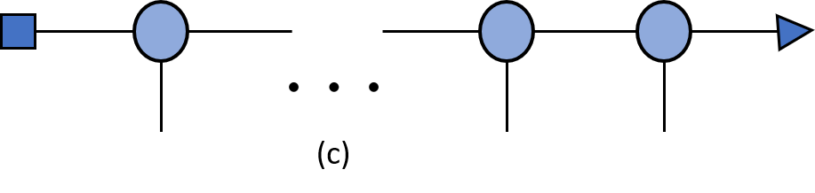
To represent a HMM we can use a special type of tensor network, called matrix product states Yang et al. 2018. Transitions between states in the HMM are described by the transition matrix ; this is a rank tensor, and is thus represented by a node with three legs as shown in Fig. S1(b). The stationary distribution of the HMM states is represented by the square, and the triangle represents , a column vector filled with s.
The probability of a particular sequence being generated by a HMM is given by
| (S1) |
This can be represented by a tensor network, as shown in Fig. S1(c). The nomenclature ‘matrix product state’ becomes clear: the sequence tensor is obtained by multiplying by a matrix at each step.
A HMM, and its tensor network representation, decompose the large tensor into products of small tensors . As a result, HMMs exponentially reduce the memory requirement of representing a stochastic process to from where is the length of the sequence, is the number of states of the HMM and is the size of output alphabet.
Supplementary Information B B: Proof of Theorem 2, Lemma 1, and Corollary 1
Here, we present our efficient method of computing the co-emission divergence rate (CDR), in the process proving Theorem 2 and Lemma 1. Every stationary stochastic process has a HMM representation Shalizi and Crutchfield 2001; we consider two stationary stochastic processes and with HMMs and , where and are the corresponding hidden states. The corresponding pictorial representations are shown in Fig. S2(a).


The co-emission probability is
| (S2) |
obtained by contracting the output indices over tensors and , as shown in the Fig. S2(b). The tensor structure in the dashed square, which repeatedly appears in the network, has four legs, i.e., is a rank tensor. Combining the left two legs together as a row index, and the right two legs as a column index, this becomes a matrix – the transfer matrix:
| (S3) |
The leftmost and rightmost tensors represent the left and right boundaries, respectively. The left boundary is a row vector with elements . The right boundary is a column vector filled with s, such that the hidden states at the last step are equally weighted, i.e., .
If is diagonalisable, it has an eigenvalue decomposition
| (S4) |
where are eigenvalues of , sorted in order of decreasing magnitude, and and are the associated right- and left-eigenvectors. Consequently, we have
| (S5) |
As is constructed from probabilities, it is non-negative. Its left- and right-leading eigenvectors are then non-negative according to the Perron-Frobenius theorem Perron 1907; Frobenius 1912. Thus, the left- and right-boundary vectors have non-zero overlap with the associated leading left- and right-eigenvectors of the matrix , and therefore the co-emission probability has the following scaling
| (S6) |
where and is positive. This scaling holds even if is not diagonalisable; this can be proved using the Jordan form of the matrix.
Using the same argument, we also have
| (S7) |
where is the leading eigenvalue of the transfer matrix and is the leading eigenvalue of the transfer matrix . Then, we have
| (S8) |
where . Thus, the distance has the desired scaling, proving Lemma 1, and in turn Theorem 2. Taking leads to
| (S9) |
and analogously,
| (S10) | ||||
| (S11) |
Therefore,
| (S12) |
This proves Corollary 1.
Supplementary Information C C: Pedagogical example of calculating the CDR

As a pedagogical example of how our efficient method for computing the CDR works, we study the distinguishability between two versions of the perturbed coin process Gu et al. 2012 (representable by the HMM in Fig. S3) with different parameters. This is a Markov process, as output indicates the hidden state is and output indicates the hidden state . Consider two perturbed coin processes and with parameters and respectively. Then the transfer matrices are
| (S13) |
Evaluating the leading eigenvalues of these matrices, we obtain
| (S14) |
Therefore, the CDR is
| (S15) |
Clearly, iff the two processes are identical, i.e., .
Supplementary Information D D: Fidelity divergence rate
Here, we present another member of the divergence rate family that also satisfies the desired properties of a process distinguishability measure. This divergence rate is called fidelity divergence rate (FDR), as the associated distance is the Bures/Hellinger distance , which is expressed in terms of the fidelity . Then , and the FDR is
| (S16) |
Similar to the CDR, we will demonstrate that exhibits the required scaling for the FDR to satisfy our requirements, and provide an efficient method for its evaluation given deterministic HMM representations of the processes. A deterministic (or unifilar) HMM is one for which the current hidden state can always be deduced with certainty given the previous state and output. This means that each state only has at most one outgoing edge for each symbol. Every stationary stochastic process has a deterministic HMM representation Shalizi and Crutchfield 2001.
Theorem 3.
The FDR satisfies all the proposed requirements for a measure of process distinguishability.
Consider two stationary stochastic processes, and , with deterministic HMM representations and , respectively, and associated transfer matrix .
Lemma 2.
scales as
The fidelity , conditioned on starting in hidden states has a pictorial representation as shown in Fig. S4(a). The left boundary represents the and standard basis vectors and in the corresponding space, while the right boundary, denoted by , is the column vector filled with s, as shown in Fig S4(b).


The tensor structure in the dashed square is the transfer matrix , which acts repeatedly on the left boundary . Similar to the proof for the co-emission, if is diagonalisable we have the eigenvalue decomposition
| (S17) |
where are the eigenvalues of sorted in order of decreasing magnitude, and and are the associated right- and left-eigenvectors. Consequently,
| (S18) |
where is the overlap between the left vector and the leading eigenvector of . Because is non-negative matrix, its left- and right-leading eigenvectors are non-negative according to the Perron-Frobenius theorem Perron 1907; Frobenius 1912. Since spans the whole space, there always exists a vector such that it has non-zero overlap with leading left eigenvector of transfer operator , i.e., . As with the co-emission, the above scaling still holds when is not diagonalisable, as can be shown using the Jordan form. Thus, we see that the fidelity decays exponentially with the length of the sequence, and thus exhibits the required scaling, proving Lemma 2 and Theorem 3.
Corollary 2.
Given deterministic HMM representations and of processes and , the FDR is given by
| (S19) |
where is the leading eigenvalue of operator .
For all boundary vectors , we have
| (S20) |
where The above quantity is the fidelity conditional on certain past . We now bound the non-conditioned fidelity in the following.
| (S21) |
The inequality implies
| (S22) |
Therefore, we have
| (S23) |
On the other hand, using inequality , we have
| (S24) |
Similarly, we also obtain
Thus, the proof is completed.
The fidelity divergence rate can thus be obtained by evaluating the leading eigenvalue of the transfer matrix . The computational complexity of this method depends only polynomially on the number of hidden states in the deterministic HMM representations of each process, and thus can be efficiently computed.
Finally, we provide upper and lower bounds for the FDR that can be calculated even when we do not have deterministic representations of the processes, from their statistics alone.
Theorem 4.
Suppose two stochastic processes have finite Markov order and the larger one is . Then the fidelity divergence rate has the following upper and lower bounds
| (S25) |
First, having Markov order implies that
| (S26) |
From this, we find that
| (S27) |
Thus, we have
| (S28) |
Substituting the above into the definition of FDR leads to
| (S29) |
The lower bound can similarly be obtained by replacing maximisations with minimisations and reversing the directions of the inequalities.