Actuation response model from sparse data for wall turbulence drag reduction
Abstract
We compute, model, and predict drag reduction of an actuated turbulent boundary layer at a momentum thickness based Reynolds number of . The actuation is performed using spanwise traveling transversal surface waves parameterized by wavelength, amplitude, and period. The drag reduction for the set of actuation parameters is modeled using 71 large-eddy simulations (LES). This drag model allows to extrapolate outside the actuation domain for larger wavelengths and amplitudes. The modeling novelty is based on combining support vector regression for interpolation, a parameterized ridgeline leading out of the data domain, scaling from Tomiyama and Fukagata 2013, and a discovered self-similar structure of the actuation effect. The model yields high prediction accuracy outside the training data range.
1 Introduction
The skin friction associated with a turbulent boundary layer constitutes about of the total drag of an airplane. Owing to its importance, passive or active skin-friction reduction means have widely been investigated (Fan and Dong 2016). Promising strategies include riblets (Walsh and Lindemann 1984), compliant surfaces (Luhar et al. 2016), spanwise wall oscillations and similar variations (Jung et al. 1992; Quadrio et al. 2009), and spanwise traveling waves of spanwise forcing (Du and Karniadakis 2000) or wall-normal deflection (Klumpp et al. 2011; Albers et al. 2019b; Albers et al. 2019a). To determine the optimal actuation settings, the parameter space is typically scanned by performing a large number of numerical simulations, which is very costly and sometimes untractable, e.g., for high Reynolds number or large actuation wavelength. This reliance on numerical simulations is partially due to the fact that experiments for many of these actuation concepts are either currently unrealizable or are limited by design to a small actuation range. In this study, a methodology is developed to model sparse flow response data to spanwise traveling surface waves using a machine learning regression algorithm for interpolation and a ridgeline modeling for extrapolation and optimization, which reduces the necessity for a large parametric study. Investigations on the boundary layer response sensitivities show a self-similar response behavior starting at a certain wavelength.
Actuation employing a spanwise pressure gradient has been shown to attenuate the boundary layer low-speed streaks and reduce turbulence production. This principle was first put into practice by a spanwise wall oscillation for turbulent channel flows (Jung et al. 1992; Touber and Leschziner 2012) and for turbulent boundary layers (Lardeau and Leschziner 2013). The actuation generates a thin spanwise Stokes layer and reduces the wall-shear stress. A more efficient variant of the spanwise actuation is the streamwise traveling wave of spanwise forcing (Quadrio et al. 2009), where a maximum drag reduction of can be achieved for turbulent channel flows. Using the same actuation technique Gatti and Quadrio 2016 performed a comprehensive study of 4020 direct numerical simulations of a channel flow with varying wavenumber, amplitude, frequency, and Reynolds number. Such a large parameter study using high-fidelity simulations is unusual and computationally very expensive. The results showed that, for channel flows, the drag reduction at higher Reynolds numbers can be estimated using the vertical shift of the logarithmic velocity profile.
Another actuation variant employs the transversal traveling wave. A first implementation was conducted for a channel flow by Du and Karniadakis 2000, where the wave effect was generated with a Lorentz force. To enable real-life applications, more recent studies proposed a similar traveling wave effect by means of surface deformation. This approach has been experimentally tested for a turbulent boundary layer by Li et al. 2018, where the surface was deflected using electromagnetic actuators. They achieved a drag reduction of . Spanwise traveling transversal surface waves have also been numerically simulated for a turbulent boundary layer over a flat plate (Albers et al. 2019a), with a maximum drag reduction of , and over a wing section (Albers et al. 2019b), where the pressure varies in the streamwise direction. For the wing flow, the total drag was reduced by and a slight lift increase was also achieved.
Drag reduction optimization in a rich actuation space constitutes a challenge. In experimental setups, many degrees of freedom are fixed by design, whereas high-fidelity high Reynolds number simulations are able to explore a rich spectrum of actuation settings. However, high-fidelity numerical computations are costly and thus limited to a small number of control laws. Surrogate models are computationally cheap models that approximate the behavior of complex systems, based on a limited number of data. Surrogate models are typically used for optimization (Forrester and Keane 2009; Yondo et al. 2018) and for visualization and design space analysis (Holden 2004). There exists many approaches and algorithms. The Response Surface Methodology (RSM) is one of the earliest approaches (Box and Wilson 1951). The models from RSM are often polynomials up to second order (Sevant et al. 2000; Madsen and Shyy 2000; Ahn et al. 2001; Karami et al. 2016), which can not represent highly non-linear or multi-modal design landscapes. Radial basis functions (RBF) is an interpolation technique based on a weighted sum of radial basis functions (Broomhead and Lowe 1988). Various types of basis functions can be used to accommodate the response surface complexity (Forrester and Keane 2009). RBF surrogate models have successfully been used to optimize groundwater remediation design (Akhtar and Shoemaker 2016). Another widely used technique is kriging, which is a kernel-based probabilistic approach (Matheron 1963). Kriging models can yield high predictive power (Forrester and Keane 2009) and have been used, for instance, to optimize a airfoil geometry (Jeong et al. 2005).
Other computationally more expensive algorithms include support vector regression (SVR) (Drucker et al. 1997), and artificial neural network (ANN), first developed by McCulloch and Pitts 1943. SVR is a kernel-based regression technique, which tolerates predictions errors within an user-defined interval. More details about SVR are given in section 3.2. SVR has been shown to outperform RSM, kriging, and RBF for a test bed of 26 complex engineering functions (Clarke et al. 2005), and has successfully been used to optimize railway wind barriers (Xiang et al. 2017). ANNs are non-linear regression models inspired by biological neural networks. They have been used to accurately predict the drag reduction in oil pipelines (Zabihi et al. 2019).
A common shortcoming of data-driven surrogate models is their rapidly diminishing accuracy outside the training parameter range. This limitation means strong disadvantages for the investigated boundary layer application. Initial analyses have shown a higher drag reduction trend leading beyond the training parameter space, where simulations become increasingly less affordable.
In this study, we present a new modeling methodology capable of extrapolating drag reduction beyond the parameter range. The starting point is a sparse set of 71 large-eddy simulations (LES) of a turbulent boundary layer actuated by spanwise traveling transversal waves. Our approach consists of two steps: First, a surrogate model is built using SVR to interpolate the drag reduction in the training parameter space. Then, extrapolation is enabled through the identification of a ridgeline in the drag reduction response. The model is used to analyze the actuation sensitivities and to infer higher drag reduction and the corresponding actuation settings.
The paper is structured as follows. The numerical method of the high-fidelity simulations and the computational setup of the flat plate undergoing transversal spanwise traveling waves are defined in section 2. The modeling approach is described in section 3 for a simple problem, before being applied to the actuated boundary layer data in section 4. Finally, conclusions are presented in section 5.
2 Numerical setup
In this section, the open-loop actuation study of wall turbulence drag reduction is recapitulated. In particular, the investigated actuation parameters are enumerated. Section 2.1 describes the configuration, while section 2.2 details the employed large-eddy simulation (LES) solver.
2.1 Configuration
The fluid flow is described in a Cartesian frame of reference where the streamwise, wall-normal, and spanwise coordinates are denoted by and the velocity components by . The Mach number is set to such that nearly incompressible flow is considered. An illustration of the rectangular physical domain is shown in figure 1. A momentum thickness of at is achieved such that the momentum thickness based Reynolds number is at . The domain length and height in the streamwise and wall-normal direction are and . In the spanwise direction, different domain widths are used to simulate different actuation wavelengths.
At the domain inlet, a synthetic turbulence generation method is applied to generate a natural turbulent boundary layer flow after a transition length of 2-4 boundary layer thicknesses (Roidl et al. 2013). Characteristic boundary conditions are used at the domain exit and a no-slip wall boundary condition is enforced at the lower domain boundary for the unactuated and actuated wall. The wall actuation is prescribed by the space- and time-dependent function
| (1) |
in the interval . The quantities , , and denote the wavelength, period, and amplitude in inner coordinates, i.e., the parameters are scaled by the viscosity and the friction velocity of the unactuated reference case . In the area just upstream and downstream of the wave actuation region, a spatial transition is used from a flat plate to an actuated plate and vice versa Albers et al. 2019a. In total, 71 actuation configurations with wavelength , period , and amplitude are simulated. Two additional validation simulations are performed for , , and and for , , and . All operating conditions and the corresponding drag reductions are listed in appendix B. The current setup is identical to that in Ishar et al. 2019. However, a considerably larger parameter set is computed in this study, containing also larger wavelengths.
The physical domain is discretized by a structured block-type mesh with a resolution of in the streamwise and in the spanwise direction. In the wall-normal direction, a resolution of at the wall is used with gradual coarsening away from the wall. Depending on the domain width, the meshes consist of to million cells.
The simulation procedure is as follows. First, the reference simulations for all domain widths are run for convective time units. Then, the actuated simulations are initialized by the solution from the unactuated reference case and the temporal transition from the flat plate to the actuated wall is initiated. When a converged state of the friction drag is obtained, statistics are collected for convective times.
The drag coefficient is computed by integrating the wall-shear stress over the streamwise interval and over the entire domain spanwise width, i.e., the colored surface in figure 1
The quantities , denote the unit normal vector of the surface and the unit vector in the -direction, the reference surface is . The drag reduction is defined as
where the superscripts and refer to the unactuated reference and actuated cases.
2.2 Numerical method
The actuated flat plate turbulent boundary layer flow is governed by the unsteady compressible Navier-Stokes equations in the arbitrary Lagrangian-Eulerian formulation for time-dependent domains. A second-order accurate finite-volume approximation of the governing equations is used in which the convective fluxes are computed by the advection upstream splitting method (AUSM) and time integration is performed via a 5-stage Runge-Kutta scheme. The smallest dissipative scales are implicitly modeled through the numerical dissipation of the AUSM scheme. This monotonically integrated large-eddy simulation approach (Boris et al. 1992) is capable of accurately capturing all physics of the resolved scales (Meinke et al. 2002). Further details on the numerical method can be found in Albers et al. 2019b and Ishar et al. 2019.
3 Methodology
In this section, we propose a data-driven response surface methodology for interpolation and extrapolation. The methodology is developed to handle the observed relative drag reduction sensitivities . We note that is positive for reduced drag. Initial analyses indicate that, for the spanwise traveling wave, in every plane, the drag reduction features a single global maximum with respect to the actuation period and amplitude of the current spanwise traveling wave type. The curve of connecting all these -dependent maxima is the ridgeline, denoted by the subscript . These optimal amplitude and period increase with beyond the currently simulated parameter range. Such response behavior is challenging for optimization and requires specially-developed tools.
Section 3.1 introduces an analytical example which features similar topology to the drag reduction response distribution. The machine learning algorithm used to interpolate the response within the parameter range is detailed in section 3.2. In section 3.3, a novel data-driven modeling approach is proposed and exemplified for the analytical example.
3.1 Analytical response surface
To sharpen our data-driven tools, we start with an analytic response function which behaves qualitatively similar to the drag reduction problem. From the parameter vector , mimics the wavelength, the period, and the amplitude. The analytical example
| (2) |
is investigated in the domain
| (3) |
The function factors into one monotonously increasing term and one -independent monomodal term with a single maximum in . At a given , assumes the maximum on the ridgeline , . The ridgeline marks the maxima of and for constant . The global maximum in the domain is at the boundary .
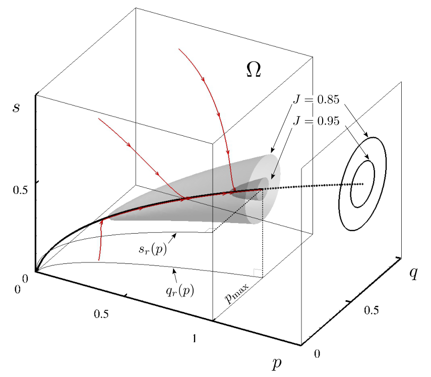
These trends are observed in figure 2, which illustrates the analytical response surface as iso-surfaces, the ridgeline (black), and the lines of steepest ascent (red). The lines of steepest ascent provide a direct indication to the response sensitivities and point in the direction of the global optima. The lines of steepest ascent are simply streamlines of the gradient field seeded from various points.
Evidently, larger values are obtained outside the domain on the ridgeline. Following this curve is a good extrapolation strategy for testing new and better parameters. The extrapolation to suboptimal parameters outside the domain is facilitated by the self-similar structure of this particular response function. The response can be parameterized by a -dependent function multiplying a properly scaled -dependent function
| (4) |
where
| (5a) | |||||
| (5b) | |||||
Thus, knowing in a plane allows to extrapolate all response functions for via equation (4).
3.2 Support vector regression
In this study, the analytical response formula from sparse data point is obtained by support vector regression (SVR) (Cortes and Vapnik 1995; Drucker et al. 1997). SVR belongs to the family of supervised-learning algorithms that trains from observations to find a mapping between features or inputs , and the corresponding response , . In the application presented in section 4, the features are the wavelength , period , and amplitude and the output is the relative drag reduction .
Following good practices of machine learning (Burkov 2019), the inputs for the response formula are centered features which are normalized to unit variance. This normalization gives every feature a similar weight in interpolation. In this study, the normalization is particularly important as the ranges of investigated wavelengths and periods differ by more than one order of magnitude.
SVR yields a regression model smoothly interpolating from data points , , employing a Gaussian Kernel and optimized weights :
| (6) |
Here, is a constant to which converges far away from the data points, denotes the weight vector, and comprises the Gaussian Kernel functions.
Calibrating the response model (6) for , leads to linear equations for weights . Under generic conditions, such a linear system can be solved and the formula will exactly reproduce the input data. Yet, this vanishing in-sample error may come at the price of overfitting. Noise may be incorporated as data feature, thus leading to an unphysical model complexity. The over-fitted model may amplify noise outside the training data, implying a large generalization error or, equivalently, a large out-of-sample error.
To account for noise and new data points, an error of is tolerated, i.e., a prediction is accepted. The generalization error of the formula is reduced by avoiding unnecessary complexity, e.g., by replacing two Kernels of very close collocation points with a single one. Complexity is characterized and penalized by the vector norm . This leads to the regularized optimization problem
| (7) | ||||
However, weights which satisfy the -constraint at all points might not exist, particularly for the validation data. This constraint is relaxed by introducing so-called slack variables in case and if . The slack variables extend the permissible -interval for to . Now, the relaxed regularized optimization problem becomes
| (8) | ||||
The tradeoff between model complexity and errors beyond the limit is controlled by the penalty parameter . The extreme choice leads to unpenalized, arbitrarily large slack variables and minimal complexity since the minimization solely focuses on . In other words, is a constant function. For sufficiently large , the accuracy of the response model is optimized tolerating maximum complexity. The value of is set to the data noise level, if available. Note that too large a value will decrease the prediction accuracy.
The interpolation is performed with the radial basis function
| (9) |
The reader can refer to (Forrester and Keane 2009) for more details about the SVR formulation and the solution of the constrained optimization problem (8).
3.3 Data-driven response surface
The analytical example preludes our data-driven approach for the actuated turbulent boundary layer. The approach consists of the following steps:
- Step 1
-
We consider computed response function values for parameter points , , covering well the parameter range of interest . Each parameter may need to be centered and scaled to unit variance for the regression problem.
- Step 2
-
Interpolate all function values in the domain with an accurate and smooth machine learning regression.
- Step 3
-
Apply a gradient search technique for several initial conditions. If the corresponding steepest ascent curves converge to a point inside the domain, the purpose of a response surface model is served.
- Step 4
-
Identify the ridgeline coordinates () and response leading out of the domain , and model them using simple functions. This simple model can now be used to extrapolate the ridgeline outside towards the global response optimum. Note the choice of the parametrizing ridgeline parameter (here: ) is problem-dependent.
- Step 5
-
In some cases, like in the example (2), the response function exhibits self-similar behavior, and can be expressed as a -dependent function multiplying a scaled -dependent function as:
where is the ridgeline response, and is a shape function with the maximum . In this case, the shape function and extrapolated ridgeline can be used to predict the response to parameter inputs away from the ridgeline.
Note that the parameters , , and used in this analytical example correspond to the wavelength , period , and amplitude for the boundary layer application.
4 Results
The previous section discussed the modeling methodology of response functions, which assumes the optimal value at the boundary of the explored parameter space. This section applies the approach to drag reduction for an actuated boundary layer with spanwise traveling surface waves. We follow the steps outlined in section 3.

The process begins with the interpolation of the sparse parameter space using support vector regression (SVR). As presented in section 2, the investigated parameter space spanned by , , and is large, and a dense coverage is beyond the reach of feasibility. The SVR algorithm is chosen for its prediction accuracy and its smooth response distribution (see appendix A for details). The algorithm is trained on a subset of of the dataset, whilst the remaining is used for testing the prediction performance. This separation of training and testing data reduces the risk of overfitting. The algorithm hyperparameters are tuned using 3-fold cross-validation. In this study, the SVR model yields , the definition of which is given in appendix A. This value indicates excellent prediction accuracy. Using the SVR model, we interpolate the parameter space with drag coefficient predictions.
With the parameter space densely populated, it is now possible to compute and to visualize the streamlines of the gradient field and the ridgeline. It is shown in figure 3 (d) that the streamlines (red) and the ridgeline (solid black line) terminate at the domain boundary in the - plane at the exit point (, , and ). This indicates that the optimal drag reduction lies outside the current range. Along the ridgeline, the relative drag reduction increases from at to at the ridgeline exit point .
Figure 4 shows the projection of the ridgeline onto the – and – planes. Starting at , asymptotes rapidly toward 44. In other words, the optimum wave period remains constant at , even with increasing wavelength and amplitude. Similarly, shows an asymptotic behavior with higher , albeit at a slower rate.

This asymptotic behavior of the ridgeline starting at is easily modeled as
| (10) |
The fitted curves are presented in figure 4 by dotted lines and show good agreement with the reference lines over the common range ().
Having established the and sole dependence on along the ridgeline, we turn our attention to drag reduction. Similarly to and , also shows the sole dependence on or equivalently on and . This is best expressed using a scaling proposed by Tomiyama and Fukagata 2013, defined as , which is the product of the velocity amplitude of the actuation and the thickness of the Stokes layer along the ridge. Note that this scaling is originally defined for the skin-friction coefficient, but for the considered cases, the amount of added wetted surface is negligible and the scaling holds (Albers et al. 2019a). The evolution of towards a linear behavior is illustrated in figure 5. As the figure shows, the drag reduction along the ridge starts exhibiting linearity around corresponding approximately to . It is worth to note that this almost perfect linear Tomiyama and Fukagata scaling only holds along the ridgeline. Away from the ridgeline, the scaling shows scatter.

It is now straightforward to model the relative drag reduction in the linear range, i.e., , as
| (11) |
This linear fit is shown with a dotted line in figure 5 as function of the Tomiyama and Fukagata scaling, and in figure 4 as a function of . Note that we assume that the linear behavior continues for a finite range beyond .
Based on the optimal drag reduction behavior being only dependent on , which is consistent with a self-similar behavior, we assume a response of the form
| (12) |
where is the constant-linear model from substituting equation 10 into equation 11, and and are properly scaled actuation parameters. The natural scaling choice is the maximum relative drag reduction along the ridgeline, which yields
| (13) |
Hence, self-similarity is validated when becomes independent of . This is confirmed in figures 3 (a), (b), and (c), where the distributions collapse starting at .
Note that the preceding analysis did not only examine the sensitivities of the flow response and its self-similar behavior, but also yielded a simple powerful model of the relative drag reductions.
This self-similar drag reduction model for proceeds as follows:
- •
For given actuation setting , and , compute and from equation 10.
- •
Determine the drag reduction along the ridgeline using equation 11.
- •
Read from the distributions in figure 3.
- •
Deduce the relative drag reduction from .
In the interpolation regime, and for , this simple model has a coefficient of determination of , which is very close to that of the SVR model. In the extrapolation regime, the model is validated with two points at , which is well beyond the training range. The first validation point B is situated on the ridgeline (cf. figure 3), whereas the second point is off the ridgeline at coordinates , , and . For these two operating conditions, the relative drag reductions predicted by the model are and , which compare favorably with those of the reference LES data of and . These predictions yield relative errors of and for and , respectively.
The prediction accuracy for the extrapolation at , i.e., beyond the maximal investigated values is impressive. Yet, the model (12) should not be assumed to hold at much larger wavelengths (). In this limit, the actuation approaches that of a flat plate moving up and down without height variations in the spanwise direction. In this scenario, the boundary layer remains unchanged and no drag reductions can be expected.
5 Conclusions
We target improved drag reduction of an actuated turbulent boundary layer with spanwise traveling surface waves at . 71 large-eddy simulations are used to determine a machine learned model to predict drag reduction as a function of the actuation parameters: amplitude, period, and spanwise wavelength. The first enabler for this formula is the support vector regression (SVR) for smooth interpolation. For this dataset, SVR is found to be distinctly superior to many other common regression solvers. The second enabler is a ridgeline pointing outside the computed domain indicating further drag reduction potential at unexplored higher wavelengths. This ridgeline is then modeled and used for extrapolation. The results indicate a potential around drag reduction with increasing wavelength, which is denoted as point B in figure 3. This result is confirmed by an additional LES. The corresponding period seems to asymptote against 44 plus units while the amplitude slowly increases with wavenumber. The ridgeline parameters are consistent with the Tomiyama and Fukagata scaling. More precisely, at wavelengths above 1000 plus units within the analyzed range, the drag reduction linearly increases with the Tomiyama and Fukagata parameter on the ridgeline.
Surprisingly, the drag reduction formula exhibits a self-similar behavior starting at . As such, drag reduction can be expressed as the product of a factor depending only on the wavelength and a shape factor depending on amplitude and period normalized with their ridgeline values. The ridgeline parameters and the drag reduction values in a plane with constant wavelength allow to extrapolate drag values for amplitudes and periods for wavelengths above 1000 plus units. The self-similar drag reduction formula beautifully parameterizes all investigated simulations and allow to predict further performance potential at unexplored larger wavelengths.
The proposed machine learning method for the drag reduction formula can easily be applied to other performance parametrics from sparse data. The strategy is (1) to interpolate the sparse parameter space using an accurate machine learning algorithm; (2) to compute several steepest ascent lines and ridgelines; (3) to search for the global optimum inside the domain; (4) if the steepest ascent lines terminate at the boundary to extrapolate the ridgeline out of the domain; (5) to test for self-similarity based on this ridgeline. Self-similarity opens the possibility to extrapolate the performance away from the ridgeline.
The drag reduction formula may guide future simulations in search of larger drag reduction. In addition, the observed self-similarity guides and constrains future physics-based models. The authors actively explore these avenues.
Acknowledgements
The research was funded by the Deutsche Forschungsgemeinschaft (DFG) in the framework of the research projects SE 2504/2-1, SCHR 309/52 and SCHR 309/68. The authors gratefully acknowledge the Gauss Centre for Supercomputing e.V. (www.gauss-centre.eu) for funding this project by providing computing time on the GCS Supercomputers Hazelhen at HLRS Stuttgart and JURECA at Jülich Supercomputing Centre (JSC). BRN acknowledges support from the French National Research Agency (ANR) under grant ANR-17-ASTR-0022 (FlowCon).
Appendix A Machine learning regression model
Drag reduction modeling as a function of the actuation parameters for the actuated boundary layer is a challenging problem. The complexity of the response topology led to the utilization of machine learning (ML) approaches. For this application, ML is used to model the drag reduction under varying actuation conditions (, and ). ML algorithms are evaluated based on their prediction accuracy, given by the coefficient of determination , defined as
| (14) |
where are the reference computed data points, are the predicted ones, is the mean of , and is the number of samples in the test set. A value of denotes perfect prediction score. Besides accuracy, the model smoothness is the second criterion for the model selection. The ML algorithm smoothness was quantified with the total variation (TV) defined as
| (15) |
where , , and are the number of discretized points in the , , and directions. A smooth response is indicated by a lower TV value. Three machine learning algorithms were benchmarked: the -nearest neighbors (kNN), random forest (RF), and support vector regression (SVR). The hyperparameters of each algorithm were optimized using cross-validation, yielding 5 neighbors for kNN and 300 trees for RF. Radial basis functions are used for SVR. The and TV values for the three algorithms are summarized in table 1.
| Algorithm | ||
|---|---|---|
| kNN | 0.76 | |
| RF | 0.97 | |
| SVR | 0.93 |
Based on the results, SVR offers the best compromise between smoothness and accuracy; it is smoother than RF and more accurate than kNN. Therefore, it is selected for this study.
Appendix B Operating conditions of the LES simulations
| 1 | 1000 | 500 | 20 | 30 | 0 | 4 | 3.5 |
| 2 | 1000 | 500 | 30 | 22 | 9 | 10 | 1.9 |
| 3 | 1000 | 500 | 40 | 21 | 8 | 9 | 1.7 |
| 4 | 1000 | 500 | 40 | 30 | 8 | 11 | 3.5 |
| 5 | 1000 | 500 | 60 | 30 | 5 | 8 | 3.5 |
| 6 | 1000 | 500 | 70 | 36 | 3 | 8 | 4.9 |
| 7 | 1000 | 500 | 70 | 64 | -10 | 4 | 14.6 |
| 8 | 1000 | 500 | 100 | 48 | -3 | 5 | 8.6 |
| 9 | 1000 | 1000 | 20 | 10 | 5 | 5 | 0.1 |
| 10 | 1000 | 1000 | 20 | 30 | 13 | 13 | 0.9 |
| 11 | 1000 | 1000 | 20 | 50 | 0 | 3 | 2.4 |
| 12 | 1000 | 1000 | 40 | 10 | 3 | 3 | 0.1 |
| 13 | 1000 | 1000 | 40 | 20 | 7 | 8 | 0.4 |
| 14 | 1000 | 1000 | 40 | 30 | 12 | 13 | 0.9 |
| 15 | 1000 | 1000 | 40 | 40 | 15 | 16 | 1.6 |
| 16 | 1000 | 1000 | 40 | 50 | 15 | 17 | 2.4 |
| 17 | 1000 | 1000 | 40 | 60 | 13 | 16 | 3.5 |
| 18 | 1000 | 1000 | 80 | 10 | 1 | 1 | 0.1 |
| 19 | 1000 | 1000 | 80 | 20 | 3 | 4 | 0.4 |
| 20 | 1000 | 1000 | 80 | 30 | 6 | 6 | 0.9 |
| 21 | 1000 | 1000 | 80 | 40 | 9 | 10 | 1.6 |
| 22 | 1000 | 1000 | 80 | 50 | 9 | 11 | 2.4 |
| 23 | 1000 | 1000 | 80 | 60 | 9 | 12 | 3.5 |
| 24 | 1000 | 1000 | 120 | 10 | 1 | 1 | 0.1 |
| 25 | 1000 | 1000 | 120 | 20 | 0 | 1 | 0.4 |
| 26 | 1000 | 1000 | 120 | 30 | 3 | 4 | 0.9 |
| 27 | 1000 | 1000 | 120 | 40 | 3 | 5 | 1.6 |
| 28 | 1000 | 1000 | 120 | 50 | 2 | 5 | 2.4 |
| 29 | 1000 | 1000 | 120 | 60 | 2 | 6 | 3.5 |
| 30 | 1200 | 600 | 30 | 44 | 2 | 7 | 5.1 |
| 31 | 1200 | 600 | 40 | 59 | -4 | 5 | 8.9 |
| 32 | 1200 | 600 | 50 | 36 | 9 | 12 | 3.5 |
| 33 | 1200 | 600 | 60 | 21 | 5 | 6 | 1.2 |
| 34 | 1200 | 600 | 70 | 29 | 6 | 8 | 2.3 |
| 35 | 1200 | 600 | 80 | 66 | -5 | 6 | 11.0 |
| 36 | 1200 | 600 | 90 | 51 | -1 | 6 | 6.8 |
| 37 | 1200 | 600 | 100 | 14 | 2 | 2 | 0.5 |
| 38 | 1600 | 1600 | 20 | 22 | 11 | 11 | 0.2 |
| 39 | 1600 | 1600 | 40 | 34 | 14 | 14 | 0.4 |
| 40 | 1600 | 1600 | 40 | 48 | 19 | 19 | 0.9 |
| 41 | 1600 | 1600 | 50 | 60 | 19 | 20 | 1.4 |
| 42 | 1600 | 1600 | 50 | 73 | 21 | 22 | 2.0 |
| 43 | 1600 | 1600 | 60 | 27 | 8 | 8 | 0.3 |
| 44 | 1600 | 1600 | 70 | 71 | 17 | 19 | 1.9 |
| 45 | 1600 | 1600 | 80 | 17 | 2 | 2 | 0.1 |
| 46 | 1600 | 1600 | 90 | 65 | 13 | 14 | 1.6 |
| 47 | 1600 | 1600 | 100 | 40 | 8 | 8 | 0.6 |
| 48 | 1800 | 900 | 30 | 49 | 10 | 12 | 2.9 |
| 49 | 1800 | 900 | 40 | 63 | 7 | 12 | 4.7 |
| 50 | 1800 | 900 | 50 | 22 | 7 | 7 | 0.6 |
| 51 | 1800 | 900 | 50 | 44 | 12 | 14 | 2.3 |
| 52 | 1800 | 900 | 70 | 28 | 7 | 8 | 0.9 |
| 53 | 1800 | 900 | 80 | 17 | 3 | 4 | 0.4 |
| 54 | 1800 | 900 | 80 | 60 | 6 | 9 | 4.3 |
| 55 | 1800 | 900 | 90 | 39 | 6 | 7 | 1.8 |
| 56 | 1800 | 1800 | 30 | 14 | 5 | 5 | 0.1 |
| 57 | 1800 | 1800 | 40 | 51 | 19 | 20 | 0.8 |
| 58 | 1800 | 1800 | 40 | 70 | 22 | 23 | 1.5 |
| 59 | 1800 | 1800 | 50 | 59 | 20 | 21 | 1.1 |
| 60 | 1800 | 1800 | 60 | 44 | 15 | 15 | 0.6 |
| 61 | 1800 | 1800 | 60 | 75 | 21 | 22 | 1.7 |
| 62 | 1800 | 1800 | 70 | 29 | 7 | 7 | 0.3 |
| 63 | 1800 | 1800 | 80 | 36 | 9 | 9 | 0.4 |
| 64 | 1800 | 1800 | 90 | 66 | 13 | 14 | 1.3 |
| 65 | 1800 | 1800 | 100 | 21 | 3 | 3 | 0.1 |
| 66 | 3000 | 3000 | 40 | 51 | 21 | 21 | 0.3 |
| 67 | 3000 | 3000 | 50 | 78 | 26 | 26 | 0.7 |
| 68 | 3000 | 3000 | 60 | 26 | 7 | 7 | 0.1 |
| 69 | 3000 | 3000 | 70 | 64 | 19 | 19 | 0.4 |
| 70 | 3000 | 3000 | 80 | 11 | 1 | 1 | 0.0 |
| 71 | 3000 | 3000 | 90 | 66 | 16 | 16 | 0.5 |
| 5000 | 5000 | 44 | 99 | 31 | 31 | 0.0 | |
| 5000 | 5000 | 44 | 92 | 30 | 30 | 0.0 |
References
- Ahn et al. [2001] J. Ahn, H.-J. Kim, and O.H. Lee, D.-H. Rho. Response surface method for airfoil design in transonic flow. Journal of Aircraft, 38(2):231–238, 2001.
- Akhtar and Shoemaker [2016] T. Akhtar and C. A. Shoemaker. Multi objective optimization of computationally expensive multi-modal functions with RBF surrogates and multi-rule selection. Journal of Global Optimization, 64(1):17–32, January 2016.
- Albers et al. [2019a] M. Albers, P. S. Meysonnat, D. Fernex, R. Semaan, B. R. Noack, and W. Schröder. Drag reduction and energy saving by spanwise traveling transversal surface waves for flat plate flow. arXiv preprint arXiv:1908.09565, 2019a.
- Albers et al. [2019b] M. Albers, P. S. Meysonnat, and W. Schröder. Actively reduced airfoil drag by transversal surface waves. Flow, Turbulence and Combustion, 102(4):865–886, Jan 2019b.
- Boris et al. [1992] J. P. Boris, F. F. Grinstein, E. S. Oran, and R. L. Kolbe. New insights into large eddy simulation. Fluid Dynamics Research, 10(4-6):199–228, 1992.
- Box and Wilson [1951] G. E. P. Box and K. B. Wilson. On the experimental attainment of optimum conditions. Journal of the Royal Statistical Society: Series B (Methodological), 13(1):1–38, 1951.
- Broomhead and Lowe [1988] D. S. Broomhead and D. Lowe. Radial basis functions, multi-variable functional interpolation and adaptive networks. Technical Report RSRE-MEMO-4148, Royal Signals and Radar Establishment Malvern (United Kingdom), March 1988.
- Burkov [2019] A. Burkov. The Hundred-Page Machine Learning Book. Andriy Burkov, 2019.
- Clarke et al. [2005] S. M. Clarke, J. H. Griebsch, and T. W. Simpson. Analysis of support vector regression for approximation of complex engineering analyses. Journal of Mechanical Design, 127(6):1077–1087, November 2005.
- Cortes and Vapnik [1995] C. Cortes and V. Vapnik. Support-vector networks. Machine Learning, 20(3):273–297, September 1995.
- Drucker et al. [1997] H. Drucker, C. J. C. Burges, L. Kaufman, A. J. Smola, and V. Vapnik. Support vector regression machines. In Advances in Neural Information Processing Systems, pages 155–161. MIT Press, 1997.
- Du and Karniadakis [2000] Y. Du and G. Karniadakis. Suppressing wall turbulence by means of a transverse traveling wave. Science, 288(5469):1230–1234, June 2000.
- Fan and Dong [2016] B. Fan and G. Dong. Principles of Turbulence Control. National Defense Industry Press with Wiley, 2016.
- Forrester and Keane [2009] A. I. J. Forrester and A. J. Keane. Recent advances in surrogate-based optimization. Progress in Aerospace Sciences, 45(1):50–79, January 2009.
- Gatti and Quadrio [2016] D. Gatti and M. Quadrio. Reynolds-number dependence of turbulent skin-friction drag reduction induced by spanwise forcing. Journal of Fluid Mechanics, 802:553–582, September 2016.
- Holden [2004] C. M. E. Holden. Visualization methodologies in aircraft design optimization. PhD thesis, University of Southampton, 2004.
- Ishar et al. [2019] R. Ishar, E. Kaiser, M. Morzyński, D. Fernex, R. Semaan, M. Albers, P. S. Meysonnat, W. Schröder, and B. R. Noack. Metric for attractor overlap. Journal of Fluid Mechanics, 874:720–755, September 2019.
- Jeong et al. [2005] S. Jeong, M. Murayama, and K. Yamamoto. Efficient optimization design method using Kriging model. Journal of Aircraft, 42(2):413–420, 2005.
- Jung et al. [1992] W. J. Jung, N. Mangiavacchi, and R. Akhavan. Suppression of turbulence in wall-bounded flows by high-frequency spanwise oscillations. Physics of Fluids A: Fluid Dynamics, 4(8):1605–1607, 1992.
- Karami et al. [2016] H. R. Karami, M. Keyhani, and D. Mowla. Experimental analysis of drag reduction in the pipelines with response surface methodology. Journal of Petroleum Science and Engineering, 138:104–112, February 2016.
- Klumpp et al. [2011] S. Klumpp, M. Meinke, and W. Schröder. Friction drag variation via spanwise transversal surface waves. Journal of Turbulence, 87(1):33–53, 2011.
- Lardeau and Leschziner [2013] S. Lardeau and M. A. Leschziner. The streamwise drag-reduction response of a boundary layer subjected to a sudden imposition of transverse oscillatory wall motion. Physics of Fluids, 25(7):075109, July 2013.
- Li et al. [2018] W. Li, D. Roggenkamp, T. Hecken, W. Jessen, M. Klaas, and W. Schröder. Parametric investigation of friction drag reduction in turbulent flow over a flexible wall undergoing spanwise transversal traveling waves. Experiments in Fluids, 59(6):105, 2018.
- Luhar et al. [2016] M. Luhar, A. S. Sharma, and B. J. McKeon. On the design of optimal compliant walls for turbulence control. Journal of Turbulence, 17(8):787–806, 2016.
- Madsen and Shyy [2000] J. I. Madsen and R. T. Shyy, W. and Haftka. Response surface techniques for diffuser shape optimization. AIAA Journal, 38(9):1512–1518, 2000.
- Matheron [1963] G. Matheron. Principles of geostatistics. Economic Geology, 58(8):1246–1266, December 1963.
- McCulloch and Pitts [1943] W. S. McCulloch and W. Pitts. A logical calculus of the ideas immanent in nervous activity. Bulletin of Mathematical Biophysics, 5(4):115–133, December 1943.
- Meinke et al. [2002] M. Meinke, W. Schröder, E. Krause, and T. Rister. A comparison of second- and sixth-order methods for large-eddy simulations. Computers and Fluids, 31(4):695–718, 2002.
- Quadrio et al. [2009] M. Quadrio, P. Ricco, and C. Viotti. Streamwise-travelling waves of spanwise wall velocity for turbulent drag reduction. Journal of Fluid Mechanics, 627:161–178, May 2009.
- Roidl et al. [2013] B. Roidl, M. Meinke, and W. Schröder. A reformulated synthetic turbulence generation method for a zonal RANS–LES method and its application to zero-pressure gradient boundary layers. International Journal of Heat Fluid Flow, 44:28–40, 2013.
- Sevant et al. [2000] N. E. Sevant, M. I. G. Bloor, and M. J. Wilson. Aerodynamic design of a flying wing using response surface methodology. Journal of Aircraft, 37(4):562–569, 2000.
- Tomiyama and Fukagata [2013] N. Tomiyama and K. Fukagata. Direct numerical simulation of drag reduction in a turbulent channel flow using spanwise traveling wave-like wall deformation. Physics of fluids, 25(10):105115, 2013.
- Touber and Leschziner [2012] E. Touber and M. A. Leschziner. Near-wall streak modification by spanwise oscillatory wall motion and drag-reduction mechanisms. Journal of Fluid Mechanics, 693:150–200, February 2012.
- Walsh and Lindemann [1984] M. J. Walsh and M. Lindemann. Optimization and application of riblets for turbulent drag reduction. In AIAA 22nd Aerospace Sciences Meeting, January 1984.
- Xiang et al. [2017] H. Xiang, Y. Li, H. Liao, and C. Li. An adaptive surrogate model based on support vector regression and its application to the optimization of railway wind barriers. Structural and Multidisciplinary Optimization, 55(2):701–713, February 2017.
- Yondo et al. [2018] R. Yondo, E. Andrés, and E. Valero. A review on design of experiments and surrogate models in aircraft real-time and many-query aerodynamic analyses. Progress in Aerospace Sciences, 96:23–61, January 2018.
- Zabihi et al. [2019] R. Zabihi, D. Mowla, and H. R. Karami. Artificial intelligence approach to predict drag reduction in crude oil pipelines. Journal of Petroleum Science and Engineering, 178:586–593, July 2019.