Non-Markovian temporal networks with auto- and cross-correlated link dynamics
Abstract
Many of the biological, social and man-made networks around us are inherently dynamic, with their links switching on and off over time. The evolution of these networks is often non-Markovian, and the dynamics of their links correlated. Hence, to accurately model these networks, predict their evolution, and understand how information and other quantities propagate over them, the inclusion of both memory and dynamical dependencies between links is key. We here introduce a general class of models of temporal networks based on discrete autoregressive processes. As a case study we concentrate on a specific model within this class, generating temporal networks with a specified underlying backbone, and with precise control over the dynamical dependencies between links and the strength and length of their memories. In this network model the presence of each link is influenced by its own past activity and the past activities of other links, as specified by a coupling matrix, which directly controls the causal relations and correlations among links. We propose a method for estimating the models parameters and how to deal with heterogeneity and time-varying patterns, showing how the model allows for a more realistic description of real world temporal networks and also to predict their evolution. We then investigate the role that memory and correlations in link dynamics have on processes occurring over a temporal network by studying the speed of a spreading process, as measured by the time it takes for diffusion to reach equilibrium. Through both numerical simulations and analytical results, we are able to separate the roles of autocorrelations and neighbourhood correlations in link dynamics, showing that the speed of diffusion is non-monotonically dependent on the memory length, and that correlations among neighbouring links can speed up the spreading process, while autocorrelations slow it down.
I Introduction
Much of the world we experience is governed by interactions. Networks provide a natural way of modelling these interactions, and as such the study of networks has been central to the understanding of both natural phenomena and man-made systems. Observably, many of the networks around us change over time, as the interactions and connections that define them come and go. Human contacts and social interactions do not last forever González et al. 2008; Starnini et al. 2013; Yoneki et al. 2009, roads between towns and cities can be closed or new ones build Murcio et al. 2015; Li et al. 2015, financial or economic agents trade each day with different counterparts Mazzarisi et al. 2020a, and even our brains undergo significant changes throughout our lives Valencia et al. 2008; Fallani et al. 2008; Millán et al. 2018; Chialvo 2010. Real-world examples of temporal networks are often found to have a set of very well defined structural and temporal features, many of which play key roles in determining the dynamics and functioning of the systems for which they form the backbone Grindrod and Higham 2010; Holme and Saramäki 2012; Masuda and Lambiotte 2016; Gauvin et al. 2014; Zanin et al. 2009; Nicosia et al. 2012; Weng et al. 2017; Peixoto and Rosvall 2017. Various models have been recently proposed to replicate such features. For instance, models of human face-to face interactions often rely on the assumption that the agents move as random walkers in a physical space and create a link whenever they are closer than a certain distance Starnini et al. 2013; Buscarino et al. 2008. Other models take a slightly more abstract approach, introducing the notion of node activity to control the presence of links Starnini and Pastor-Satorras 2014; Karsai et al. 2014; Alessandretti et al. 2017. The adaptations and extensions of these models do directly specify the presence of empirically observed features such as memory, by which we here mean a dependence on some finite number of past states. Indeed, memory has been seen to play an important role in many real-world networks Singer et al. 2014; Fallani et al. 2008; Szell et al. 2012; Lambiotte et al. 2019. It can affect the dynamics of social interactions Moinet et al. 2018a and the controllability of temporal networks Zhang et al. 2017, and can also turn useful in the definition of flow based communities Salnikov et al. 2016; Matamalas et al. 2016; Rosvall et al. 2014. An area of study in which memory has received a large attention is its relation to spreading processes Hiraoka and Jo 2018; Sapienza et al. 2018. When considering the spreading of an infection over a network, the presence of memory in the link activities can have a considerable effect on the rate of spreading of the disease, and can even cause dramatic changes to the epidemic threshold Kiss et al. 2015; Peixoto and Gauvin 2018; Williams et al. 2019; Moinet et al. 2018b. In diffusive procesess, memory directly induces the slow-down, or speed-up, of the spread of information over the network Masuda et al. 2013; Delvenne et al. 2015; Hiraoka and Jo 2018; Rosvall et al. 2014; Scholtes et al. 2014; Zhan et al. 2019. This has been studied in the context of higher-order networks, and is often understood to be a result of the correlated bursts, and the induced lasting interactions that the non-exponential inter-event times, which define memory, necessitate Jo et al. 2015; Hiraoka and Jo 2018; Burioni et al. 2017; Kim et al. 2015; Georgiou et al. 2015; Scholtes 2017. What has been done, however, does not form a full picture. The presence of memory in the links that make up a network naturally means that the state of each of these links at a given time can depend on the past activity of the link. It is common in real networks to have pairs of links which are correlated with each other. Indeed, it seems natural to assume that links in a temporal network can have memory of each others past, rather than simply their own. The connections between the rate at which information spreads across a network and the memory of links are deep, as are the connections between memory and link correlations. However, the way in which inter link correlations and memory interact, and the effects this interaction has on spreading and other dynamical processes occurring over temporal networks is not well understood.
The goal of this article is twofold. We first introduce a novel and general class of models of temporal networks, which are based on a discrete autoregressive mechanism for link dynamics. Then, as a case study, we concentrate on a specific generative model for temporal networks within this class in which the backbone structure, temporal correlations and memory are all taken into account, but can be precisely and separately controlled. We will also present a method for inferring the key parameters of the model from empirical data, simultaneously highlighting both time the ability of the model to describe real systems, and the role played by both memory and cross-interactions of links in the dynamics of real-world networks and in the forecasting of links. Then, we extend further the range of applicability by showing how to account for heterogeneity and time-varying patterns in link dynamics, again validating the proposed generalization on data. The second goal of the article is to investigate how the interplay of the three key properties of a temporal network, namely the structure of its underlying backbone, the correlations between the evolution of its links, and the memory of its own past states, impact dynamical processes over the network. In particular, we will study the way in which these properties affect a process of diffusion over a temporal network.
This paper is organised as follows. In Section II we introduce a general class of models of temporal networks based on discrete autoregressive processes. As a concrete case, in Section III we consider a specific model within this class that allows a controlled description and treatment of the cross-interactions in link dynamics, the so-called Correlated Discrete Auto-Regressive Network model of order , or in short the CDARN() model. We discuss our model in the context of other existing generative models for temporal networks, and we explain how the controllability, flexibility and analytical tractability of the model fills an important gap in the literature. In Section IV, we show how the CDARN() can be applied to model real temporal networks presenting a maximum likelihood estimation framework to infer the key parameters of the model from empirical data. In this section the role played by both memory and cross-interactions of links in the dynamics of real-world networks will be evident, as well as the ability of the CDARN() model to effectively reproduce real features of temporal networks. Hence, we point out that including cross interactions allows us to better describe the evolution of real-world temporal networks, specifically by better predicting the appearance of a link between a given couple of nodes. Moreover, we show how heterogeneous or time-varying parameters can be considered in our setting thanks to the flexibility of maximum likelihood approach. In particular we show the role played by both heterogeneous and time-varying patterns in estimation of and forecasting with the CDARN(p) model. In Section V, we consider processes occurring over temporal networks. As an example of a network process, we study diffusion over temporal networks generated by the the CDARN() model. We implement the CDARN() model on a number of backbone topologies taken from real-world systems, and we present numerical and analytical results concerning how the various features of the temporal network affect the diffusion process occurring over it. In particular, we show that the average time taken for diffusion to reach equilibrium on these networks is generally non-monotonically dependent on the memory length, in agreement with recent findings regarding a different type of process, namely epidemic spreading in temporal networks with only self-correlated links activities Williams et al. 2019. Here, however, we find that the time taken to reach equilibrium is additionally highly dependent on how links in the temporal network are correlated. Moreover, and more importantly, we study in detail the effects of link cross correlations on diffusion. We are able to explain the dependence of the time to reach equilibrium on the types of correlations between the activities of links in the temporal network. Specifically we find that when correlations between neighbouring links are strengthened when compared to link autocorrelations, diffusion speeds up. This is a surprising complement to some recent works: while autocorrelation in links slows down diffusion, as explained by the induced burstiness of the link processes, correlations between neighbour links speeds it up Delvenne et al. 2015; Hiraoka and Jo 2018; Jo et al. 2015; Lambiotte et al. 2015; Masuda et al. 2013; Rosvall et al. 2014; Scholtes et al. 2014; Vestergaard et al. 2014; Williams et al. 2019; Colman and Vukadinovi ć Greetham 2015.
Overall, our results demonstrate that the topology of a temporal network interacts in a complex way with the dynamical properties (correlation and memory) of its links. Our model provides a novel framework for systematic investigation of this delicate interplay, and for the description of real systems: its simplicity allows for efficient numerical simulation and analytical tractability, and its flexibility allows us to explore and understand a wide range of observable phenomena relating to diffusion over temporal networks. Further to this it proves to be useful when investigating temporal networks observed in the real world, where we cannot assume any ability to study the effects of temporal correlations and memory in isolation, thus making it an ideal building block for further studies of empirical systems.
II A general class of discrete autoregressive network models
Models for temporal networks in which links are governed by a possibly correlated set of stochastic processes allow for a great deal of control over various aspects of their output, but can run the risk of being too abstract, and thus their use in describing empirical systems can be limited. For example, temporal networks in which links are specified to have an inter-event time with a Weibull distribution have been seen to reflect empirical findings with respect to infection spreading, and clearly imply memory in the network, however it is not clear that they are a good model for temporal networks in more general settings Van Mieghem and van de Bovenkamp 2013. Activity-driven network models Perra et al. 2012, in particular those versions with link reinforcement process Karsai et al. 2014, allow us to describe non-Markovian memory in links. Nevertheless, it is unclear how to estimate activity-driven models on empirical data. State-space models of temporal networks, see for example Hoff et al. 2002; Sarkar and Moore 2005; Starnini et al. 2016, describe nodes as evolving in a latent Euclidean space and interacting depending on their ‘physical’ distances in such a space. The resulting link dynamics can display both non-Markovian memory and cross-correlations among links. However, there is no explicit control on both features. Modelling temporal networks as Markov chains of generic memory order Peixoto and Rosvall 2017; Peixoto and Gauvin 2018 allows us to characterise the memory patterns displayed by empirical data, however at the expense of high computational costs and the use of a large number of parameters. Finally, maximum entropy models of temporal networks Hanneke et al. 2010 permit, in principle, to describe many patterns of link dynamics, also having a high level of control on the features of the output network, as well as allowing applications to empirical data. Recently introduced Markovian models of temporal networks Williams et al. 2019; Mazzarisi et al. 2020a based on some opportune generalization of the Discrete AutoRegressive process Jacobs and Lewis 1978a are to all effects maximum entropy models, as shown in Campajola et al. 2021. Here, we show how the multivariate and non-Markovian generalization of the Discrete AutoRegressive mechanism Jacobs and Lewis 1978a is suited for a general description of the auto- and cross-correlation structure of temporal networks described as time series of adjacency matrices. Such a generalization allows us to define an entirely new class of models of temporal networks, which is highly flexible, largely controllable, and analytically tractable at the same time.
The Discrete AutoRegressive process DAR(p) Jacobs and Lewis 1978a, whose properties have been largely studied in the statistics and econometrics literature Jacobs and Lewis 1978b; Jacobs and Lewis 1978c; Jacobs and Lewis 1983, describes the persistence pattern of a stochastic process by means of the discrete autoregressive (copying) mechanism as
| (1) |
with:
- 1.
Bernoulli random variable with success probability ;
- 2.
non-Markovian memory described by a random variable which picks value running from to with probability (i.e. memory kernel), such that ;
- 3.
Bernoulli marginal with success probability .
The DAR(p) model in Eq. (1) captures the positive
autocorrelation of a binary time series with memory of generic order
by means of the copying mechanism mediated by the Bernoulli
random variable .
It is quite natural moving from the
description of a single binary time series to the multivariate case
of adjacency matrices, thus exploiting the
flexibility of the framework, to account also for the
cross-interactions of links and time-varying patterns in temporal
networks. For practical reasons, the multivariate generalization of the DAR(p)
process in Eq. (1) allows to define a new class
of temporal networks, the so-called Discrete
AutoRegressive
Network models, which combine the mechanism of copying from the past
with the sampling of links according to some marginal, which is
Bernoulli in the simplest case. In particular, the latter
can be interpreted to all
effects as the non-Markovian dynamic generalization of the
Erdős-Rényi random graph model when one parameter is controlling for the density of the network.
In order to precisely define the Discrete AutoRegressive Network models, let us consider a temporal adjacency matrix , with . If each link is labeled by a single index , we can consider the vectorization of the adjacency matrix of the network snapshot at time , where is the number of possible links belonging to some subset (i.e. the so-called backbone of the temporal network) of all the couples of nodes. We then consider, the following discrete autoregressive multivariate process ():
| (2) |
with
- 1.
Bernoulli random variable with, in general, link-specific time-varying probability ;
- 2.
non-Markovian memory described by a set of random variables which pick value running from to with probability (i.e. memory kernel), such that ;
- 3.
link cross-interactions described by a set of random variables which pick values from to according to each row of a coupling matrix , a row stochastic (i.e. ) matrix, which characterises the correlations between pairs of links.
- 4.
Bernoulli marginals with, in general, link-specific time-varying probability .
The formulation in Eq. (2) is very general, accounting for time-dependent persistence patterns of links, with non-Markovian memory, cross-interactions mediated by the coupling matrix , and possibly time-varying marginal probabilities. In practice, some parametrization needs to be considered, and it is possible to reduce the complexity of the model and use it to focus, one by one, on the various specific features of temporal networks.
Previous works have started to investigate the role of non-Markovian memory in models of temporal networks that can now be seen as extreme limiting cases of the most general framework proposed in Eq. (2). However, a very imporant aspect, which has not yet received the deserved attention is the modelling of cross-interactions of links. For instance, the dynamics of spreading processes on temporal networks with memory has been investigated in the DARN(p) model, a non-Markovian model that can be seen as a limiting case of the model in Eq. (2) with constant parameters and with diagonal coupling matrix , i.e. under the very strong assumption that only auto-correlations in the link dynamics are present Williams et al. 2019. The authors of Ref. Mazzarisi et al. 2020a have instead proposed an empirical application of link inference to the interbank market. The have considered a model similar to that in Eq. (2) with Markovian link-persistence patterns, again without explicit cross-correlations of links, but combined with node-specific time-varying marginals. Finally, Granger causality has been investigated in a model with two time series, which corresponds to a bivariate case (i.e. ) of the model in Eq. (2) with constant parameters Mazzarisi et al. 2020b.
Here, we focus on a crucial feature of real-world temporal networks that has received less attention from a modelling point of view, namely the cross-interactions of links (i.e. the presence of dependencies in the time evolution of pairs of different links). In particular, we will consider the model in Eq. (2) with general memory kernels and opportune parametrizations of the coupling matrix . In this way we will be able to study auto- and cross-correlated link dynamics combined with non-Markovian memory, and in the presence of a backbone network defining which links may be present or not.
We point out the richness, versatility and controllability of our model of temporal networks, together with its low computational costs (thanks to maximum likelihood methods for inference) in empirical applications. In Section III, we will first consider the CDARN() model, a simplified version of the model in Eq. (2) with constant parameters and . Then, in Section IV, thanks to the high flexibility of the proposed framework, we will relax the last assumption by allowing for heterogeneous parameters (i.e. link-specific and ) and we will exploit local likelihood methods Hastie et al. 2009 to deal with time-varying parameters , , and . Finally, the analytical tractability of our approach will come to light in Section V in the study of the dynamics of spreading processes over temporal networks generated by the model.
III The CDARN() model of temporal networks
Here, we consider a simplified version of the general model of temporal networks in Eq. (2), which is rich enough to describe non-Markovian
memory patterns, with precisely controlled strength and length of
the memory, while also reproducing a key feature of real-world
networks, namely correlations between the evolutions of links over
time, as produced by dependencies between their dynamics.
Furthermore, we want to keep such a model as simple as possible,
with a small number of parameters, thus permitting also easy
application to empirical data by fitting the parameters of the model
on graph sequences from the real world.
Hence, we take the general setting given by Eq. (2) and consider a particular parametrization that reflects the presence
of two key features of real systems Delvenne et al. 2015; Fallani et al. 2008; Yoneki et al. 2009; Min and Wynter 2011; Valencia et al. 2008:
1) the existence of an underlying restriction, a so-called
network “backbone” on which links can occur;
2) the presence of cross-correlations in link dynamics, i.e. of
dynamical dependencies in the temporal activities of different
links.
The model we introduce, the so-called
Correlated Discrete Auto-Regressive Network model of order
, or in short the CDARN() model, describes the dynamics of links with an included
mechanism for copying from the past: at each time, a link (or
no-link) can be copied from the past, either of the link itself or the
past of some other link on the backbone, or sampled according to a
Bernoulli marginal (Erdös-Rényi model). Which point in the past, from
to steps behind, is then randomly selected with uniform
probability. The model is, in effect, the multivariate generalisation of the DARN(p) model Williams et al. 2019 with non-Markovian memory and both self-
and cross- interactions of links. In the following, for clarity, we briefly review DARN(p) beforeintroducing the CDARN(p) model, while in the
next section we show how to estimate the model on real data, to infer
the key parameters of the network dynamics. Once estimated on data,
the model can be used also for link prediction. Moreover in Section
V we will show how the model parameters can be varied to
study in a systematic and controlled way the role that memory in the
underlying temporal network has on the rate at which information, or
some other quantity spreads throughout a system whose interactions
change over time.
III.1 The basic model
The DARN() model, originally introduced in Williams et al. 2019, generates a temporal network with precisely controlled memory features in the temporal sequence of each link. Namely, the model considers nodes and assigns to each of the pairs of nodes the presence or absence of a link as ruled by independent, identical DAR() processes (Discrete Auto-Regressive processes of order ) Mazzarisi et al. 2020a; Jacobs and Lewis 1978a; Hamilton 1995; Runge et al. 2015. In this way each link will, at each time step, either be generated randomly with some fixed probability, or will copy a randomly chosen state from its past iterations. In terms of random variables, this gives us a temporal adjacency matrix , with , where each link , with is governed by the process:
| (3) |
where, for each link and time , , and are random variables. In particular, and are Bernoulli random variables, while is some random variable which picks integers in the range . Note that no restrictions are imposed to the memory kernel controlling for the probability of picking the integers in the range , as long as the probability sums to one. For example, an uniform kernel describes equal probabilities of picking past observations, from lag to lag , whereas an exponential kernel describes probabilities exponentially decaying to zero as the lag is increasing. Without loss of generality, here we take . The networks created by the DARN() model are undirected, and clearly non-Markovian, with precise memory .
The DARN() model assumes that links can occur between any two nodes. This is not always the case in real world networks, where certain links may be unfeasible, or simply impossible. For example, a plane may not be allowed to fly between two particular airports, or a doctor may be responsible for a small number of patients, and therefore not interact with others. We therefore say that these temporal networks have a “backbone”: a fixed set of possible links which restrict the networks evolution. With this in mind we make our first modification leading to a more general framework. First, we define a backbone network with links described by a static adjacency matrix . Then a temporal network on this backbone is represented by a time-varying adjacency matrix , so that for all if , while if then the link can exist for any value of . In this way the presence of links can be appropriately limited to reflect reality.
Since links in the DARN() model are generated by independent processes, there can be auto-correlations in the temporal activity of each link, but no cross-correlations between different links. Conversely, correlations among different links are a natural feature of many systems. To further our earlier analogy, an airline is unlikely to schedule two flights between the same airports in close proximity to each other, but may prefer to schedule flights at appropriate times to make connections. Similarly doctors may see patients in a particular order each day, even if the duration of each interaction is not so consistent. In order to allow for such correlations, we introduce our second modification: when a link in a DARN() model would pick from its own memory, we now allow it to pick a link from the network at random, possibly itself again, and copy a randomly chosen state of that link instead. In this way, the dynamics of each link that belongs to the network backbone is governed by the process:
| (4) |
with and such that , and where at each time , is a (categorical) random variable which associates to link another link among links which are present in the backbone , with an assigned probability distribution. Note that for each time and link , is independent and identically distributed. That is to say, if a link is copied from the past of another link, then which link it chooses is completely independent on either the time, or the existence of any other link.
Hence, the CDARN() model in Eq. (4) relies on the following input parameters. The first ingredient is the adjacency matrix describing the structure of the underlying network backbone of nodes and links, i.e. defining, which pairs of nodes can be connected by links and which pairs cannot. The backbone has density , if the network is undirected. However at each time not all the links of the backbone are necessarily present, and the average link density within the backbone is controlled by the parameter . Moreover and are respectively the strength and length of the memory component of the dynamics of the temporal network. Finally, the structure of interactions among links is captured by the random variable , which can be described by a link coupling matrix , characterising the correlations between pairs of links. Labelling links with a linear index , , with (see Appendix A for a full explanation), then can be characterised by the probabilities:
These probabilities define a row-stochastic matrix , which we call the coupling matrix. By tuning the entries of this matrix we can specify the dependencies among links existing in our temporal network. In practice, for each possible link and at each time , will select another link among a set of possible links associated to , as given by matrix . Then, the presence of the term in Eq. (4), represents the state of link at one of the previous temporal steps, and so will allow link to copy its state at time from one of the past states of link . This is similar to building the line graph associated with the original network, but in the temporal case and restricting to pairs of links which are on the backbone. The choice of the coupling matrix is a crucial part of the CDARN() model, as this defines which links dynamics are correlated. Since the matrix has a large number of entries, it is advisable to choose a parsimonious representation depending on a small number of parameters. There are many ways one could structure the matrix , which we refer to as “coupling models”. Here, we will focus on the following three simple approaches: (i) only link autocorrelations but no cross correlations between different links, (ii) links are coupled to all other neighbouring links in the network backbone (as defined by ) with equal strength, (iii) links are coupled to all other links in the backbone with equal strength.
To summarise, given a backbone with links, we have the three following coupling models:
- 1.
The no cross correlation (NCC) coupling model, where the coupling matrix reads (the identity matrix).
- 2.
The local cross correlation (LCC) coupling model, where the entries of the coupling matrix can be written as: , for coupling strength . Here, is the indicator function, if and 0 othwerwise, and is the neighbourhood of link in backbone , i.e for .
- 3.
The uniform cross correlation (UCC) coupling model, where the entries of the coupling matrix can be written as , for coupling strength .
Notice that the parameter in the second and third coupling model allows us to tune the contribution of the cross correlations with respect to that of the autocorrelations. In particular the NCC model is the special case of the LCC and UCC models with coupling strength .
Considering all the building blocks, we then have our full model, which we name the Correlated Discrete Auto-Regressive Network model of order , or in short CDARN() model. This model has the advantage of being able to introduce both auto- and cross-correlations in the link activities in a controlled way, allowing for a more realistic description of real world systems. It also retains a lot of the simplicity and tractability of the DARN() model. Indeed, three of the key features of the DARN() model that allow us to study a range of phenomena are exactly the same. Namely, the (unconditional) probability of observing a link (restricted to the feasible connections over the backbone) is , similarly to ER graphs (See Appendix B) Bollobás 2001. Moreover, in the limit of long memory, as given by large , the model is identical to a sequence of uncorrelated ER graphs (see Appendix C). Finally, the inter-event time distribution, also known as inter-contact time in human communication networks, is (approximate) exponential, with a time scale that is bounded from above by the DARN(p) model. (see Appendix VII.18)
In summary, our model generates temporal networks , with precisely controlled coupling among links, given the following set of control parameters: network backbone as specified by matrix , link density , memory strength , memory length , and link coupling matrix . For our purposes we will assume that the links in the temporal network are undirected, we do this by identifying . Implicitly the backbone in any network will be taken as undirected, implying that only symmetric matrices will be considered. The extension to directed networks is, however, straightforward. Finally, an important assumption of the CDARN() model is that the parameter , , and are the same for all the links of the backbone. Of course this choice is a simplification only motivated by the need for control over the dynamics with a small number of parameters, for both empirical application to real-world networks and analytical study of the dynamics of spreading processes over temporal networks. The CDARN() model can in fact be easily generalised to the case of link-specific or time-varying parameters, as done in the section below or, for instance, in the simpler DARN() model presented in Mazzarisi et al. 2020a.
III.2 Possible generalision of the model
Real-world networked systems can be characterized by heterogenous, i.e. link- or node-specific, and/or time-varying patterns for link dynamics. Realistic models of temporal networks need to be able to capture such patterns when we aim to replicate empirically observed network dynamics. Such a generalization can easily be accounted for within our framework by considering link-specific parameters and , or promoting constant parameters , , and to time-varying parameters , , and , then introducing a method to estimate them.
Below, we generalize the simplified version of the CDARN(p) model by relaxing, step by step, some homogeneity assumptions:
- 1.
ceteribus paribus, the probability of success of the Bernoulli marginal is not anymore equal for all links, but each link is described by a different probability , thus allowing for densities that change link by link;
- 2.
ceteribus paribus, the probability of copying from the past is not anymore equal for all inks, but each link is more or less persistent depending on a specific parameter ;
- 3.
parameters , , and are not constant anymore during the evolution of the network, but they can change in time, in order to capture the presence of time-varying, possibly non-stationary, patterns in link dynamics, e.g. link density and/or correlations depending on the time of the day.
IV Network model inference and link prediction
In this section we present a method for estimating the model parameters of the CDARN(p) from real data. To this end, the strength of our approach comes to light, since the CDARN(p) model defined in Eq. (4) can be estimated on data by using maximum likelihood methods Hastie et al. 2009, thus inferring case by case the role played in real world by both auto- and cross- correlations of links. Then, thanks to the flexibility of maximum likelihood approach for inference, we show that our methodology can easily accomodate for heterogeneous or time-varying parameters, thus better capturing the dynamics of real-world networked systems. Last but not least, we prove empirically that the inclusion of cross-interactions in the description of the link dynamics is no small matter: cross-interactions of links are essential in describing various types of real-world temporal networks. In particular, we show, through a link prediction study, that such correlation patterns are, indeed, present in networks from the real world.
IV.1 Parameter estimation
Assume we have observed a time series of network snapshots with given initial conditions , then we ask for the values of parameters in Eq. (4) which best describe the evolution of the temporal network. Here, we aim to obtain a point estimate of the parameters, which is, from a Bayesian inference perspective, the value maximizing the posterior probability of parameters given the data. By referring to the set of parameters as , thanks to the Bayes theorem, we can write:
where . Without prior information on the parameters, we can assume uniform prior distribution . Thus, the point estimation corresponds to maximizing the likelihood of data under the model with parameters , i.e. , namely the Maximum Likelihood Estimator (MLE) of the CDARN(p) model. The likelihood of data under the CDARN(p) model reads as
| (5) |
by using the Markov property, and with the model parameters. The likelihood of the Markov chain then corresponds to the product of conditionally independent transition probabilities, each one describing the likelihood of a network snapshot given the previous observations, because of the non-Markovian memory of the process. The MLE of the parameters is thus obtained by maximising Eq. (5), or equivalently the log-likelihood , that is
| (6) |
The solution to Eq. (6) is the MLE of the CDARN(p) model. The explicit formulas for the MLE are in the Appendix Section VII.15. Notice that the order of the memory of the Markov chain can be selected by finding the integer value which maximises the likelihood of data under CDARN(p), since the number of parameters of the CDARN(p) model is the same, independently from the order and thus there is no need to penalise the use of more parameters. See Williams et al. 2020 for a study on the optimal selection of the (non-Markovian) memory in temporal networks.
In empirical applications, some networked systems may display some time-varying density pattern, related for example to the activity of nodes, which may, crucially, affect the estimation of the parameters and . For example, in the presence of a seasonality pattern, i.e. a network density depending on the time of the day, considering a constant density parameter tends to overestimate correlations, thus the MLE and . In our framework, any variation of network density can be taken into account by letting become a time-varying parameter, , and using the (suboptimal) estimator . Hence, when network density is clearly not constant, a two-step estimation procedure can be implemented. First, we estimate the time series of density parameters . Second, the MLE and are obtained by solving Eq. (6), but conditioning on the values . In the presence of some density pattern, we use this method to obtain a genuine estimation of the memory parameters.
IV.2 Heterogenous and time-varying parameters
In the case of heterogenous parameters, the MLE problem in Eq. (6) can be generalized and solved, similarly to what has been done in Mazzarisi et al. 2020a. We study explicitly such MLE problem in the appendix section VII.16.
In the case of time-varying parameters, we can use a nonparametric technique based on local likelihood estimation to infer the dynamics of , , and . The main idea relies on considering observation weights, which are decaying in time, in the maximum likelihood equations. Thus, to obtain a local (in time) estimate of parameters at time , we fit the model by using those observations that are closer to the time snapshot . This localization is achieved via a weighting function or kernel with bandwidth , which assigns a weight to based on the time difference . Here, we use the Epanechnikov quadratic kernel
with . For further details on the local likelihood method see Ref. Hastie et al. 2009, while for a study on the optimization of the bandwidth of the kernel see Ref. Fan et al. 1998.
Hence, the local MLE problem at time reads as
| (7) |
with . The maximum likelihood equations to solve follow as similar to the standard ones. Then, by rolling the kernel over time , a nonparametric reconstruction of the dynamics of time-varying parameters is obtained.
IV.3 Application to real temporal networks
In this empirical Section, we consider the application of the CDARN(p) model to temporal networks, described as time series of adjacency matrices, each one capturing the links between the nodes of the network, within a given time resolution. Each link describes a particular interaction, typical of the networked system under investigation. The following data sets are considered:
- 1.
transportation networks, i.e. bus (B), (underground) rail (R), and train (T), designed for the public transport in Berlin (B), Dublin (D), Helsinki (H), Paris (P), Rome (R), Sydney (S), Venice (V), Winnipeg (W), namely records for the movements of public transport systems from stop to stop11 1 Here, the number of nodes is corresponding to the number of stations, or stops, characterizing the specific public transport at each city., with time resolution of 1 minute. In particular, a connection between two stops is associated with a time interval, from the departure to the arrival, thus, within our framework, a link appears at the network snapshot corresponding to departure, then lasts up to the snapshot which includes the arrival;
- 2.
online social communication networks, in particular
- (a)
text message interactions between 101 college students (MSG), namely messages sent between (anonymised) student users of an online communication platform at the University of California, Irvine, over a period of seven months, with a time resolution of one hour;
- (b)
email communications (EM), namely internal e-mail communications between 65 employees of a mid-sized manufacturing company over a period of nine months, with time resolutions of 5, 10, 30 minutes, 1 hour, and 24 hours;
in both cases, a link is an instantaneous communication between two nodes and it is described by the entry of the adjacency matrix associated with the network snapshot of all communications within the considered time window;
- (a)
- 3.
social interaction or contact network (CN), which can be seen also as a off-line social communication network, namely the interactions (measured by bluetooth devices - phones - carried by) of 94 students at MIT over eight months, with time resolutions of 10, 30, 60, 120 minutes. Here, a link is a contact between two nodes, lasting for the time of the interaction, measured as the number of network snapshots at which the link is present;
- 4.
football networks, i.e. the temporal networks formed by footballers (F) over a match, for two different games (1,2), and for both sides separately (home h, away a), with time resolutions of 1, 2, 10, 30, and 60 seconds. A link is a contact between two players, measured as a physical distance between each other below a threshold of 10 meters. Thus, a link is described by an entry of the adjacency matrix associated with the network snapshot at which the contact occurs. Then, a link lasts for all the time snapshots at which the contact is present.
Finally, the backbone is built by considering the network of all pairs connected at least once in the whole time period, for each temporal network.


We then estimate the CDARN(p) model on these network datasets, by considering the correction for the seasonality or non-stationarity patterns displayed by link density for the first three types of temporal networks, see the left panels of Figs. 1, 2, and 3, while no correction is applied to the football networks, as supported by empirical evidence (see the left panel of Fig. 4), but we have nevertheless solved the original problem stated in equation (6). The maximum likelihood estimators of the parameters and are shown in the right panels of Figs. 1, 2, 3, and 4, for both the Uniform Cross Correlation (UCC) and Local Cross Correlation (LCC) coupling models. In both cases, the order is selected by maximising the likelihood of observing the given data under the CDARN(p) model.
- 1.
For transportation networks, the mechanism of copying from the past captures the observed link persistence patterns (long-lasting connections between two stops) as well as cross interactions (transport connections at the stop), as testified by the large values of . However, cross interactions become significant only restricting to neighbour links over the backbone, see the estimated values of (red points) in the right panels of Fig. 1, which are close to zero for UCC, significantly larger than zero for LCC (for almost all datasets). This behaviour is consistent with the underlying dynamics of the considered transportation systems, where a link is a connection between two physical stops, and interactions may arise only between incoming or outgoing transport connections at the same stops. Furthermore, we can notice a significant positive correlation between the estimated parameters and in this case. Finally, the order of the CDARN(p) model is estimated as one (generating a Markovian network), for all types of transportation and for all cities.
- 2.
Online social networks display less important memory patterns, as testified by small values of and , see the right panels of Fig. 2. Here, differently from above, we do not notice much difference between UCC and LCC coupling models. However, non-Markovian effects characterise such networks. In fact, for the UCC model we obtain for the MSG network, for the EM dataset with minutes resolution, for the EM with minute resolution, for the EM with minute resolution, for the EM with both hour and day resolutions. For the LCC we obtain (MSG), (EM5m), (EM10m), (EM30m), (EM1h and EM1d), respectively.
- 3.
Contact networks display a very important link persistence pattern, as opposed to very small or zero cross interactions between links, at any time resolution, as verified by values of close to one, but close to zero (for both UCC and LCC), see the right panels of Fig. 3. In fact, this social network is an example of the stability pattern characterising some social ties, such as friendship. Furthermore, such social system are described by Markovian dynamics ().
- 4.
Football networks display both link-specific persistence and cross interactions between links, with the two patterns which are inversely correlated as functions of the time resolution. For high resolution (1-2 sec), we measure large values of , as opposed to small values of . This is the result of contacts between players lasting for longer than the typical resolution and resulting in links persistent over several network snapshots, thus described by the mechanism of copying (itself) from the past. However, when time resolution becomes lower than the typical duration of a contact, link-specific persistence patterns disappear, in favour of some cross interactions between links, probably related to game strategies in football which appear evident at that specific time scale. In particular, this behaviour results in lagged cross correlations for the link dynamics which are thus captured by large values of the parameter . This is an example of how including cross-interactions is crucial to capture the dynamics of the system. This is further confirmed with a simple exercise of link prediction, see below. Finally, when time resolution is too low (1 min), the temporal information is destroyed and the estimated parameters and are small or close to zero for almost all datasets. For the football networks, we do not notice much difference between the UCC and the LCC coupling models, because of an almost full backbone graph. Finally, the order of the CDARN(p) model is selected equal to , for all football matches at any time resolution.
IV.4 Heterogenous and time-varying patterns in real networks
Real-world networked systems may display heterogenous patterns in link dynamics and stationary properties. First of all, the probability for the appearance of a link is, in general, link-specific. For example, transports connecting different parts of a city are more or less frequent depending on people traffic, thus there are many buses crossing the main streets, while few buses connect the periphery. Second, auto- and cross-correlations of links may in general differ link by link. For example, in football contacts between midfielders tend to be persistent in time since the game is played largely in the midfield, while any contact between the forward and the defensive players is likely to be quick and short, both for scoring and defence.

In our framework, we can study such behaviors in link dynamics by considering the version of CDARN model with heterogenous parameters. In order to point out the relevance of the heterogeneous generalization, in the following we consider the Local Cross Correlation coupling CDARN(1) model with Markovian memory (as suggested by previous results) with heterogeneous parameters and applied to four network datasets: BD, MSG, CN30min, and F1h10s. The estimation method in such cases is described in the Appendix Section VII.16. The results are shown in Fig. 5. It is interesting to notice that some networked systems display a similar marginal link probability among links, such as football or contact networks, while others, such as transportation and online social communication networks, are characterized by some degree of heterogeneity. A similar result is obtained by looking at the autocorrelation structure of networks, with similar autocorrelations of links for transportation and contact networks, while link-specific autocorrelation properties are observed in the other cases. An analysis such that suggests time by time when the approximation with global parameters is enough or not for the precise description of a given network dataset.

Heterogeneity in networked systems can be spatial as well as temporal. In general, the correlation structure of a network as well as link probability may change over time, thus displaying time-varying patterns in link dynamics. This behavior can be captured by using the CDARN model with time-varying parameters. In particular, we consider the LCC coupling model with Markovian memory and exploit local likelihood methods to estimate the dynamics of parameters. The results for three network datasets (BD, CN30min, and F1h10s) are shown in Fig. 6. Such method is able to capture the (smooth) dynamics of the marginal link probability, see left panels of Fig. 6, similarly to the results of the previous section. Moreover, now we are able to describe the time-varying patterns of both auto- and cross-correlations of link dynamics, see right panels of Fig. 6. It is interesting to notice that some systems, such as transportation and contact networks, display quite constant (around some mean value) correlation structure (except for the periods of no link activity when the estimation results as noisy, e.g. during night hours for transports). On the contrary, systems like football networks display significant time-varying patterns of link correlations, likely related to the different phases of the game.
IV.5 The role of cross-interactions and time-varying patterns in link prediction
Cross-interactions of links shape the dynamics of real-world networks in many ways. A preliminary indication of this comes from the values of the key parameter we have obtained above. Moreover, real-world systems may display non-stationary patterns in link density as well as link correlations, which can be captured by time-varying parameters, as shown above. Such effects are significant not only for description, but also for forecasting. This can be made more evident by devising a simple study of link prediction in empirical networks based on the CDARN(p) model with constant and homogenous parameters , , and , opposed to the case of heterogenous or time-varying parameters, as follows.
Assume that we have observed a temporal network up to time (and also that the backbone does not change in time) and to try to predict the appearance of a link at time based on the information up to time . The one-step-ahead forecast (or prediction) is defined as the probability projected at time of observing the link , that is
| (8) |
for the CDARN(p) model with homogeneous and constant parameters. In the case of heterogenous parameters, it is
| (9) |
with link-specific parameters, as described above. In the case of time-varying parameters, it is
| (10) |
making sure to use a causal kernel (i.e. weighting only observations up to time ) in the estimation procedure. For the related explicit formulas, see the Appendix Section VII.17. The time series of forecasts , together with the realisations , allow us to characterise the forecasting performance of the model by using some binary classifier. Here, we consider the Receiving Operating Characteristic (ROC) curve Hastie et al. 2009, which is the plot of the True Positive Rate (TPR) (sensitivity) against the False Positive Rate (FPR) (specificity) at various threshold values. In practical terms, the better the model performs in the forecasting, the higher the associated ROC curve is in the unit square, or, equivalently, the larger the Area Under the Curve (AUC), see the Appendix Section VII.17 for further details.

As case study we have considered the football matches network data set. We will show the results of the prediction analysis for the network of game 2 away, although similar results have been obtained for other matches. We aim to validate the model performance, in particular to verify the effect of including cross interactions to better capture the network dynamics of real-world systems, together with the role played by heterogenous and time-varying patterns in link prediction. Thus, we compare the No Cross Correlation (NCC) coupling model, i.e. the DARN model, with the Local Cross Correlations (LCC) specification of the CDARN model, with either homogeneous, heterogeneous, or time-varying parameters.
The link prediction study is as follows: (i) we split the sample period in two, the first half of the match is used as a training set and the second half as out-of-sample period, then (ii) we estimate the parameters of each coupling model on network data of the first half, by solving the MLE problem (6) for with data (or the corresponding problems for heterogeneous or time-varying parameters), finally (iii) we construct the time series of forecasts, snapshot by snapshot, by considering a rolling window over the second half, i.e. from to , thus obtaining . Notice that in this exercise the model parameters , or in the heterogenous case, are estimated by using only data from the first period, and not updated each time the window rolls over new snapshots of the second half. On the contrary, in the case of time-varying parameters, every time the window rolls over a new observation the estimate of is updated. The link prediction exercise is restricted to all pairs which can be connected on the backbone. In conclusion, we compare the time series of forecasts with the realisations , by evaluating the ROC curve. The results are summarised in Fig. 7, for match 2-away with time resolution equal to 10 sec (however, similar results are obtained for different matches and time resolution). We can notice that the LCC coupling specification of the CDARN model (blue line in the left panel of Fig. 7), which accounts for both auto-correlations and cross interactions, always outperforms the DARN model (black line), accounting only for the auto-correlation of links. Moreover, accounting for the heterogeneity pattern of link probability (red line) plays an important role in link prediction of football data, largely outperforming the case with heterogeneous correlations (magenta line). The underperformance of the CDARN model with heterogeneous parameters w.r.t. the DARN model is a signal of overfitting for the specific case of football networks. Finally, when comparing the forecasting performances of CDARN with constant or time-varying parameters, see the right panel of Fig. 7, the benefit of accounting for time-varying patterns in link prediction depends on the degree of specificity, i.e. false positives, we are willing to accept to obtain some given degree of sensitivity, i.e. true positives. In any case, a more timely estimation of parameters, associated with a tighter kernel bandwidth , tends to produce a better forecasting. In conclusion, the football network is an example of the importance of taking into consideration lagged cross-correlations of links, together with heterogenous or time-varying patterns, in the description of the dynamics of networked systems.
V Diffusion processes on correlated temporal networks
One of the most important points when modelling a networked system is understanding how information, or some other quantity, spreads throughout the system, in particular the rate of the diffusion and the time in reaching the equilibrium. When links between nodes change over time, then the first interest is on the role either memory and link dynamics play in the diffusion process.
In order to study this in a systematic way, in this Section we will exploit the flexibility of the CDARN() model introduced in Section III which, as shown in Section IV, allows to generate realistic temporal networks. The model allows to fine tune the strength and length of the memory, while also controlling a key feature of real-world networks, namely correlations between the evolutions of links over time, as produced by dependencies between their dynamics.
V.1 Quantifying diffusion on a temporal network
Diffusion is, in its original sense, the physical process by which
atoms and molecules move from regions of high concentration to regions
of low concentration. This process has been seen as an analogue to
processes in several other areas, such as opinion formation
Watts and Dodds 2007, the motions and social interactions of
people Schweitzer 2007, and the movements of capital
through a financial system Di Matteo et al. 2003, and as such is
amongst the most common ways of describing spreading phenomena in
these areas. Indeed, diffusion finds uses in many other areas, where it
is used as a linear approximation to non-linear systems, such at the
Kuramoto model Arenas et al. 2008.
Complex networks often form the backbone of many real world
systems, and so it is natural to study diffusion over them
Boccaletti et al. 2006; Newman 2010.
In a diffusive process on a network the flow of information, or some
material, over a link is proportional to the difference in its
concentrations at the two nodes. The natural way to study
diffusion on a network is in terms of
the so called Laplacian matrix, which forms the network analogue of
the Laplace operator, which governs continuous time, continuous space,
diffusion.
Suppose we have a static undirected network with nodes and
adjacency matrix .
The equation that governs the diffusion of some node related quantity
over (continuous) time
can be written as:
| (11) |
where is the diffusion coefficient, which controls the time scale of the diffusion process, and is the graph Laplacian matrix, whose entries can be written in terms of the entries of as , where is the degree of node Newman 2010. Notice that this equation is in continuous time; as a convention when a variable is continuously dependent on time , the time will be in brackets (e.g. ), and for discrete time it will be given as an index (e.g. ). On a temporal network the only thing that needs to be changed in this equation is that the Laplacian matrix must be allowed to vary over time, hence where is the Laplacian matrix associated with the continuous time adjacency matrix . This system exists in continuous time, and so the temporal network that underlies it must also exist in continuous time. The solution of the above equation is then clearly
However, the vast majority of models for temporal networks are discrete in time, and so, given a model for a discrete time temporal network, we must first embed the network in continuous time. To this end, we assume that the adjacency matrix changes at discrete time steps of length , taken, without loss of generality, to be equal to . Thus the Laplacian is piecewise constant and, according to the above notation, will be denoted by (. The solution of the diffusion equation hence becomes
| (12) |
As stated, our purpose here is to study the effects that memory in a temporal network has on diffusion over that network. This is a very general aim, and so we must be more specific about what we wish to analyse. Rather than studying spreading in terms of the full dynamics of diffusion on a temporal network, i.e. the concentrations of material at each node at each time step , we can instead ask about how long it takes for this diffusion to reach equilibrium. In particular, since the changes in the network are responsible for any changes in the rate of spreading, we focus on the number of network evolutions (number of time steps ) before equilibrium. To formalise this concept we first note that in general we will not reach equilibrium in a finite number of timesteps, and so we instead fix some small positive , so that the time to equilibrium is then defined as:
| (13) |
where the vector is the uniform vector with , which corresponds to the equilibrium state of the diffusion process on a connected network with nodes. For our purposes the norm will be taken to be the Euclidian norm. For our purposes we will keep the value of fixed as . The temporal networks we will use here are generated by discrete-time random processes, and so will be a random variable. Given this, we will focus on finding the average of this value, , over several realisations of the system. Unfortunately, will be highly dependent on the structure or size of any temporal network being studied, and so it would be impossible to draw conclusions about the influence of any model parameters in these systems. Our goal here is to study the effects of memory on spreading rate, and so we must introduce some way of comparing the time to equilibrium as a function of this memory as given by different networks. To this end we normalise by expressing it in terms of the time taken for a diffusion to reach equilibrium on the same backbone, but with a memoryless temporal network. In other words, we define the rescaled time to equilibrium, , given memory length , in terms of , the average time to equilibrium given memory length , as:
| (14) |
Notice that the CDARN() model does not directly allow for , and so we define to be the case where , and so no memory is ever used. This allows us to compare the effects that changing the memory length and the coupling matrix have on different backbones.
V.2 Numerical results
We have first investigated the rescaled time to equilibrium of a diffusion process on CDARN() temporal network models with different backbones by means of an extensive set of numerical simulations. The value of the parameter allows to tune the time scale of the diffusion process, while the three parameters controlling the link density , memory strength , memory length , and the two matrices network backbone , and link coupling matrix , control the properties of the temporal network. To construct the backbones we have taken three real-world temporal networks, each with different structural properties, and we have aggregated their links over the extent of the available network data and discarded the link weights. The three real temporal networks we have considered are: (i) Flights between US airports (Airport) usa 2016. (ii) Email interactions between employees at a manufacturing company (Email) Michalski et al. 2011. (iii) Journeys on the London underground (Tube) for London. The key features of the three resulting backbones are summarised in Table 1. The number of nodes in the three networks ranges from about 100 to 300. With 302 nodes and an average degree the Tube is the backbone with the smallest link density, while Email is a very dense backbone with links connecting of the possible pairs of nodes.
| Backbone | |||||
|---|---|---|---|---|---|
| Airport | 143 | 2.030 | 0.0143 | 31.02 | 0.01696 |
| 167 | 38.93 | 0.2345 | 140.0 | 0.3811 | |
| Tube | 302 | 2.311 | 0.0078 | 8.432 | 0.005918 |
Our aim here it to study not only the effects of memory, but also the interplay between memory and correlations in the dynamics of links. In order for us to clearly observe the effects of these features we must be able to compare different models: one in which the evolution of links is correlated, and one in which links are independent. As such we have simulated our system on each of the three different backbones for a range of different parameters and , and, for the three different forms of the coupling matrix , see Section III.1.

In our simulations, for each instance of diffusion on a CDARN() model, i.e. for each different set of parameters , and and , we compute . This is done directly by estimating and , where the averages are taken from multiple realisations of the diffusion process. In each case the initial condition for the diffusion is such that all of the material to be diffused is placed at a random node : where . In this way we avoid any bias that might be introduced by repeatedly choosing the same starting node. Before any diffusion takes place on the temporal network, we allow the CDARN() temporal model to evolve until it has reached a steady state (see Appendix G).
In Fig. 8 we report the rescaled time to equilibrium given memory length as a function of , for each backbone and with a number of different sets of model parameters. Note that a semi-log scale has been used. To ensure that memory plays a significant part in the evolution of the temporal network we have fixed the memory strength , and to ensure that the system has enough time for the effects of memory to be observable we have fixed the link density . We then vary the diffusion speed . All of these results are shown for both the local cross correlation model, with the three values of the coupling strength , and the no cross correlation model, i.e. the case . For , and hence slow diffusion, we observe that the equilibrium time is non-monotonically dependent on the memory length for all backbones, coupling strengths, and for both coupling models. This non-monotonicity is most prominent when , but far less so when the coupling is stronger. When we consider , and hence faster diffusion, the observed non-monotonicity is far less apparent in all but the NCC model, there is however still a clear dependence on memory, particularly for lower values of . Unsurprisingly, there is a significant difference between the results for the no correlation model and those with correlations: in all cases local correlations speed up diffusion. What we do notice though is that there is no marked difference between different backbones. Since we have normalised each set of results this is not entirely unexpected.
In summary, the rescaled equilibrium time shows a number of interesting features as a function of the memory length , the coupling matrix and the backbone . Most notable among these features are :
- •
The rescaled time to equilibrium is generally a non-monotonic function of the memory length .
- •
Stronger local correlations, i.e. larger values of the coupling strength speed up diffusion.
- •
Correlations have a considerable effect on the influence of memory: when the coupling strength is high then diffusion properties are weakly dependent on the memory properties of the network.
As we will show in the following, by understanding the behaviour in the limit of no cross correlations, and by isolating the effects of temporal correlations, we can get a clear picture of the causes of our observations.
V.3 Analytical results in the no cross correlations limit
In light of our numerical results, we now study the theory which underpins both the CDARN() model and the diffusion of material over it. We first study diffusion on the simplest form of the CDARN() model, the limit of no cross correlation between the dynamics of links. This is precisely the NCC coupling model that was previously introduced. In such a limit the links of the CDARN() model are independent processes, and so we can study them in isolation. In this case, as we will show below, the model is analytically tractable and it is possible to derive an analytical expression for the rescaled time to equilibrium.
In order to analyse the dynamics of diffusion over a single link of the CDARN() model, let us consider two nodes, one of which has an amount of a material, and the other of which has some other amount. The diffusion of this material out of the first node is given by:
| (15) |
where , and the random variable describes the presence of the link between node 1 and node 2 at discrete time as governed by the DAR() process defined in Eq. 3. When combined with the conservation condition this describes the full dynamics of the diffusion process. Given any set of initial conditions we can first find the number of time steps before equilibrium is reached. By noticing that, since when the link is not present there can be no diffusion, we only need to count the number of times that the link is present. If we were to take for all , then we can easily find , and express in terms of and (see Appendix D). Now let us associate with the counting process . We can then see that for a link that changes in time . This allows us to re-phrase our problem: we now want to find the average time taken until a link governed by a DAR() process has occurred times. The DAR() process that governs the link can be thought of as a -th order Markov process with the following transition matrix (see Appendix E for a full explanation and discussion):
| (16) |
Here and represent some indexing of the possible memory states, is the Hamming weight of the number (the number of 1’s in its binary representation), if and otherwise, and is the largest integer value smaller than . If we break this matrix up into two parts, and , then we can find the average time taken for a link to occur given that it started in state as Cinlar 2013; Ballester and Vorsatz 2014
| (17) |
and the probability that when a link occurs it will occur in state , given that it started in state as
| (18) |
Now let us define as the probability that a link starts in state . We can then find the average time taken until the th link in a th order system as:
| (19) |
We now have an explicit formula for the average number of time steps to equilibrium. However, it is impossible to compare values of directly, as such values will be heavily dependant on parameters of the model other than the memory length . Because of this, we look at the rescaled time to equilibrium as defined in Eq. 14. The limiting behaviour of this quantity can be studied analytically. First, we note that can be found directly as . Then, we observe that as , (see Appendix C and H), meaning that our large memory limit is exactly the same as the no memory case, and because of this is not intrinsically bounded above (see appendix H). We can also directly solve for , and in principle extend these calculations to solve for small (see appendix H). Finally we can show that, when is “small enough”, as it is in all of our cases, , and hence that
| (20) |
Hence the rescaled equilibrium time in the large memory limit acts as a lower bound for the case of arbitrary (see Appendix I), explaining the similar behaviour observed in the full system. It should be noted that in cases where is not “small enough” we will observe the opposite effect: the large memory limit will be an upper bound.
When plotting this rescaled time to equilibrium as a function of for various and , as in Fig. 9, we observe many of the same traits we found in Section V.2 for the full CDARN() model with cross correlations. Principally, the following two similarities needs to be noted. Firstly we see evidence for the previously explained large memory limit, i.e. the rescaled time to equilibrium is bounded below by the value obtained in the limit of large . Secondly we see that can be highly non-monotonic as a function of .
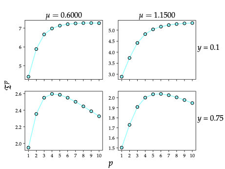
In summary, the study of the CDARN() model in the limit of no-cross correlations provides us with a good understanding of the causes for two of the most notable phenomena observed in the full network systems, and allows us to focus on the role of correlations in inducing the remaining effects.
V.4 Derivation of the temporal correlation matrix
We will now present a general analytical approach to finding the lagged cross and autocorrelations for an arbitrary coupling matrix , which we will use in Section V.5 to explore the interplay between correlations and memory in more depth than would be possible through simulations alone. In particular, we will use it to isolate the effects that correlations among neighbouring links in the LCC coupling model have on the time taken for diffusion processes on the temporal network to reach equilibrium.
The results of Section V.2 clearly indicate that the presence of coupling in the temporal dynamics of different links plays an important role in the behaviour of the rescaled time to equilibrium for a diffusion process on a temporal network. Indeed our claim is that, while the temporal autocorrelations of links slow down diffusion Masuda et al. 2013; Scholtes et al. 2014; Rosvall et al. 2014; Hiraoka and Jo 2018; Jo et al. 2015, as evidenced by the limit of no cross correlations case, temporal correlations among neighbouring links speeds it up. Fortunately, the CDARN() model is analytically tractable enough for us to fully describe the correlations that are present for a general coupling matrix , without relying wholly on simulations.
Rather than working with the backbone network directly, we will instead consider the corresponding graph in which links are the nodes in the backbone, and we connect any two nodes in the new graph if their links in the backbone graph shared a node. For a backbone network with possible links, we assign each of these links with a linear index. Then let us denote the correlations between link and at time lag as . Given a coupling matrix , can be found as the solution to the following Yule-Walker equations Jacobs and Lewis 1978a; MacDonald and Zucchini 1997:
| (21) |
Note that we have dropped our indices, and so each element in the equation is a matrix. We can show that, for general , this equation is solved by the composition of different functions over supports for integer . The first of these can be found to be constant, while the following are exponentially decaying (see Appendix J, K). Because of this, we can characterise the correlations at all values of in terms of this initial constant, which we call . We first define the following tensor:
| (22) |
then can be found as the solution to the following system of linear equations (see Appendix J)
| (23) |
The system can be greatly simplified in special cases (see Appendix K, L, M, N). For example, in the case of the UCC coupling model, we show that is constant for all , and similarly is constant for all pairs such that , thus reducing the calculation of the correlation coefficients to solving a pair of linear simultaneous equations. Given this set of equations for , we can also then find the correlations when as
| (24) |
This gives us a full picture of the correlations present in the CDARN() model and allows us to calculate them directly.
V.5 Cross-interactions speed up the diffusion
We saw in our study of diffusion in the limit of no cross correlations that the rescaled time to equilibrium is a non-monotonic function of the memory length . It is also widely understood that a way of characterising memory of a time series is by using the autocorrelation function. We find for a CDARN() process the memory is precisely the value for the time lag after which the correlation function decays exponentially (see Appendix H and results in Williams et al. 2019). With this in mind we can now focus on the comparison between autocorrelation coefficients of links in a CDARN() temporal model and the cross correlation coefficients of neighbouring links. This is done by studying the constant values for the auto and cross correlation coefficients at time lags . In order to do this effectively for large networks we will average these quantities over all links (and neighbours where appropriate) to gain the averaged autocorrelation coefficient and the averaged neighbourhood correlation coefficient . These are defined, given the matrix of correlation coefficients for a backbone with links derived in Section V.4, as
| (25) |
where as before is the set of links in the neighbourhood of
on the network backbone .

For clarity, let us now re-state our claim, as based on our observations of the numerical simulations displayed in Fig. 8: while autocorrelation of links slows down diffusion, correlations between neighbouring links speeds up diffusion. While in Fig. 8 we do see that diffusion is faster in the LCC model than in the NCC model, the autocorrelations of links in the two models are different. Further to this, while it would be possible to tune the parameters of the NCC model so that it produced links with the same autocorrelation coefficient as the LCC model, as the NCC model does not have a coupling strength, this could only be achieved by changing either the memory strength or the memory length . Because of this we can not judge the influence of neighbourhood correlations from our previous results, and we cannot use the NCC model to explore the effects of neighbourhood correlations further. In order to give a valid point of comparison, we can now make use of our third coupling model, which allows us to precisely control the average link autocorrelation, but also removes any correlations between neighbouring links. To recall, for a backbone with links, the coupling matrix in the UCC model is given by . The simplicity of this model lends itself well to analytical calculations, and so we can now use this model to isolate the effects of neighbourhood correlations. Indeed we can show that in the limit of large numbers of links this model reduces to a DARN() temporal network on a fixed backbone, in which links are independent (see Appendix N). First we fix the parameters and for both the LCC and UCC models, this ensures that there is the same memory strength and length, and the average degree of the temporal networks produced are the same. We can then fix the value of for the LCC model, as shown in Fig. 10 (first row), and calculate the resulting value of and , as defined by Eq. 22,23 and 25. By then varying the value of used in the corresponding UCC model we obtain precisely the same value for , while leaving , because in the considered network backbones the number of links is large. In figure 10 we plot both the values for and , along with the rescaled time till equilibrium for a diffusion process on the corresponding temporal network. Note that the LCC and UCC models have, by construction, exactly the same value of , and so only LCC is plotted in the upper panels, and the NCC model must always have , and so it is not plotted in the lower panels.
We observe here that, as expected, the value of in the NCC model is significantly higher than for the LCC model. We also see that both and decay as the memory length increases, consistent with the DARN() temporal network model. Most notably, there are significant differences between the values of given for each backbone. While both the Airport and Tube backbones display significant neighbourhood correlations in the LCC coupling model (though the values are larger for the Tube backbone), the Emails backbone only has notable neighbourhood correlations for low values of , and indeed at is practically indistinguishable from the NCC model. Also, as expected the value of for the UCC model is always approximately 0. We have tested our hypothesis by comparing the rescaled time to equilibrium (see the lower two rows of Fig. 10) for both the LCC and UCC models, both generated and plotted in exactly the same way as was done for Fig. 8. It is clear that when the value of is large, as in the Tube backbone, diffusion on the LCC coupling model is always faster. When is lower, as in the Airports backbone, this is still true. Finally, when there are little to no correlations between neighbours, as with the Email backbone, diffusion on the LCC coupling model is only faster than on the UCC model for small values of , after this point the value of is so small that its effects are no longer apparent. While the results for the Email backbone indicate that correlations among neighbours are not the only influence on behaviour, it is clear that their presence does act to speed up diffusion processes over the temporal network.
VI Conclusions
The influence that memory in temporal networks has on the link dynamics of the networks themselves as well as on processes that run on them is increasingly seen as key to our understanding of the way that our highly networked world operates. In the context of spreading processes on temporal networks, such as the passage of infections or the diffusion of information, it has been observed that the presence of memory can either speed up or slow down the spreading relative to some memoryless case. This result has been observed here in a manner reminiscent of other recent findings. What is generally less well understood is precisely how memory causes this change in the speed of spreading and the role of the multivariate structure of interactions of the link dynamics. A great deal of work has gone into the studying of how the correlated bursts in link activity that are the result of non-exponential inter link times, and hence memory, slow down spreading processes. This however does not yet give us a full picture.
Here we have introduced a novel, flexible and controllable generative model for temporal networks which allows for arbitrary backbone topologies, and precise control over the memory strength, memory length, average degree, and coupling strength. The new model can be interpreted as the temporal generalisation of the Erdős-Renyi random graph with non-Markovian memory, backbone structure, and both self- and cross- interactions of links. Not only this, but the model is simple enough to allow applications to empirical data by using maximum likelihood estimation methods.
Hence, first of all, we have empirically proved that, despite the simplicity of the model, it is possible to infer many memory patterns observed in the real world. By estimating the model on a number of datasets, we have shown that: transportation networks are Markovian systems with significant cross-correlations of links capturing the presence of transport connections between the physical nodes, i.e. stops, of the network; social networks (both online and offline) are in general non-Markovian with a memory order larger than one, and display auto-correlations of links, as a result of the stability pattern characterising some social ties, such as friendship; football networks are Markovian and display both link-specific persistence and cross interactions between links, with the two memory patterns which are inversely correlated as functions of the time resolution, as a result of the underlying contact dynamics of the game. Finally, within our framework, we have further validated the importance of describing the cross-interactions of links with a study of link prediction, thus showing how we are able to improve significantly the forecasting performance when such effects are included.
The model is rich but flexible enough to allow the analytical treatment of a number of theoretical problems, including finding the exact correlations between any two links. Given this we have been able to study exactly how the memory and coupling of the dynamics of different links in our model influence a spreading processes on the network. In doing this we have provided a solution to the time taken for a diffusion process to reach equilibrium in the limit of no cross correlations and as a function of the memory length . This shows us that the spreading time is non-monotonically dependent on , and allows us to infer that the equivalent memoryless process provides the fastest possible diffusion in our model. Looking at networks we have shown that correlations play a subtler role than might previously been expected. While we find, in accordance with previous works, that non-exponentially decaying autocorrelations among links do slow down diffusion, we, surprisingly, see that the opposite is true of local correlations. When links that share a node are correlated, this tends to speed up diffusion. This is made clear by the fact that when we observe a system in which links have fixed autocorrelation, but the correlations between neighbouring links varies (while all other parameters are kept constant), then diffusion is faster when correlations among neighbours are higher. This has strong implications for real world systems. While it is understood that memory and correlations between links have an effect on the spreading of information, the observation that correlations between neighbours and autocorrelations behave in opposite ways directly contributes to our understanding of many empirical systems. For example, when considering the diffusion of information over a social network, and any consequent formation of opinions, correlations between two different social ties must be considered as important as the correlation of a social tie with its own history. In a more general sense our findings also suggest that considering the evolution of links as independent processes in a temporal network means we loose a significant amount of information. Hence, when assessing the properties of an empirical network, correlations between the evolutions of links must be taken into account. Finally, we have been able to test our model using as backbones the topologies of real-world systems. The differences in spreading behaviour demonstrated among these backbones show the important role that such topologies play. It is clear that memory, correlations and backbone interact in a complex manner, and when considering the study of real world systems one can not assume to study of any of these features in isolation. Here, however, we have provided a framework in which the interplay between these features can be studied systematically, and how surprising results occur when we do.
Acknowledgements.
VL work was funded by the Leverhulme Trust Research Fellowship “CREATE: the network components of creativity and success”. FL and PM acknowledge support by the European Integrated Infrastructure for Social Mining and Big Data Analytics (SoBigData++, Grant Agreement #871042). We also thank Lucas Lacasa for useful discussions.Author contributions
All the authors designed the research. O.W. and P.M. performed calculations and generated figures. All the authors discussed intermediate and final results and wrote the paper.
Competing interests
The authors declare no competing interests, financial or otherwise.
Correspondance
Correspondence and requests for materials should be addressed to O.W or V.L.
Open-source software
The codes for both simulation and estimation of the CDARN(p) models proposed in this paper are available online at http://www.sobigdata.eu/.
VII Appendix
VII.1 Linear indexing for links
Throughout this work we frequently make use of a linear indexing for links in a network, and, equivalently, entries in a matrix. In practice this is a way to take a pair of indices for either network nodes, or rows and columns of the adjacency matrix, say , and map it to a single number . As only requirement we need for such a mapping to be bijective, that is each unique pair corresponds to a unique value . As an example, the simplest way this can be done, assuming for some value , is to take element of a matrix as 1, then proceeding left to right line by line.
VII.2 Average degree of the CDARN() network
Our aim is to show that a CDARN() network on a complete backbone has the same average degree as a DARN() network, and hence as an Erdős-Renyi (ER) random graph. To do this we need only show that the average value of an arbitrary link is given by . Let us proceed by first averaging over the left and right hand sides of Eq. 4 to get
| (26) |
where the symbols denote temporal averages. If we now label the link with its linear index , we obtain the following
| (27) |
where are the entries of the coupling matrix . In the above we have made use of the stationarity of the sequence to say that . One can see also that , for some constant , is a solution to the above equations. The fact that is row stochastic, and so its rows sum to 1, then gives us that is the unique solution. Hence, we have obtained , that is we have shown that the CDARN() produces networks with the same average degree of the DARN() model.
VII.3 The infinite memory limit
One of the key features of the DARN() model is that, as , it produces temporal networks that are indistinguishable from a sequence of independent ER graphs. Our aim now is to show that this is true for the CDARN() model as well. We start by writing the conditional probability for a single link with linear index :
| (28) |
where is the random matrix representing the adjacency matrix at time , which we say has observed values . We hence see that our problem can be reduced to a study of the properties of some kernel function , defined as the probability that a 1 is drawn from any point in the memory, i.e.
| (29) |
We recognise the sample expectation over the past steps of the time series, and so can see that as . For completeness we must also check that any fluctuations away from the mean can be ignored at finite times. First we see the following
| (30) |
We then have that , and so
| (31) | |||
| (32) |
Hence, in the large limit then the memory kernel tends to 0, and so the system is equivalent to one in which there is no memory. This displays exactly the same behaviour as is found for the DARN() model: the CDARN() model does indeed tend to a memoryless model in the limit of large memory. In the memoryless case we note that , and so must have an expected inter-link time of , and correspondingly the expected time until the th link is .
VII.4 Time to equilibrium in a two node system with a permanent link
Consider the equations defining diffusion in continuous time between two nodes, for which the link between them is permanent (always present):
| (33) |
If we impose conservation, i.e. , (and drop the 1 so that ) we can rewrite this as
| (34) |
Assuming , the solution is
| (35) |
We say that this system has reached equilibrium at the first time (in a continuous sense) where for some small positive . Again, imposing conservation this can be rewritten as the first value of such that . With Eq. 35 we can then find the (continuous) time to equilibrium directly as
| (36) |
Hence the number of full time steps of length which must occur before equilibrium is reached is given by
| (37) |
Note that for this system, for any given values of and we can always find , meaning that we may fix and still recover the full range of possible values for by varying .
VII.5 The transition matrix for a DAR() variable
Consider a stochastic process where the random variable is governed by the the DAR() model:
| (38) |
where, for each , and are Bernoulli random variables, while picks integers uniformly from the set . This can be thought of as a -th order Markov chain, and so is equivalent to a first order Markov chain in an enlarged state space MacDonald and Zucchini 1997. Accordingly, we define the so-called “-state” of link at time , by combining the state of the link at time along with its previous states in the vector . If we now define the set as the set containing all possible -states, then for any we can look at the conditional probability . This defines the entries of the -th order transition matrix. More details on the transition matrix of the DAR() model can be found in Williams et al. 2019.
VII.6 State indexing
When writing the matrix element we are implicitly associating an index to the states and . Since elements of a matrix are usually labeled by values (or ) for some value of , we must hence impose an ordering on the states . This is done by associating a linear index to each possible state (and similarly for ). The simplest form of this labelling function in our case, given a memory length of , is
| (39) |
where is the entry in the -state vector associated with . In practice this is equivalent to consider the sequence of 0’s and 1’s, representing the link history corresponding to state , as a binary number and converting in into to a decimal number. We will implicitly assume that wherever we use , or any state in , we are referring to the label , and that the labelling function is as given in Eq. 39.
VII.7 Initialising CDARN() model simulations
When generating realisations of the CDARN() model for the purposes of Monte-Carlo simulation (or any other simulation) it is important to ensure that the model is appropriately initialised. In all of the simulations and calculations here we require that the model be in a steady state, and so before any simulated diffusion starts we do the following:
- •
For each link and for each time assign to link state the value taken by a random variable . This gives us a set of pre-initial conditions from which simulation can be started.
- •
Simulate the CDARN() model for times using the previously generated states of the network, for some large . is chosen so that the network has reached a steady state, as approximated by the point where the autocorrelations have decayed below some suitable threshold. Functionally this has been set at approximately .
- •
Any simulation on top of the network can now start. This process must be repeated for every simulated realisation.
VII.8 Average time to equilibrium for a single Markov link
The value of the average time until diffusion across a single DAR(1) link reaches equilibrium, is central to any analysis of the rescaled times to equilibrium. Hence, we calculate it explicitly here. We know that, given the value from Eq. 37 giving the number of time steps until equilibrium in the two node system where the link is always present, will be precisely the time taken for a DAR(1) link to occur times. This can be found as the solution to the following equation:
| (40) |
where denotes the power of the matrix . Now will be a matrix, and and will be two dimensional vectors. Given the definition of as the probability that a system starting in state ends in state , we can easily see that the following must be true:
| (41) |
and so
| (42) |
Similarly we may find that and , and and . Giving us the equation
| (43) |
It is then a simple matter to extend this result and calculate the value of the rescaled time to equilibrium directly. Given that we know as , and this is precisely the value of , we then find:
| (44) |
It is easy to see that the maxima and minima of this function in terms of and are finite and occur at their limiting values ( and respectively) if . However in the limit we see that . In the limit we obtain the value , as expected.
VII.9 Rescaled time to equilibrium in the limit of large
In the main text we claim that for suitably sparse initial conditions, i.e. when is small, but that for the opposite can be true. To understand this we first formalise our statement: given an initial probability vector , we have , provided that the entries representing states in which no link is present (in our case for ) contain the majority of the probability mass. Recall first that we are implicitly labelling our states according to the labelling function given in Eq. 39. Now, notice that, since is a probability vector, and is a stochastic matrix, we can define a vector such that for all , and we can write the following equation:
| (45) |
Hence we can write
| (46) |
By construction if , and so if we define
| (47) |
then, when , we have . Hence, we see that if (the entry in representing an initial state with no links), then we need only check that to show that . This can be checked directly by analysing the average time taken to reach equilibrium , given some starting state , as defined by the following set of linear equations:
| (48) |
where . From this we can directly obtain
| (49) |
and hence confirm that when . We now want to understand the conditions in which this breaks down, and we instead observe . One can manually check that, for any values of or , for , but that this inequality does not generally hold for . As a specific example of this, if we fix , and , then , but . To understand this behaviour, we can then make use of the following two facts about . Given a memory state ,
- •
If by we indicate the memory state with a 1 in the th entry, and zeros elsewhere, then the values of are given by solutions to the equation , with appropriate values for and .
- •
if is the memory state obtained by taking memory state and replacing any of its 0 states with 1, then .
To prove the first of these statements, we directly analyse Eq. 48. This equation, in our notation becomes , but we also notice that is invariant of , always taking the value , which we will now denote as . To obtain the desired form of difference equation, we now simply identify and . This can be easily solved to give the following:
| (50) |
This equation must clearly be decreasing with n.
To prove the second of these statements consider two possible memory states and , where is given by taking and replacing one of the zeros in its memory with a one. Let us label the position of the state which we change with . Now let us now denote , where , and similarly for . To clarify, we can think of as being the memory state shifted back times, or similarly what happens to the memory state of a DAR() process if it starts in state and generates zeros. We can then write the following equation directly from Eq. 48:
| (51) |
Given our definition in Eq. V.3, and the fact that is with a 1 added, we can rearrange this to give
| (52) |
From this we can see that if then we must have . Now, by construction we know that , since this is the point at which the additional 1 in the memory is removed. In turn this means that . Inductively this gives us that
| (53) |
Thus we have that .
Hence we have proved that
is decreased by adding a one at any point in the memory,
and, equally, increased by adding a zero at any point in the memory.
The first statement gives us that, since we can not guarantee that
, we can not guarantee that, for any state with
a single one in any position other than 1, .
The second statement then tells us that, since any state
can be generated by taking a state with only a single 1 somewhere,
and adding more 1’s to it,
we can never guarantee that for any .
Because of this we see that for small we must have , and hence we must have , finally giving us that . However, for larger this may not be the case.
VII.10 Correlations in the CDARN() model
By introducing the possibility that a link in a DARN() network can draw from the memory of another link, and hence creating the CDARN() model, we have introduced correlations among the activities of different links. As we will show in this appendix, the extent of these correlations can be completely characterised analytically. If we have a network with possible links, each with its own linear index, let us denote the correlations between link and at time lag as . Following the procedures in Williams et al. 2019; Jacobs and Lewis 1978a, we can derive the Yule-Walker equations:
| (54) |
where the elements are taken from the coupling matrix assigning the probability of a link drawing from the memory of link . This can be written more compactly in terms of the corresponding matrices and as
| (55) |
These equations can be solved given a suitable closure. Following Williams et al. 2019, we can re-write this expression for values of as
| (56) |
for some value . This equation can be seen to have a constant solution , which satisfies:
| (57) |
Now we need to find a suitable expression for . We know that, by definition, . The off diagonal entries however are given by the Yule-Walker equation
| (58) |
But, we know that the value of must be a constant , and so the off-diagonal elements of will be the same as the off-diagonal elements of
| (59) |
Putting everything together we get the equation
| (60) |
This can be rearranged to give
| (61) |
This can be further simplified by constructing the tensor as
| (62) |
The system of equations given in Eq. 57 can then be written as
| (63) |
This form is more easily dealt with in numerical applications, as a simple dimensional reduction (flattening) yields a more traditional form for a system of linear equations. Importantly, this solution relies on no properties of the coupling matrix other than stochasticity, which it must have by definition. In special cases, such as those where coupling is uniform or symmetric, we can simplify these equations further by analysing the symmetries that arise in and .
VII.11 Evolution of the autocorrelation function
We wish to now show that the full extent of the autocorrelations in our model are described by the constant value , given over the first time steps. We first notice that from Eq. 55 we can obtain the following:
| (64) |
and hence
| (65) |
However, we know that for the autocorrelation is a constant , meaning that for Eq. 65 becomes
| (66) |
This is now a first order inhomogeneous difference equation with solution
| (67) |
where is a constant matrix. By noticing that we obtain the expression
| (68) |
With this solution we see that the equation governing the values of , for in the range to , is of the form
| (69) |
where , , and are constant matrices. This equations has a general solution
| (70) |
where is a constant matrix, and is a matrix that is constant over every interval . Moreover, in our specific case we find that and . This implies that not only is the autocorrelation function for the CDARN() process exponentially decreasing for all values of larger than , but also that this decay varies according to a single parameter every time steps. This gives us a full picture of the autocorrelations for a CDARN() process.
VII.12 Special case: totally symmetric cross correlation
The simplest type of correlation in the CDARN() model occurs when the coupling matrix is such that , i.e. regardless of the pair of links in question. We can immediately notice that our tensor now takes the form:
| (71) |
which is invariant over the three indexes and . Consequently must be invariant over and . Hence all of the lagged correlations have the same value, and we can write and , giving us the following equation:
| (72) |
Solving for gives
| (73) |
This provides a full picture of the lagged correlations present in the system. All that remains is to find the time 0 correlations when . This can be done as follows:
| (74) |
Where the last line is given by the fact that for we have , the constant value given in Eq. 73. Hence when , .
Note first that if then we recover the autocorrelation function of a DAR() process. Also note that as increases this value must decrease, meaning that for large networks both correlations and autocorrelations are removed, and so memory no longer has any effect on the evolution of the system.
VII.13 Special case: Uniform Cross Correlation (UCC)
The second special case we will consider is that of uniform cross correlation (UCC), as induced by a symmetric coupling matrix. Specifically this means that we require that be symmetric, with for all values of and some given value of , and for with . Going back to the general case in Eq. 63 we notice that these conditions ensure that is invariant with respect to , and when is invariant with respect to and . This means that all of the values of can be found as the solutions to the two following equations (note that is assumed here)
| (75) |
Hence we need only find the relevant values of to proceed. Given the definition of and and we can find the following:
| (76) |
Noticing that and are invariant of and (down to excluded values) we then obtain the following pair of equations:
| (77) |
This gives us a simple, solvable pair of equations. Note that while the full solution in terms of and is easy to obtain now, we will not write it down here due to its length. To find the time 0 correlations we can use Eq. 59 to obtain
| (78) |
Competing the description of the correlations for the UCC model.
VII.14 Uniform cross correlation in the large network limit
The uniform cross correlation (UCC) model for CDARN() networks was introduced to evenly distribute any temporal cross correlations between links over the entire network. In doing this we minimise the cross correlations, i.e. where , for fixed values of and . In turn this minimises the influence that any such cross correlations have on the diffusion process over the network. What we now show is that when the backbone of the temporal network has a large number of links then the UCC model is indistinguishable from a DARN() model that has been restricted to the same backbone, and hence temporal cross correlations between links are completely removed.
Consider a temporal network given by time varying adjacency matrix with observed value , and with links, generated by the CDARN() model with link density , memory strength , memory length and coupling matrix as in the UCC case. The conditional probability of a link occurring at time , given the past states of the network can be thought of in terms of contributions from the memory of the link itself, the memory of all other links, and some background contribution. This can hence be written as follows
| (79) |
where and represent the contributions to
the conditional probability
from the past states of the link and every
other link respectively.
For links to be effectively independent
then we require that as , tends to a
constant, and hence the link has no memory of the past states of
any other link. To show this we study the memory kernels
and directly as:
| (80) |
We need only focus on . First, let us consider the average value . The CDARN() network is taken to be in a stationary state, and so the symmetry of the links under any relabelling guarantees us that is the same for each link and for each time . Hence we can write for some constant . Then we must have, for any of the possible values of ,
| (81) |
Now, can be re-written as follows:
| (82) |
Then, by the law of large numbers we can express this in terms of the sample average:
| (83) |
Hence as . Indeed, we can further see that . Since there are no terms containing links other than in , then we can conclude that the conditional probability is such that, in the same limit ,
| (84) |
and so any memory of other links is lost. To show that this is equivalent to a DARN() network we need only look at the conditional probability of obtaining a link in such a network with memory strength , memory length , link density and adjacency matrix with observed values :
| (85) |
Now, by setting the values of and , in terms of the values , and from the CDARN() model, to be
| (86) |
we obtain that
| (87) |
Hence the UCC model is precisely a DARN() model in the limit of .
VII.15 MLE of the CDARN(p) model
The CDARN(p) model can be estimated by the maximum likelihood method. First of all, consider the vectorization , with the number of links on the backbone, of the adjacency matrix of the network snapshot at time . That is, describes the binary random sequences associated with the dynamics of the links on the backbone. Then, the log-likelihood of data (by conditioning on the first observations) under CDARN(p), as defined in Section IV, reads as:
| (88) |
where runs from to , while from to , with
where is the Kronecker delta, taking value equal to one if , zero otherwise, is the probability of picking in the range of integers (it is if we assume uniform probability), and is:
- 1.
with , for the no cross correlation (NCC) coupling model;
- 2.
with the number of neighbours of link if , zero otherwise, for the local cross correlation (LCC) coupling model;
- 3.
with , for the uniform cross correlation (UCC) coupling model.
The MLE of the CDARN(p) model can be then obtained by maximising the log-likelihood in Eq. (88), or, equivalently, by solving the following system of non-linear equations:
| (89) |
The system of non-linear equations can be solved iteratively by adopting an iterative proportional fitting procedure. This consists in solving one by one each equation for each parameter, but conditioning on the values of the other parameters, up to convergence. Such procedure can be initialized randomly in the parameter space, however a natural initialization for the parameter is the average link density of the network. For further details on the method see also Mazzarisi et al. 2020a.
VII.16 MLE of the heterogeneous CDARN(p) model
In the case of link-specific parameters or with , the log-likelihood of data under CDARN(p) with heterogenous parameters is generalized quite naturally as
| (90) |
and
| (91) |
respectively for and . Then, similarly to before, the MLE of the CDARN(p) model with heterogenous parameters is obtained by solving
| (92) |
and
| (93) |
respectively.
VII.17 Link prediction in the CDARN(p) model
Once estimated on data by solving the MLE problem (6), the CDARN(p) model can be used for link prediction: assume that we observe a temporal network up to time and are asking for the prediction of the network snapshot at time (by using only the information up to time ). The one-step-ahead forecast (or prediction) of link is defined as
| (94) |
with
The one-step ahead forecast in Eq. (94) is described by a real value in the unit interval, representing the probability projected at time of observing a link, then the prediction itself, namely the binary value , is obtained according to some threshold value. The time series of forecasts , together with the realisations , allow us to characterise the forecasting performance of the model by using some binary classifier. A possibility is constructing the Receiving Operating Characteristic (ROC) curve Hastie et al. 2009, which is the plot of the True Positive Rate (TPR) (sensitivity) against the False Positive Rate (FPR) (specificity) at various threshold values of the link probability. In particular, the threshold values are selected implicitly by the inputs themselves: by moving from zero to one in the unit interval, each time the sensitivity is increasing or the specificity is decreasing, the corresponding value is considered as a threshold. In practical terms, the better the model performs in the forecasting, the higher the associated ROC curve is in the unit square, or, equivalently, the larger the Area Under the Curve (AUC).
VII.18 Network statistics
Once estimated on data, the CDARN(p) model in the standard version with constant parameters and for a specific coupling specification, captures the average link density of a temporal network, together with the average auto- and cross-correlations of links, in particular the cross-correlations of links interacting on the backbone, e.g. all links that are incident to the same nodes (neighbours links) for the LCC specification. Thus, the observed statistics match (on average) their expectations according to the CDARN(p) model, eventually computed by using simulations. For validation purpose, this is shown in Fig. 11 for all the datasets described in Section IV by considering the CDARN(1)-LCC model with constant parameters, which are estimated on data by using maximum likelihood methods described above.

More interestingly, other networks statistics that are not explicitly described by CDARN models, can be computed within the proposed framework, in particular the inter-event time between the occurrence of two subsequent links between two nodes at two different times. For instance, for temporal networks of human communication, it has been observed that the duration between two contacts is often bursty, deviating from a uniform distribution expected by some memoryless process Holme and Saramäki 2012. This quantity is of great interest, e.g. , when studying any spreading process taking place on temporal networks, such as diffusion as in the present work. In our setting, the inter-event time can be defined as the number of observed time snapshots for which the generic link is zero, after an observation . The distribution of conditional to the observation for the CDARN(1) model (with constant parameters) is equivalent to compute the following joint probability
| (95) | |||
with .
In general, a closed form solution cannot be obtained because of non-diagonal interaction terms mediated by the couplings matrix . Except for the NCC specification of the model, i.e. the DARN(1) model, which sets to zero the cross-correlations, i.e. . In this case, the probability distribution of the inter-event time is
| (96) |
with , as follows from simple computations.
Notice that the probability distribution (96) of the DARN(1) model represents an upper bound for the CDARN(1) model: when in Eq. (95), there exists always a probability larger than zero of copying one past neighbour link (whatever the coupling matrix ), instead of copying the past itself, i.e. a zero, with probability one. This reduces the probability of observing a number of successive zeros, thus resulting in an (approximate) exponential distribution of inter-event times with a time scale smaller than , see the left panel of Fig. 12. Finally, the non-Markovian case is not analytically tractable as long as increases further and further. However, for the NCC specification of the CDARN(p) model, i.e. DARN(p), it is easy to gather that when , by following similar computations leading to Eq. (95). This is confirmed numerically in the right panel of Fig. 12. We can conclude that the inter-event time distribution of the CDARN(p) model is approximate exponential with a time scale equal or smaller than .


Finally, in Fig. 13 we show the empirical distribution of the inter-event time of four real-world temporal networks, compared with the corresponding distribution for the CDARN(1) model with coupling specification, obtained numerically by means of simulations, and with the theoretical one (96) for the DARN(1) model. In both cases, the parameters of the model has been obtained by maximum likelihood estimation. In all cases, the CDARN(1) can be seen as an approximation of the empirical distributions of the inter-event time for small , while the fatter tails (excluding the football network) are not captured by the model.

References
- González et al. (2008) M. C. González, C. A. Hidalgo, and A.-L. Barabási, Nature 453, 779 EP (2008).
- Starnini et al. (2013) M. Starnini, A. Baronchelli, and R. Pastor-Satorras, Physical Review Letters 110, 168701 (2013).
- Yoneki et al. (2009) E. Yoneki, D. Greenfield, and J. Crowcroft, in 2009 International Conference on Advances in Social Network Analysis and Mining (2009) pp. 356–361.
- Murcio et al. (2015) R. Murcio, A. P. Masucci, E. Arcaute, and M. Batty, Physical Review E 92, 062130 (2015).
- Li et al. (2015) D. Li, B. Fu, Y. Wang, G. Lu, Y. Berezin, H. E. Stanley, and S. Havlin, Proceedings of the National Academy of Sciences 112, 669 (2015).
- Mazzarisi et al. (2020a) P. Mazzarisi, P. Barucca, F. Lillo, and D. Tantari, European Journal of Operational Research 281, 50 (2020a).
- Valencia et al. (2008) M. Valencia, J. Martinerie, S. Dupont, and M. Chavez, Physical Review E 77, 050905 (2008).
- Fallani et al. (2008) F. D. V. Fallani, V. Latora, L. Astolfi, F. Cincotti, D. Mattia, M. G. Marciani, S. Salinari, A. Colosimo, and F. Babiloni, Journal of Physics A: Mathematical and Theoretical 41, 224014 (2008).
- Millán et al. (2018) A. P. Millán, J. Torres, S. Johnson, and J. Marro, Nature Communications 9, 2236 (2018).
- Chialvo (2010) D. R. Chialvo, Nature Physics 6, 744 (2010).
- Grindrod and Higham (2010) P. Grindrod and D. J. Higham, Proceedings of the Royal Society of London A: Mathematical, Physical and Engineering Sciences 466, 753 (2010).
- Holme and Saramäki (2012) P. Holme and J. Saramäki, Physics Reports 519, 97 (2012), temporal Networks.
- Masuda and Lambiotte (2016) N. Masuda and R. Lambiotte, A Guide to Temporal Networks (World Scientific (Europe), 2016).
- Gauvin et al. (2014) L. Gauvin, A. Panisson, and C. Cattuto, PloS one 9, e86028 (2014).
- Zanin et al. (2009) M. Zanin, L. Lacasa, and M. Cea, Chaos: An Interdisciplinary Journal of Nonlinear Science 19, 023111 (2009).
- Nicosia et al. (2012) V. Nicosia, J. Tang, M. Musolesi, G. Russo, C. Mascolo, and V. Latora, Chaos: An interdisciplinary journal of nonlinear science 22, 023101 (2012).
- Weng et al. (2017) T. Weng, J. Zhang, M. Small, R. Zheng, and P. Hui, Scientific reports 7, 41951 (2017).
- Peixoto and Rosvall (2017) T. P. Peixoto and M. Rosvall, Nature Communications 8, 582 (2017).
- Buscarino et al. (2008) A. Buscarino, L. Fortuna, M. Frasca, and V. Latora, EPL (Europhysics Letters) 82, 38002 (2008).
- Starnini and Pastor-Satorras (2014) M. Starnini and R. Pastor-Satorras, Physical Review E 89, 032807 (2014).
- Karsai et al. (2014) M. Karsai, N. Perra, and A. Vespignani, Scientific reports 4, 4001 (2014).
- Alessandretti et al. (2017) L. Alessandretti, K. Sun, A. Baronchelli, and N. Perra, Physical Review E 95, 052318 (2017).
- Singer et al. (2014) P. Singer, D. Helic, B. Taraghi, and M. Strohmaier, PLOS ONE 9, 1 (2014).
- Szell et al. (2012) M. Szell, R. Sinatra, G. Petri, S. Thurner, and V. Latora, Scientific Reports 2, 457 EP (2012).
- Lambiotte et al. (2019) R. Lambiotte, M. Rosvall, and I. Scholtes, Nature Physics , 1 (2019).
- Moinet et al. (2018a) A. Moinet, A. Barrat, and R. Pastor-Satorras, Physical Review E 98, 022303 (2018a).
- Zhang et al. (2017) Y. Zhang, A. Garas, and I. Scholtes, arXiv preprint arXiv:1701.06331 (2017).
- Salnikov et al. (2016) V. Salnikov, M. T. Schaub, and R. Lambiotte, Scientific reports 6, 23194 (2016).
- Matamalas et al. (2016) J. T. Matamalas, M. De Domenico, and A. Arenas, Journal of The Royal Society Interface 13, 20160203 (2016).
- Rosvall et al. (2014) M. Rosvall, A. V. Esquivel, A. Lancichinetti, J. D. West, and R. Lambiotte, Nat. Commun. 5, 4630 (2014).
- Hiraoka and Jo (2018) T. Hiraoka and H.-H. Jo, Scientific Reports 8, 15321 (2018).
- Sapienza et al. (2018) A. Sapienza, A. Barrat, C. Cattuto, and L. Gauvin, Physical Review E 98, 012317 (2018).
- Kiss et al. (2015) I. Z. Kiss, G. Röst, and Z. Vizi, Physical review letters 115, 078701 (2015).
- Peixoto and Gauvin (2018) T. P. Peixoto and L. Gauvin, Scientific reports 8, 15511 (2018).
- Williams et al. (2019) O. E. Williams, F. Lillo, and V. Latora, New Journal of Physics 21, 043028 (2019).
- Moinet et al. (2018b) A. Moinet, R. Pastor-Satorras, and A. Barrat, Physical Review E 97, 012313 (2018b).
- Masuda et al. (2013) N. Masuda, K. Klemm, and V. M. Eguíluz, Physical Review Letters 111, 188701 (2013).
- Delvenne et al. (2015) J.-C. Delvenne, R. Lambiotte, and L. E. Rocha, Nature Communications 6, 7366 (2015).
- Scholtes et al. (2014) I. Scholtes, N. Wider, R. Pfitzner, A. Garas, C. J. Tessone, and F. Schweitzer, Nature Communications 5, 5024 (2014).
- Zhan et al. (2019) X.-X. Zhan, A. Hanjalic, and H. Wang, Scientific reports 9, 6798 (2019).
- Jo et al. (2015) H.-H. Jo, J. I. Perotti, K. Kaski, and J. Kertész, Physical Review E 92, 022814 (2015).
- Burioni et al. (2017) R. Burioni, E. Ubaldi, and A. Vezzani, Journal of Statistical Mechanics: Theory and Experiment 2017, 054001 (2017).
- Kim et al. (2015) H. Kim, M. Ha, and H. Jeong, The European Physical Journal B 88, 315 (2015).
- Georgiou et al. (2015) N. Georgiou, I. Z. Kiss, and E. Scalas, Physical Review E 92, 042801 (2015).
- Scholtes (2017) I. Scholtes, in Proceedings of the 23rd ACM SIGKDD International Conference on Knowledge Discovery and Data Mining (ACM, 2017) pp. 1037–1046.
- Lambiotte et al. (2015) R. Lambiotte, V. Salnikov, and M. Rosvall, Journal of Complex Networks 3, 177 (2015).
- Vestergaard et al. (2014) C. L. Vestergaard, M. Génois, and A. Barrat, Physical Review E 90, 042805 (2014).
- Colman and Vukadinovi ć Greetham (2015) E. R. Colman and D. Vukadinovi ć Greetham, Physical Review E 92, 012817 (2015).
- Van Mieghem and van de Bovenkamp (2013) P. Van Mieghem and R. van de Bovenkamp, Physical Review Letters 110, 108701 (2013).
- Perra et al. (2012) N. Perra, B. Gonçalves, R. Pastor-Satorras, and A. Vespignani, Scientific reports 2, 469 (2012).
- Hoff et al. (2002) P. D. Hoff, A. E. Raftery, and M. S. Handcock, Journal of the American Statistical Association 97, 1090 (2002).
- Sarkar and Moore (2005) P. Sarkar and A. W. Moore, Acm sigkdd explorations newsletter 7, 31 (2005).
- Starnini et al. (2016) M. Starnini, A. Baronchelli, and R. Pastor-Satorras, Social Networks 47, 130 (2016).
- Hanneke et al. (2010) S. Hanneke, W. Fu, E. P. Xing, et al., Electronic Journal of Statistics 4, 585 (2010).
- Campajola et al. (2021) C. Campajola, F. Lillo, P. Mazzarisi, and D. Tantari, Journal of Statistical Mechanics: Theory and Experiment 2021, 033412 (2021).
- Jacobs and Lewis (1978a) P. A. Jacobs and P. A. Lewis, Discrete Time Series Generated by Mixtures. III. Autoregressive Processes (DAR (p))., Tech. Rep. (NAVAL POSTGRADUATE SCHOOL MONTEREY CALIF, 1978).
- Jacobs and Lewis (1978b) P. A. Jacobs and P. A. Lewis, Journal of the Royal Statistical Society: Series B (Methodological) 40, 94 (1978b).
- Jacobs and Lewis (1978c) P. A. Jacobs and P. A. Lewis, Journal of the Royal Statistical Society: Series B (Methodological) 40, 222 (1978c).
- Jacobs and Lewis (1983) P. A. Jacobs and P. A. Lewis, Journal of Time Series Analysis 4, 19 (1983).
- Mazzarisi et al. (2020b) P. Mazzarisi, S. Zaoli, C. Campajola, and F. Lillo, Journal of Economic Dynamics and Control 121, 104022 (2020b).
- Hastie et al. (2009) T. Hastie, R. Tibshirani, and J. Friedman, The elements of statistical learning: data mining, inference, and prediction (Springer Science & Business Media, 2009).
- Min and Wynter (2011) W. Min and L. Wynter, Transportation Research Part C: Emerging Technologies 19, 606 (2011).
- Hamilton (1995) J. D. Hamilton, Economic Theory. II, Princeton University Press, USA , 625 (1995).
- Runge et al. (2015) J. Runge, V. Petoukhov, J. F. Donges, J. Hlinka, N. Jajcay, M. Vejmelka, D. Hartman, N. Marwan, M. Paluš, and J. Kurths, Nature Communications 6, 8502 EP (2015).
- Bollobás (2001) B. Bollobás, Random graphs, 73 (Cambridge university press, 2001).
- Williams et al. (2020) O. E. Williams, L. Lacasa, A. P. Millán, and V. Latora, arXiv preprint arXiv:2004.12784 (2020).
- Fan et al. (1998) J. Fan, M. Farmen, and I. Gijbels, Journal of the Royal Statistical Society: Series B (Statistical Methodology) 60, 591 (1998).
- (68) Here, the number of nodes is corresponding to the number of stations, or stops, characterizing the specific public transport at each city.
- Watts and Dodds (2007) D. J. Watts and P. S. Dodds, Journal of consumer research 34, 441 (2007).
- Schweitzer (2007) F. Schweitzer, Brownian agents and active particles: collective dynamics in the natural and social sciences (Springer, 2007).
- Di Matteo et al. (2003) T. Di Matteo, T. Aste, and S. Hyde, arXiv preprint cond-mat/0310544 (2003).
- Arenas et al. (2008) A. Arenas, A. Díaz-Guilera, J. Kurths, Y. Moreno, and C. Zhou, Physics Reports 469, 93 (2008).
- Boccaletti et al. (2006) S. Boccaletti, V. Latora, Y. Moreno, M. Chavez, and D.-U. Hwang, Physics reports 424, 175 (2006).
- Newman (2010) M. Newman, Networks: an introduction (Oxford university press, 2010).
- usa (2016) “Us airports network dataset – KONECT,” (2016).
- Michalski et al. (2011) R. Michalski, S. Palus, and P. Kazienko, in Lecture Notes in Business Information Processing, Vol. 87 (Springer Berlin Heidelberg, 2011) pp. 197–206.
- (77) T. for London, “Rolling origin and destination survey (rods),” .
- Cinlar (2013) E. Cinlar, Introduction to Stochastic Processes, Dover Books on Mathematics Series (Dover Publications, Incorporated, 2013).
- Ballester and Vorsatz (2014) C. Ballester and M. Vorsatz, Review of Economics and Statistics 96, 383 (2014).
- MacDonald and Zucchini (1997) I. L. MacDonald and W. Zucchini, Hidden Markov and other models for discrete-valued time series, Vol. 110 (CRC Press, 1997).