跳到论文正文
W Papers独立论文阅读器 arXiv:1909.08049 论文正文 计算阅读时间 · 0%
引用这篇论文根据当前论文元数据生成,正式投稿前建议核对。


License: arXiv.org perpetual non-exclusive license
arXiv:1909.08049v1 [cs.CV] 17 Sep 2019

Masked-RPCA: Sparse and Low-rank Decomposition Under Overlaying Model
and Application to Moving Object Detection

Amirhossein Khalilian-Gourtani Affiliation: Electrical and Computer Engineering Depatment, New York University. Correspondence to: akg404@nyu.edu    Shervin Minaee Affiliation: Expedia Inc.    Yao Wang Affiliation: Electrical and Computer Engineering Depatment, New York University.
Abstract

Foreground detection in a given video sequence is a pivotal step in many computer vision applications such as video surveillance system. Robust Principal Component Analysis (RPCA) performs low-rank and sparse decomposition and accomplishes such a task when the background is stationary and the foreground is dynamic and relatively small. A fundamental issue with RPCA is the assumption that the low-rank and sparse components are added at each element, whereas in reality, the moving foreground is overlaid on the background. We propose the representation via masked decomposition (i.e. an overlaying model) where each element either belongs to the low-rank or the sparse component, decided by a mask. We propose the Masked-RPCA algorithm to recover the mask and the low-rank components simultaneously, utilizing linearizing and alternating direction techniques. We further extend our formulation to be robust to dynamic changes in the background and enforce spatial connectivity in the foreground component. Our study shows significant improvement of the detected mask compared to post-processing on the sparse component obtained by other frameworks.

Keywords: 
Machine Learning, ICML

marginparsep has been altered.
topmargin has been altered.
marginparwidth has been altered.
marginparpush has been altered.

The page layout violates the ICML style.

Please do not change the page layout, or include packages like geometry, savetrees, or fullpage, which change it for you.

We’re not able to reliably undo arbitrary changes to the style. Please remove the offending package(s), or layout-changing commands and try again.

1 Introduction

Sparse and low-rank decomposition has been an active research area in signal and image processing in the past decade, with applications in motion segmentation (Cao et al. 2016), (Gao et al. 2014), image foreground extraction (Ebadi & Izquierdo 2016), and optics (Kafieh et al. 2015). In the simplest case, this problem can be formulated as:

minimizeL,Srank​(L)+λs​‖S‖0s.t.X=L+S,\underset{\mathchar 29004\mathchar 24891\mathchar 29011}{\text{minimize}}\quad\text{rank}\delimiter 67273472\mathchar 29004\delimiter 84054785\mathchar 8235\mathchar 28949_{\mathchar 29043}\delimiter 69645069\mathchar 29011\delimiter 69645069_{\mathchar 28720}\quad\text{s.t.}\quad\mathchar 29016\mathchar 12349\mathchar 29004\mathchar 8235\mathchar 29011\mathchar 24891 (1)

where L\mathchar 29004 and S\mathchar 29011 denote the low-rank and sparse components of the signal X\mathchar 29016, respectively. There are some situations in which a unique decomposition may not exist; e.g. if the low-rank matrix L itself is also very sparse, it becomes very hard to uniquely identify it from another sparse matrix. Therefore, there have been many studies to find the conditions under which this decomposition is possible, such as the works in (Candès et al. 2011), (Feng et al. 2013). Also because of the non-convexity of both the rank function and the ℓ0\mathchar 352_{\mathchar 28720} norm, the problem in (1) is NP-hard. In order to be able to solve this decomposition, usually the rank​(L)\text{rank}\delimiter 67273472\mathchar 29004\delimiter 84054785 is relaxed to ‖L‖∗\delimiter 69645069\mathchar 29004\delimiter 69645069_{\mathchar 8707} (the nuclear norm of L\mathchar 29004, which is the sum of its singular values), and the ‖S‖0\delimiter 69645069\mathchar 29011\delimiter 69645069_{\mathchar 28720} is relaxed by the ‖S‖1\delimiter 69645069\mathchar 29011\delimiter 69645069_{\mathchar 28721} approximation (Recht et al. 2010).

The dominant application of sparse and low-rank decomposition (aka RPCA) has been for moving object detection in videos (Chen et al. 2012), (Zhang et al. 2013), but it has also been used for various other applications. To name some of the prominent works, in (Peng et al. 2012), Peng et al proposed a sparse and low-rank decomposition approach with application for robust image alignment. A similar approach has been proposed by Zhang (Zhang et al. 2012) for transform invariant low-rank textures. In (Keshavan et al. 2010), Keshavan proposed an algorithm for matrix completion using low-rank decomposition.

There has been several improvement of the vanilla RPCA over the past decade, and despite their great improvements in terms of accuracy and speed, there is a fundamental limitation in most of these models. The basic assumption that all these models share is the additive model for the sparse and low-rank components. In reality, the dynamic foreground object is overlaid on top of the low-rank background. For a more detailed overview of RPCA extensions, we refer the readers to (Yazdi & Bouwmans 2018).

In this work, we try to address this issue by assuming a model for the case where the two components are overlaid on top of each other (instead of simply being added). Thus, each element of X\mathchar 29016 comes only from one of the components. Therefore, besides deriving the sparse and low-rank component we need to find their supports. Assuming W∈{0,1}m​n×k\mathchar 29015\mathchar 12850\left\{\mathchar 28720\mathchar 24891\mathchar 28721\right\}^{\mathchar 29037\mathchar 29038\mathchar 8706\mathchar 29035} denotes the support of S\mathchar 29011, we can write this overlaid signal summation as X=(1−W)∘L+W∘S\mathchar 29016\mathchar 12349\delimiter 67273472\mathchar 28721\mathchar 8704\mathchar 29015\delimiter 84054785\mathchar 8718\mathchar 29004\mathchar 8235\mathchar 29015\mathchar 8718\mathchar 29011. We can separate these components by assuming some prior knowledge on L\mathchar 29004, S\mathchar 29011 and W\mathchar 29015 terms, and forming an optimization problem. In fact, we do not need to even include the S\mathchar 29011 term in our optimization framework, since by having W\mathchar 29015, the S\mathchar 29011 component can easily be derived as S=W∘X\mathchar 29011\mathchar 12349\mathchar 29015\mathchar 8718\mathchar 29016. We propose an optimization algorithm (to be called M-RPCA) based on the alternating direction method of multipliers (ADMM) (Boyd et al. 2011) and ideas of linearizing (Lin et al. 2011). We show the convergence of the proposed algorithm to a Karush–Kuhn–Tucker (KKT) point under reasonable assumptions. Our experiments show that the proposed framework directly recovers the mask of the foreground without need for post processing on the sparse component as in the RPCA algorithm.

As with the original RPCA algorithm, the proposed M-RPCA algorithm has two limitations: 1) It does not enforce spatial connectivity of the foreground, and 2) when the background is not stationary and has random perturbations (such as water waves, moving leaves, etc.), these perturbations are usually picked up by the sparse component, leading to noisy foreground detection. We further show extensions of the proposed framework to tackle these problems. Following the idea of (Cao et al. 2016), we model the background as the sum of a low rank component and a sparse component (used to model the random perturbation in the dynamic background), and furthermore enforce the spatial connectivity of the foreground object by adding a total variation penalty on the mask in the optimization formulation. We propose an optimization algorithm (to be called extended M-RPCA or EM-RPCA) to solve for all three components and show that it leads to significant improvement over M-RPCA in sequences with dynamic background.

The idea of solving a masked decomposition problem was first proposed in (Minaee & Wang 2017) for image segmentation, where an image is considered to have two overlaid components (e.g. text overlaid on background), each modeled by a subspace. Here, we extend this work by assuming one component is low-rank, while the other is sparse.

The structure of the rest of this paper is as follows: Section II presents the problem formulation, and the proposed optimization framework to solve it, as well as a convergence analysis. Section III provides the detailed experimental results of the proposed framework for moving object detection, and its comparison with previous state-of-the-arts models. And finally the paper is concluded in Section V.

2 Problem Formulation and Solution

In this section we introduce the general framework of masked robust principal component analysis (Masked-RPCA) formulated as an optimization problem, propose an algorithmic solution based on ADMM and linearizing techniques, and investigate the convergence properties.

2.1 Masked Robust Principal Component Analysis

Given a sequence of video frames in X3​d∈ℝm×n×k\mathchar 29016^{\mathchar 28723\mathchar 29028}\mathchar 12850{\mathbb{\mathchar 29010}}^{\mathchar 29037\mathchar 8706\mathchar 29038\mathchar 8706\mathchar 29035} let us denote the matrix X∈ℝm​n×k\mathchar 29016\mathchar 12850{\mathbb{\mathchar 29010}}^{\mathchar 29037\mathchar 29038\mathchar 8706\mathchar 29035} which is constructed by vectorizing and stacking the frames of the video. Then, the goal is to recover the matrices L∈ℝm​n×k\mathchar 29004\mathchar 12850{\mathbb{\mathchar 29010}}^{\mathchar 29037\mathchar 29038\mathchar 8706\mathchar 29035} and W∈{0,1}m​n×k\mathchar 29015\mathchar 12850\left\{\mathchar 28720\mathchar 24891\mathchar 28721\right\}^{\mathchar 29037\mathchar 29038\mathchar 8706\mathchar 29035} such that W\mathchar 29015 denotes the foreground support and the low-rank matrix L\mathchar 29004 matches the video sequence X\mathchar 29016 wherever the foreground is not active. A plausible formulation of such problem can be written as (2).

minimizeL,W\displaystyle\underset{\mathchar 29004\mathchar 24891\mathchar 29015}{\text{minimize}} r​a​n​k​(L)+λw​ψ​(W)\displaystyle\rm{\displaystyle\mathchar 29042\mathchar 29025\mathchar 29038\mathchar 29035}\delimiter 67273472\mathchar 29004\delimiter 84054785\mathchar 8235\mathchar 28949_{\mathchar 29047}\mathchar 28960\delimiter 67273472\mathchar 29015\delimiter 84054785 (2)
subject to:\displaystyle\text{subject to:}
W∈{0,1}m​n×k\displaystyle\mathchar 29015\mathchar 12850\left\{\mathchar 28720\mathchar 24891\mathchar 28721\right\}^{\mathchar 29037\mathchar 29038\mathchar 8706\mathchar 29035}

where ψ⁡(⋅)\mathchar 28960\delimiter 67273472\mathchar 8705\delimiter 84054785 encodes our prior knowledge about W\mathchar 29015 and λw∈ℝ\mathchar 28949_{\mathchar 29047}\mathchar 12850{\mathbb{\mathchar 29010}} is the regularization parameter. The problem as stated in (2) is not tractable because 1) the general rank minimization problem is NP-hard (Recht et al. 2010), and 2) recovering the binary matrix W\mathchar 29015 requires solving a combinatorial problem. To manage the rank minimization in general, nuclear norm minimization is proposed as a surrogate especially in the context of matrix completion (Recht et al. 2010; Candès et al. 2011). Additionally, the W∈{0,1}m​n×k\mathchar 29015\mathchar 12850\left\{\mathchar 28720\mathchar 24891\mathchar 28721\right\}^{\mathchar 29037\mathchar 29038\mathchar 8706\mathchar 29035} constraint can be relaxed to the convex interval between zero and one, namely, W∈[0,1]m​n×k\mathchar 29015\mathchar 12850\left\delimiter 67482370\mathchar 28720\mathchar 24891\mathchar 28721\right\delimiter 84267779^{\mathchar 29037\mathchar 29038\mathchar 8706\mathchar 29035}. Imposing the sparsity of desired W\mathchar 29015 via ℓ1\mathchar 352_{\mathchar 28721}-norm we can formulate the problem as in (3).

minimizeL,W\displaystyle\underset{\mathchar 29004\mathchar 24891\mathchar 29015}{\text{minimize}} ‖L‖∗+λw​‖W‖1\displaystyle\delimiter 69645069\mathchar 29004\delimiter 69645069_{\mathchar 8707}\mathchar 8235\mathchar 28949_{\mathchar 29047}\delimiter 69645069\mathchar 29015\delimiter 69645069_{\mathchar 28721} (3)
subject to:\displaystyle\text{subject to:}
W∈[0,1]m​n×k\displaystyle\mathchar 29015\mathchar 12850\left\delimiter 67482370\mathchar 28720\mathchar 24891\mathchar 28721\right\delimiter 84267779^{\mathchar 29037\mathchar 29038\mathchar 8706\mathchar 29035}

The algorithm for solving the problem in (3) is not immediately apparent especially since the variables W\mathchar 29015 and L\mathchar 29004 are coupled. For general low-rank and sparse decomposition formulations the ADMM algorithm is shown to be effective (Candès et al. 2011). More recently, ADMM for multi-affine constraints under certain assumptions was introduced and analyzed (Goldfarb 2018). Additionally, ideas of linearizing such as Linearized Alternating Direction Method (LADM) for general affine constraint (Lin et al. 2011) and for nuclear norm minimization(Yang & Yuan 2013) were introduced to handle more complicated affine constraints. Here, we propose to use the linearizing techniques for the bi-affine constraint as in (3). This way not only we can deal with the coupling of the variables but also we will find closed form solution for each sub-problem of the ADMM algorithm.

In the following section we drive the steps of the algorithm by forming the augmented Lagrangian and minimizing the linearized augmented Lagrangian w.r.t. each variable. Let us denote the dual variable for the equality constraint by Ux\mathchar 29013_{\mathchar 29048} and abuse notation to show the indicator function over each element of matrix W\mathchar 29015 by ι[0,1]​(W)\mathchar 28947_{\left\delimiter 67482370\mathchar 28720\mathchar 24891\mathchar 28721\right\delimiter 84267779}\delimiter 67273472\mathchar 29015\delimiter 84054785 where ι (x)\mathchar 28947_{\mathchar 28682}\delimiter 67273472\mathchar 29048\delimiter 84054785 takes the value 0 if x∈Ω\mathchar 29048\mathchar 12850\mathchar 28682, otherwise infinity. The augmented Lagrangian can be written as in (4).

ℒ⁡(L,W,Ux)=‖L‖∗+λw​‖W‖1+ι[0,1]​(W)+⟨Ux,(1−W)∘(L−X)⟩+ρx2​‖(1−W)∘L−(1−W)∘X‖2\begin{split}\mathcal{\mathchar 29004}\delimiter 67273472\mathchar 29004\mathchar 24891\mathchar 29015\mathchar 24891\mathchar 29013_{\mathchar 29048}\delimiter 84054785&\mathchar 12349\delimiter 69645069\mathchar 29004\delimiter 69645069_{\mathchar 8707}\mathchar 8235\mathchar 28949_{\mathchar 29047}\delimiter 69645069\mathchar 29015\delimiter 69645069_{\mathchar 28721}\mathchar 8235\mathchar 28947_{\left\delimiter 67482370\mathchar 28720\mathchar 24891\mathchar 28721\right\delimiter 84267779}\left\delimiter 67273472\mathchar 29015\right\delimiter 84054785\\ &\mathchar 8235\delimiter 69632778\mathchar 29013_{\mathchar 29048}\mathchar 24891\delimiter 67273472\mathchar 28721\mathchar 8704\mathchar 29015\delimiter 84054785\mathchar 8718\delimiter 67273472\mathchar 29004\mathchar 8704\mathchar 29016\delimiter 84054785\delimiter 86414091\\ &\mathchar 8235{{\mathchar 28954_{\mathchar 29048}\over\mathchar 28722}}\delimiter 69645069\delimiter 67273472\mathchar 28721\mathchar 8704\mathchar 29015\delimiter 84054785\mathchar 8718\mathchar 29004\mathchar 8704\delimiter 67273472\mathchar 28721\mathchar 8704\mathchar 29015\delimiter 84054785\mathchar 8718\mathchar 29016\delimiter 69645069^{\mathchar 28722}\end{split} (4)
Definition 2.1.

For simplicity, let us define the following notation, where superscript i\mathchar 29033 denotes the iteration number.

ΛLi≜(1−Wi)∘((Li−X)∘(1−Wi)+UxiUNKNOWNx)\mathchar 28675^{\mathchar 29033}_{\mathchar 29004}\triangleq\left\delimiter 67273472\mathchar 28721\mathchar 8704\mathchar 29015^{\mathchar 29033}\right\delimiter 84054785\mathchar 8718\left\delimiter 67273472\delimiter 67273472\mathchar 29004^{\mathchar 29033}\mathchar 8704\mathchar 29016\delimiter 84054785\mathchar 8718\delimiter 67273472\mathchar 28721\mathchar 8704\mathchar 29015^{\mathchar 29033}\delimiter 84054785\mathchar 8235{{\mathchar 29013_{\mathchar 29048}^{\mathchar 29033}\over\mathchar 28954_{\mathchar 29048}}}\right\delimiter 84054785
ΛWi≜(X−Li+1)∘((Li+1−X)∘(1−Wi)+UxiUNKNOWNx)\mathchar 28675^{\mathchar 29033}_{\mathchar 29015}\triangleq\left\delimiter 67273472\mathchar 29016\mathchar 8704\mathchar 29004^{\mathchar 29033\mathchar 8235\mathchar 28721}\right\delimiter 84054785\mathchar 8718\left\delimiter 67273472\delimiter 67273472\mathchar 29004^{\mathchar 29033\mathchar 8235\mathchar 28721}\mathchar 8704\mathchar 29016\delimiter 84054785\mathchar 8718\delimiter 67273472\mathchar 28721\mathchar 8704\mathchar 29015^{\mathchar 29033}\delimiter 84054785\mathchar 8235{{\mathchar 29013_{\mathchar 29048}^{\mathchar 29033}\over\mathchar 28954_{\mathchar 29048}}}\right\delimiter 84054785
Definition 2.2.

Given matrix Y∈ℝm×n\mathchar 29017\mathchar 12850{\mathbb{\mathchar 29010}}^{\mathchar 29037\mathchar 8706\mathchar 29038} and δ>0\mathchar 28942\mathchar 12606\mathchar 28720, let Y=U​Σ​VT\mathchar 29017\mathchar 12349\mathchar 29013\mathchar 28678\mathchar 29014^{\mathchar 29012} and I\mathchar 29001 the identity matrix then, 𝒟⁡(Y,δ)=U​(Σ−δ​I)+​VT\mathcal{\mathchar 28996}\delimiter 67273472\mathchar 29017\mathchar 24891\mathchar 28942\delimiter 84054785\mathchar 12349\mathchar 29013\delimiter 67273472\mathchar 28678\mathchar 8704\mathchar 28942\mathchar 29001\delimiter 84054785_{\mathchar 8235}\mathchar 29014^{\mathchar 29012} where (a)+=max⁡{0,a}\delimiter 67273472\mathchar 29025\delimiter 84054785_{\mathchar 8235}\mathchar 12349\max\{\mathchar 28720\mathchar 24891\mathchar 29025\} denotes the singular value thresholding operator.

Definition 2.3.

Π[0,1]\mathchar 28677_{\left\delimiter 67482370\mathchar 28720\mathchar 24891\mathchar 28721\right\delimiter 84267779} denotes The projection onto the interval [0,1]\left\delimiter 67482370\mathchar 28720\mathchar 24891\mathchar 28721\right\delimiter 84267779.

The update for L\mathchar 29004 at each iteration is achieved by minimizing the linearized augmented Lagrangian while fixing the variables Wi\mathchar 29015^{\mathchar 29033} and Uxi\mathchar 29013_{\mathchar 29048}^{\mathchar 29033}:

Li+1=arg⁡minL​Γ​L​Γ∗+ρx2​Γ​(1−Wi)∘(L−X)+UxiUNKNOWNx​Γ2\begin{split}\mathchar 29004^{\mathchar 29033\mathchar 8235\mathchar 28721}\mathchar 12349\arg\min_{\mathchar 29004}\left\delimiter 0\mathchar 29004\right\delimiter 0_{\mathchar 8707}\mathchar 8235{{\mathchar 28954_{\mathchar 29048}\over\mathchar 28722}}\left\delimiter 0\delimiter 67273472\mathchar 28721\mathchar 8704\mathchar 29015^{\mathchar 29033}\delimiter 84054785\mathchar 8718\delimiter 67273472\mathchar 29004\mathchar 8704\mathchar 29016\delimiter 84054785\mathchar 8235{{\mathchar 29013_{\mathchar 29048}^{\mathchar 29033}\over\mathchar 28954_{\mathchar 29048}}}\right\delimiter 0^{\mathchar 28722}\end{split}

We can linearize the quadratic term as

12​Γ​(1−Wi)∘(L−X)+UxiUNKNOWNx​Γ2≃12​UNKNOWNL​‖L−Li‖2+⟨ΛLi,L−Li⟩+12​Γ​(Li−X)∘(1−Wi)+UxiUNKNOWNx​Γ2\begin{split}&{{\mathchar 28721\over\mathchar 28722}}\left\delimiter 0\delimiter 67273472\mathchar 28721\mathchar 8704\mathchar 29015^{\mathchar 29033}\delimiter 84054785\mathchar 8718\delimiter 67273472\mathchar 29004\mathchar 8704\mathchar 29016\delimiter 84054785\mathchar 8235{{\mathchar 29013_{\mathchar 29048}^{\mathchar 29033}\over\mathchar 28954_{\mathchar 29048}}}\right\delimiter 0^{\mathchar 28722}\mathchar 12839{{\mathchar 28721\over\mathchar 28722\mathchar 28956_{\mathchar 29004}}}\delimiter 69645069\mathchar 29004\mathchar 8704\mathchar 29004^{\mathchar 29033}\delimiter 69645069^{\mathchar 28722}\\ &\mathchar 8235\delimiter 69632778\mathchar 28675_{\mathchar 29004}^{\mathchar 29033}\mathchar 24891\mathchar 29004\mathchar 8704\mathchar 29004^{\mathchar 29033}\delimiter 86414091\mathchar 8235{{\mathchar 28721\over\mathchar 28722}}\left\delimiter 0\delimiter 67273472\mathchar 29004^{\mathchar 29033}\mathchar 8704\mathchar 29016\delimiter 84054785\mathchar 8718\delimiter 67273472\mathchar 28721\mathchar 8704\mathchar 29015^{\mathchar 29033}\delimiter 84054785\mathchar 8235{{\mathchar 29013_{\mathchar 29048}^{\mathchar 29033}\over\mathchar 28954_{\mathchar 29048}}}\right\delimiter 0^{\mathchar 28722}\end{split}

where τL>0\mathchar 28956_{\mathchar 29004}\mathchar 12606\mathchar 28720 is the proximal parameter. As a result the update rule for L\mathchar 29004 can be written as in (5).

Li+1=arg⁡minL⁡‖L‖∗+ρx2​UNKNOWNL​Γ​L−(Li−τL​ΛLi)​Γ2=𝒟⁡(Li−τL​ΛLi,τLUNKNOWNx)\begin{split}\mathchar 29004^{\mathchar 29033\mathchar 8235\mathchar 28721}&\mathchar 12349\arg\min_{\mathchar 29004}\delimiter 69645069\mathchar 29004\delimiter 69645069_{\mathchar 8707}\mathchar 8235{{\mathchar 28954_{\mathchar 29048}\over\mathchar 28722\mathchar 28956_{\mathchar 29004}}}\left\delimiter 0\mathchar 29004\mathchar 8704\left\delimiter 67273472\mathchar 29004^{\mathchar 29033}\mathchar 8704\mathchar 28956_{\mathchar 29004}\mathchar 28675_{\mathchar 29004}^{\mathchar 29033}\right\delimiter 84054785\right\delimiter 0^{\mathchar 28722}\\ &\mathchar 12349\mathcal{\mathchar 28996}\left\delimiter 67273472\mathchar 29004^{\mathchar 29033}\mathchar 8704\mathchar 28956_{\mathchar 29004}\mathchar 28675_{\mathchar 29004}^{\mathchar 29033}\mathchar 24891{{\mathchar 28956_{\mathchar 29004}\over\mathchar 28954_{\mathchar 29048}}}\right\delimiter 84054785\end{split} (5)

The update rule for W\mathchar 29015 is achieved by minimizing the linearized augmented Lagrangian while fixing Li+1\mathchar 29004^{\mathchar 29033\mathchar 8235\mathchar 28721} and Uxi\mathchar 29013^{\mathchar 29033}_{\mathchar 29048}. Using the same technique we have

12​Γ​(1−W)∘(Li+1−X)+UxiUNKNOWNx​Γ2≃12​UNKNOWNL​‖W−Wi‖2+⟨ΛWi,W−Wi⟩+12​Γ​(Li+1−X)∘(1−Wi)+UxiUNKNOWNx​Γ2\begin{split}&{{\mathchar 28721\over\mathchar 28722}}\left\delimiter 0\delimiter 67273472\mathchar 28721\mathchar 8704\mathchar 29015\delimiter 84054785\mathchar 8718\delimiter 67273472\mathchar 29004^{\mathchar 29033\mathchar 8235\mathchar 28721}\mathchar 8704\mathchar 29016\delimiter 84054785\mathchar 8235{{\mathchar 29013_{\mathchar 29048}^{\mathchar 29033}\over\mathchar 28954_{\mathchar 29048}}}\right\delimiter 0^{\mathchar 28722}\mathchar 12839{{\mathchar 28721\over\mathchar 28722\mathchar 28956_{\mathchar 29004}}}\delimiter 69645069\mathchar 29015\mathchar 8704\mathchar 29015^{\mathchar 29033}\delimiter 69645069^{\mathchar 28722}\\ &\mathchar 8235\delimiter 69632778\mathchar 28675_{\mathchar 29015}^{\mathchar 29033}\mathchar 24891\mathchar 29015\mathchar 8704\mathchar 29015^{\mathchar 29033}\delimiter 86414091\mathchar 8235{{\mathchar 28721\over\mathchar 28722}}\left\delimiter 0\delimiter 67273472\mathchar 29004^{\mathchar 29033\mathchar 8235\mathchar 28721}\mathchar 8704\mathchar 29016\delimiter 84054785\mathchar 8718\delimiter 67273472\mathchar 28721\mathchar 8704\mathchar 29015^{\mathchar 29033}\delimiter 84054785\mathchar 8235{{\mathchar 29013_{\mathchar 29048}^{\mathchar 29033}\over\mathchar 28954_{\mathchar 29048}}}\right\delimiter 0^{\mathchar 28722}\end{split}

where τW≥0\mathchar 28956_{\mathchar 29015}\mathchar 12821\mathchar 28720 is the proximal parameter. As a result, the update rule for W\mathchar 29015 can be written as

Wi+1=arg⁡minW​λw​‖W‖1+ι[0,1]​(W)+ρx2​UNKNOWNW​Γ​W−(Wi−τW​ΛWi)​Γ2=Π[0,1]​[soft⁡(Wi−τW​ΛWi,λw​τWUNKNOWNx)]\begin{split}\mathchar 29015^{\mathchar 29033\mathchar 8235\mathchar 28721}&\mathchar 12349\arg\min_{\mathchar 29015}\mathchar 28949_{\mathchar 29047}\delimiter 69645069\mathchar 29015\delimiter 69645069_{\mathchar 28721}\mathchar 8235\mathchar 28947_{\left\delimiter 67482370\mathchar 28720\mathchar 24891\mathchar 28721\right\delimiter 84267779}\delimiter 67273472\mathchar 29015\delimiter 84054785\\ &\mathchar 8235{{\mathchar 28954_{\mathchar 29048}\over\mathchar 28722\mathchar 28956_{\mathchar 29015}}}\left\delimiter 0\mathchar 29015\mathchar 8704\left\delimiter 67273472\mathchar 29015^{\mathchar 29033}\mathchar 8704\mathchar 28956_{\mathchar 29015}\mathchar 28675_{\mathchar 29015}^{\mathchar 29033}\right\delimiter 84054785\right\delimiter 0^{\mathchar 28722}\\ &\mathchar 12349\mathchar 28677_{\left\delimiter 67482370\mathchar 28720\mathchar 24891\mathchar 28721\right\delimiter 84267779}\left\delimiter 67482370\soft\left\delimiter 67273472\mathchar 29015^{\mathchar 29033}\mathchar 8704\mathchar 28956_{\mathchar 29015}\mathchar 28675_{\mathchar 29015}^{\mathchar 29033}\mathchar 24891{{\mathchar 28949_{\mathchar 29047}\mathchar 28956_{\mathchar 29015}\over\mathchar 28954_{\mathchar 29048}}}\right\delimiter 84054785\right\delimiter 84267779\end{split} (6)

The update rule for Ux\mathchar 29013_{\mathchar 29048} is done by dual ascent as

Uxi+1=Uxi+ρx​((1−Wi+1)∘(Li+1−X))\mathchar 29013_{\mathchar 29048}^{\mathchar 29033\mathchar 8235\mathchar 28721}\mathchar 12349\mathchar 29013_{\mathchar 29048}^{\mathchar 29033}\mathchar 8235\mathchar 28954_{\mathchar 29048}\left\delimiter 67273472\delimiter 67273472\mathchar 28721\mathchar 8704\mathchar 29015^{\mathchar 29033\mathchar 8235\mathchar 28721}\delimiter 84054785\mathchar 8718\delimiter 67273472\mathchar 29004^{\mathchar 29033\mathchar 8235\mathchar 28721}\mathchar 8704\mathchar 29016\delimiter 84054785\right\delimiter 84054785 (7)

The steps of the algorithm are summarized in Alg. 1.

Input: X\mathchar 29016, λw\mathchar 28949_{\mathchar 29047},ρx\mathchar 28954_{\mathchar 29048}; 1
L←median​(X)\mathchar 29004\mathchar 12832\text{median}\delimiter 67273472\mathchar 29016\delimiter 84054785 W←0\mathchar 29015\mathchar 12832\mathchar 28720  Ux←0\mathchar 29013_{\mathchar 29048}\mathchar 12832\mathchar 28720 ; 2
while not converged do 3
/​​/Main operations detailed in comments
   /​​/Singular Value Thresholding (5)
   L←arg⁡min𝐀​ℒ^L​(𝐀,W,Ux)\displaystyle\mathchar 29004\mathchar 12832\arg\min_{{\bf\mathchar 28993}}\widehat{\mathcal{\mathchar 29004}}_{\mathchar 29004}\delimiter 67273472{\bf\mathchar 28993}\mathchar 24891\mathchar 29015\mathchar 24891\mathchar 29013_{\mathchar 29048}\delimiter 84054785 4
  /​​/Soft-thresholding & projection (6)
   W←arg⁡min𝐀​ℒ^W​(L,𝐀,Ux)\displaystyle\mathchar 29015\mathchar 12832\arg\min_{{\bf\mathchar 28993}}\widehat{\mathcal{\mathchar 29004}}_{\mathchar 29015}\delimiter 67273472\mathchar 29004\mathchar 24891{\bf\mathchar 28993}\mathchar 24891\mathchar 29013_{\mathchar 29048}\delimiter 84054785 5
  /​​/Element-wise mult and add (7)
   Ux←Ux+ρx​((1−W)∘(X−L))\mathchar 29013_{\mathchar 29048}\mathchar 12832\mathchar 29013_{\mathchar 29048}\mathchar 8235\mathchar 28954_{\mathchar 29048}\left\delimiter 67273472\delimiter 67273472\mathchar 28721\mathchar 8704\mathchar 29015\delimiter 84054785\mathchar 8718\left\delimiter 67273472\mathchar 29016\mathchar 8704\mathchar 29004\right\delimiter 84054785\right\delimiter 84054785; 6
   Output: L,W\mathchar 29004\mathchar 24891~\mathchar 29015; 7
Alg. 1 ADMM with linearizing applied to Eq. (3)

2.1.1 Convergence Analysis

In this section, we state and prove results regarding the convergence analysis of the proposed algorithm for solving (3).

Proposition 1.

Linear independence constraint qualification (LICQ) holds for the problem in (3).

Proposition 2.

Denote the variable at next iteration by superscript +\mathchar 8235 then, the update of the dual variable Ux\mathchar 29013_{\mathchar 29048} increases the augmented Lagrangian such that

ℒ⁡(L+,W+,Ux+)−ℒ⁡(L+,W+,Ux)=1UNKNOWNx​Γ​Ux+−Ux​Γ\mathcal{\mathchar 29004}\delimiter 67273472\mathchar 29004^{\mathchar 8235}\mathchar 24891\mathchar 29015^{\mathchar 8235}\mathchar 24891\mathchar 29013_{\mathchar 29048}^{\mathchar 8235}\delimiter 84054785\mathchar 8704\mathcal{\mathchar 29004}\delimiter 67273472\mathchar 29004^{\mathchar 8235}\mathchar 24891\mathchar 29015^{\mathchar 8235}\mathchar 24891\mathchar 29013_{\mathchar 29048}\delimiter 84054785\mathchar 12349{{\mathchar 28721\over\mathchar 28954_{\mathchar 29048}}}\left\delimiter 0\mathchar 29013_{\mathchar 29048}^{\mathchar 8235}\mathchar 8704\mathchar 29013_{\mathchar 29048}\right\delimiter 0
Proof.

This can be proved using the augmented Lagrangian in (4) and the update rule for Ux\mathchar 29013_{\mathchar 29048}. The proof is provided in the supplementary material. ∎

Proposition 3.

Suppose that Γ​Uxi+1−Uxi​Γ→0\left\delimiter 0\mathchar 29013_{\mathchar 29048}^{\mathchar 29033\mathchar 8235\mathchar 28721}\mathchar 8704\mathchar 29013_{\mathchar 29048}^{\mathchar 29033}\right\delimiter 0\mathchar 12833\mathchar 28720. Then, ∇Uxℒ​(L,W,Ux)→0\mathchar 626_{\mathchar 29013_{\mathchar 29048}}\mathcal{\mathchar 29004}\delimiter 67273472\mathchar 29004\mathchar 24891\mathchar 29015\mathchar 24891\mathchar 29013_{\mathchar 29048}\delimiter 84054785\mathchar 12833\mathchar 28720 and every limit point of the sequence {(Li,Wi)}0∞\{\delimiter 67273472\mathchar 29004^{\mathchar 29033}\mathchar 24891\mathchar 29015^{\mathchar 29033}\delimiter 84054785\}_{\mathchar 28720}^{\mathchar 561} is feasible.

Proof.

The proof is provided in the supplementary material. ∎

Proposition 4.

Let ∂f⁡(x)\mathchar 320\mathchar 29030\delimiter 67273472\mathchar 29048\delimiter 84054785 denote the general subdifferential of f\mathchar 29030 at x\mathchar 29048 (Rockafellar & Wets 2009), then

−ρxUNKNOWNL​(Li+1−Li)−ρx​ΛLi∈∂f⁡(Li+1)\begin{split}\mathchar 8704{{\mathchar 28954_{\mathchar 29048}\over\mathchar 28956_{\mathchar 29004}}}\left\delimiter 67273472\mathchar 29004^{\mathchar 29033\mathchar 8235\mathchar 28721}\mathchar 8704\mathchar 29004^{\mathchar 29033}\right\delimiter 84054785\mathchar 8704\mathchar 28954_{\mathchar 29048}\mathchar 28675_{\mathchar 29004}^{\mathchar 29033}\mathchar 12850\mathchar 320\mathchar 29030\delimiter 67273472\mathchar 29004^{\mathchar 29033\mathchar 8235\mathchar 28721}\delimiter 84054785\end{split} (8)
−ρxUNKNOWNW​(Wi+1−Wi)−ρx​ΛWi∈∂g⁡(Wi+1)\begin{split}\mathchar 8704{{\mathchar 28954_{\mathchar 29048}\over\mathchar 28956_{\mathchar 29015}}}\left\delimiter 67273472\mathchar 29015^{\mathchar 29033\mathchar 8235\mathchar 28721}\mathchar 8704\mathchar 29015^{\mathchar 29033}\right\delimiter 84054785\mathchar 8704\mathchar 28954_{\mathchar 29048}\mathchar 28675_{\mathchar 29015}^{\mathchar 29033}\mathchar 12850\mathchar 320\mathchar 29031\delimiter 67273472\mathchar 29015^{\mathchar 29033\mathchar 8235\mathchar 28721}\delimiter 84054785\end{split} (9)

where f⁡(L)=Γ​L​Γ∗\mathchar 29030\delimiter 67273472\mathchar 29004\delimiter 84054785\mathchar 12349\left\delimiter 0\mathchar 29004\right\delimiter 0_{\mathchar 8707} and g⁡(W)=λw​‖W‖1+ι[0,1]​(W)\mathchar 29031\delimiter 67273472\mathchar 29015\delimiter 84054785\mathchar 12349\mathchar 28949_{\mathchar 29047}\delimiter 69645069\mathchar 29015\delimiter 69645069_{\mathchar 28721}\mathchar 8235\mathchar 28947_{\left\delimiter 67482370\mathchar 28720\mathchar 24891\mathchar 28721\right\delimiter 84267779}\left\delimiter 67273472\mathchar 29015\right\delimiter 84054785.

Proof.

The two statements can be checked from the optimality conditions of (5) and (6). ∎

Proposition 5.

Assume the sequence {(Li,Wi,Uxi)}0∞\left\{\left\delimiter 67273472\mathchar 29004^{\mathchar 29033}\mathchar 24891\mathchar 29015^{\mathchar 29033}\mathchar 24891\mathchar 29013_{\mathchar 29048}^{\mathchar 29033}\right\delimiter 84054785\right\}_{\mathchar 28720}^{\mathchar 561} is bounded, then every limit point (L∞,W∞,Ux∞)\left\delimiter 67273472\mathchar 29004^{\mathchar 561}\mathchar 24891\mathchar 29015^{\mathchar 561}\mathchar 24891\mathchar 29013_{\mathchar 29048}^{\mathchar 561}\right\delimiter 84054785 is a Karush–Kuhn–Tucker (KKT) point of (3).

Proof.

{(Li,Wi,Uxi)}0∞\left\{\left\delimiter 67273472\mathchar 29004^{\mathchar 29033}\mathchar 24891\mathchar 29015^{\mathchar 29033}\mathchar 24891\mathchar 29013_{\mathchar 29048}^{\mathchar 29033}\right\delimiter 84054785\right\}_{\mathchar 28720}^{\mathchar 561} is bounded, hence from Proposition 3 every limit point (L∞,W∞)\left\delimiter 67273472\mathchar 29004^{\mathchar 561}\mathchar 24891\mathchar 29015^{\mathchar 561}\right\delimiter 84054785 satisfies (1−W∞)∘(L∞−X)=0\delimiter 67273472\mathchar 28721\mathchar 8704\mathchar 29015^{\mathchar 561}\delimiter 84054785\mathchar 8718\delimiter 67273472\mathchar 29004^{\mathchar 561}\mathchar 8704\mathchar 29016\delimiter 84054785\mathchar 12349\mathchar 28720. Additionally, by Proposition 4 and the definition of the general sub-gradient (Rockafellar & Wets 2009), we get f⁡(L)≥f⁡(Li)+⟨L−Li,−ρxUNKNOWNL​(Li−Li−1)−ρx​ΛLi−1⟩​∀L\mathchar 29030\delimiter 67273472\mathchar 29004\delimiter 84054785\mathchar 12821\mathchar 29030\delimiter 67273472\mathchar 29004^{\mathchar 29033}\delimiter 84054785\mathchar 8235\delimiter 69632778\mathchar 29004\mathchar 8704\mathchar 29004^{\mathchar 29033}\mathchar 24891\mathchar 8704{{\mathchar 28954_{\mathchar 29048}\over\mathchar 28956_{\mathchar 29004}}}\left\delimiter 67273472\mathchar 29004^{\mathchar 29033}\mathchar 8704\mathchar 29004^{\mathchar 29033\mathchar 8704\mathchar 28721}\right\delimiter 84054785\mathchar 8704\mathchar 28954_{\mathchar 29048}\mathchar 28675_{\mathchar 29004}^{\mathchar 29033\mathchar 8704\mathchar 28721}\delimiter 86414091~~\mathchar 568\mathchar 29004. Letting i→∞\mathchar 29033\mathchar 12833\mathchar 561 and using the limit point feasibility we get f(L)≥f(L∞)+⟨L−L∞,−(1−W∞)∘Ux∞⟩∀L\mathchar 29030\delimiter 67273472\mathchar 29004\delimiter 84054785\mathchar 12821\mathchar 29030\delimiter 67273472\mathchar 29004^{\mathchar 561}\delimiter 84054785\mathchar 8235\delimiter 69632778\mathchar 29004\mathchar 8704\mathchar 29004^{\mathchar 561}\mathchar 24891\mathchar 8704\delimiter 67273472\mathchar 28721\mathchar 8704\mathchar 29015^{\mathchar 561}\delimiter 84054785\mathchar 8718\mathchar 29013_{\mathchar 29048}^{\mathchar 561}\delimiter 86414091~~\mathchar 568\mathchar 29004 resulting in −(1−W∞)∘Ux∞∈∂f(L∞)\mathchar 8704\delimiter 67273472\mathchar 28721\mathchar 8704\mathchar 29015^{\mathchar 561}\delimiter 84054785\mathchar 8718\mathchar 29013_{\mathchar 29048}^{\mathchar 561}\mathchar 12850\mathchar 320\mathchar 29030\delimiter 67273472\mathchar 29004^{\mathchar 561}\delimiter 84054785. Similarly, we can show that −(L∞−X)∘Ux∞∈∂g(W∞)\mathchar 8704\delimiter 67273472\mathchar 29004^{\mathchar 561}\mathchar 8704\mathchar 29016\delimiter 84054785\mathchar 8718\mathchar 29013_{\mathchar 29048}^{\mathchar 561}\mathchar 12850\mathchar 320\mathchar 29031\delimiter 67273472\mathchar 29015^{\mathchar 561}\delimiter 84054785, hence concluding the KKT condition for the limit points. ∎

3 Extension of M-RPCA

In this section, we further extend the proposed formulation to handle more challenging scenarios such as cases where changes in the background are present. Our goal is to consider more realistic and challenging scenarios, that dynamic background is present and extend the framework to tackle such cases. Additionally, we enforce spacial and temporal connectivity of the foreground mask.

Let us consider a case where dynamic changes are present as part of the background (such as the motion of leaves in the wind). In the original RPCA such changes would be considered as dynamic perturbations to the static background and will be separated to the sparse component which in turn would result in the noise appearing on the mask after thresholding the sparse component.

The formulation in (3) is prone to a similar problem as the RPCA. Let us consider the presence of dynamic changes in the background and the equality constraint in (3). Depending on the value of λw\mathchar 28949_{\mathchar 29047} in (3), the contribution of these small changes is either considered as part of the foreground mask or will stay present on the estimated background. To further explain, consider large value of λw\mathchar 28949_{\mathchar 29047} and severe random noise as the perturbation. In such case, the cost of adding extra pixels to the mask is high and since the equality constraint has to be satisfied, it would be plausible to accept the noise term on the L\mathchar 29004 variable (which results in a slightly higher value for the nuclear norm) to satisfy the constraint. On the other hand, for small values of λw\mathchar 28949_{\mathchar 29047} the noise will be picked by the foreground mask (satisfying the constraint) which is not appealing.

In order to extend the formulation such that it can handle dynamic background and is robust to noise, we can slightly change the equality constraint and use more regularization terms. Our prior knowledge about the foreground mask is that it contains more or less connected components as opposed to the dynamic background which has a more random and sparse nature. As a result, we can change the equality constraint to be (1−W)∘(X−L)=E\delimiter 67273472\mathchar 28721\mathchar 8704\mathchar 29015\delimiter 84054785\mathchar 8718\delimiter 67273472\mathchar 29016\mathchar 8704\mathchar 29004\delimiter 84054785\mathchar 12349\mathchar 28997 where E\mathchar 28997 is assumed to be the sparse perturbation. In this case, L\mathchar 29004 does not have to match X\mathchar 29016 where ever W\mathchar 29015 is nonzero and the difference will be considered as part of E\mathchar 28997. We further need to enforce our prior knowledge (sparsity of E\mathchar 28997 and spacial connectivity of W\mathchar 29015) as regularization terms in the objective function. Let us first define some notation.

Definition 3.1.

For a 3D matrix T∈ℝm×n×k\mathchar 29012\mathchar 12850{\mathbb{\mathchar 29010}}^{\mathchar 29037\mathchar 8706\mathchar 29038\mathchar 8706\mathchar 29035} let

Γ​|D​T|​Γ1≜Γ​((Dh​T)i​j​k2+(D|​T)i​j​k2+(Dd​T)i​j​k2)1/2​Γ1\left\delimiter 0\delimiter 69640972\mathchar 28996\mathchar 29012\delimiter 69640972\right\delimiter 0_{\mathchar 28721}\triangleq\left\delimiter 0\delimiter 67273472\delimiter 67273472\mathchar 28996_{\mathchar 29032}\mathchar 29012\delimiter 84054785_{\mathchar 29033\mathchar 29034\mathchar 29035}^{\mathchar 28722}\mathchar 8235\delimiter 67273472\mathchar 28996_{\delimiter 69640972}\mathchar 29012\delimiter 84054785_{\mathchar 29033\mathchar 29034\mathchar 29035}^{\mathchar 28722}\mathchar 8235\delimiter 67273472\mathchar 28996_{\mathchar 29028}\mathchar 29012\delimiter 84054785_{\mathchar 29033\mathchar 29034\mathchar 29035}^{\mathchar 28722}\delimiter 84054785^{\mathchar 28721\delimiter 68408078\mathchar 28722}\right\delimiter 0_{\mathchar 28721}

with Dh,D|,Dd\mathchar 28996_{\mathchar 29032}\mathchar 24891\mathchar 28996_{\delimiter 69640972}\mathchar 24891\mathchar 28996_{\mathchar 29028} being the horizontal, vertical, and depth derivative operators, respectively, then Γ​|D​T|​Γ1\left\delimiter 0\delimiter 69640972\mathchar 28996\mathchar 29012\delimiter 69640972\right\delimiter 0_{\mathchar 28721} denotes the total variation (TV-norm) of the matrix T\mathchar 29012 (Ng et al. 2010).

Definition 3.2.

For a 3D matrix T∈ℝm×n×k\mathchar 29012\mathchar 12850{\mathbb{\mathchar 29010}}^{\mathchar 29037\mathchar 8706\mathchar 29038\mathchar 8706\mathchar 29035} let ℛ(T)≜[vec(T⋅⋅1),⋅⋅⋅,vec(T⋅⋅k)]\mathcal{\mathchar 29010}\delimiter 67273472\mathchar 29012\delimiter 84054785\triangleq\delimiter 67482370\text{vec}\delimiter 67273472\mathchar 29012_{\mathchar 8705\mathchar 8705\mathchar 28721}\delimiter 84054785\mathchar 24891\mathinner{\mathpunct{\mathchar 513}\mathpunct{\mathchar 513}\mathpunct{\mathchar 513}}\mathchar 24891\text{vec}\delimiter 67273472\mathchar 29012_{\mathchar 8705\mathchar 8705\mathchar 29035}\delimiter 84054785\delimiter 84267779 denote the reshape operator from a 3D matrix to a 2D matrix by stacking the frames as columns and the ℛ−1​(⋅)\mathcal{\mathchar 29010}^{\mathchar 8704\mathchar 28721}\delimiter 67273472\mathchar 8705\delimiter 84054785 as the inverse operator.

In order to enforce spatial connectivity of the foreground mask, we can regularize the total variation (TV-norm) of estimated foreground mask. Noting that the TV-norm only regularizes the changes, we would also like to regularize the total energy of the mask such that ideally the estimated mask would be piece-wise constant with most values set to zero. In order to enforce that, we add the sparsity of the noise contribution through ℓ1\mathchar 352_{\mathchar 28721}-norm. As a result, the problem can be formulated as in (3).

minimizeL,W,E\displaystyle\underset{\mathchar 29004\mathchar 24891\mathchar 29015\mathchar 24891\mathchar 28997}{\text{minimize}} ‖L‖∗+λe​Γ​E​Γ1⏟sparse noise\displaystyle\delimiter 69645069\mathchar 29004\delimiter 69645069_{\mathchar 8707}\mathchar 8235\underbrace{\mathchar 28949_{\mathchar 29029}\left\delimiter 0\mathchar 28997\right\delimiter 0_{\mathchar 28721}}_{\text{sparse noise}}
+λw​‖W‖2+λz​Γ​|D​ℛ−1​(W)|​Γ1⏟enforce connectivity of the foreground\displaystyle\mathchar 8235\underbrace{\mathchar 28949_{\mathchar 29047}\delimiter 69645069\mathchar 29015\delimiter 69645069^{\mathchar 28722}\mathchar 8235\mathchar 28949_{\mathchar 29050}\left\delimiter 0\left\delimiter 69640972\mathchar 28996\mathcal{\mathchar 29010}^{\mathchar 8704\mathchar 28721}\delimiter 67273472\mathchar 29015\delimiter 84054785\right\delimiter 69640972\right\delimiter 0_{\mathchar 28721}}_{\text{enforce connectivity of the foreground}}
subject to:\displaystyle\text{subject to:} (1−W)∘(X−L)=E,W∈[0,1]m​n×k\displaystyle\delimiter 67273472\mathchar 28721\mathchar 8704\mathchar 29015\delimiter 84054785\mathchar 8718\left\delimiter 67273472\mathchar 29016\mathchar 8704\mathchar 29004\right\delimiter 84054785\mathchar 12349\mathchar 28997\mathchar 24891~~\mathchar 29015\mathchar 12850\left\delimiter 67482370\mathchar 28720\mathchar 24891\mathchar 28721\right\delimiter 84267779^{\mathchar 29037\mathchar 29038\mathchar 8706\mathchar 29035}

Adding another extra variable Z\mathchar 29018 to this formulation makes the solution via ADMM with linearizing techniques possible.

minimizeL,W,Z,E\displaystyle\underset{\mathchar 29004\mathchar 24891\mathchar 29015\mathchar 24891\mathchar 29018\mathchar 24891\mathchar 28997}{\text{minimize}} ‖L‖∗+λw​‖W‖2+λz​Γ​|Z|​Γ1+λe​Γ​E​Γ1\displaystyle\delimiter 69645069\mathchar 29004\delimiter 69645069_{\mathchar 8707}\mathchar 8235\mathchar 28949_{\mathchar 29047}\delimiter 69645069\mathchar 29015\delimiter 69645069^{\mathchar 28722}\mathchar 8235\mathchar 28949_{\mathchar 29050}\left\delimiter 0\delimiter 69640972\mathchar 29018\delimiter 69640972\right\delimiter 0_{\mathchar 28721}\mathchar 8235\mathchar 28949_{\mathchar 29029}\left\delimiter 0\mathchar 28997\right\delimiter 0_{\mathchar 28721} (10)
subject to:\displaystyle\text{subject to:}
D3D​(W)=Z,W∈[0,1]m​n×k\displaystyle\mathchar 28996_{\text{3D}}\left\delimiter 67273472\mathchar 29015\right\delimiter 84054785\mathchar 12349\mathchar 29018\mathchar 24891\quad\mathchar 29015\mathchar 12850\left\delimiter 67482370\mathchar 28720\mathchar 24891\mathchar 28721\right\delimiter 84267779^{\mathchar 29037\mathchar 29038\mathchar 8706\mathchar 29035}

where D3​D​(⋅)=D​ℛ−1​(⋅)\mathchar 28996_{\mathchar 28723\mathchar 28996}\delimiter 67273472\mathchar 8705\delimiter 84054785\mathchar 12349\mathchar 28996\mathcal{\mathchar 29010}^{\mathchar 8704\mathchar 28721}\delimiter 67273472\mathchar 8705\delimiter 84054785.

In the following part we derive the algorithm for solving (10) using the ADMM approach with linearizing with respect to the coupled variables. First, we form the augmented Lagrangian by introducing the dual variables Ux\mathchar 29013_{\mathchar 29048} and Uz\mathchar 29013_{\mathchar 29050} for the equality constraints as in (11). Then, we minimize the augmented Lagrangian w.r.t. each variable while keeping the others fixed and linearizing the quadratic term with the coupled variables.

ℒ⁡(L,W,Z,E,Ux,Uz)=‖L‖∗+UNKNOWNz​Γ​|Z|​Γ1+UNKNOWNe​Γ​E​Γ1\displaystyle\mathcal{\mathchar 29004}\delimiter 67273472\mathchar 29004\mathchar 24891\mathchar 29015\mathchar 24891\mathchar 29018\mathchar 24891\mathchar 28997\mathchar 24891\mathchar 29013_{\mathchar 29048}\mathchar 24891\mathchar 29013_{\mathchar 29050}\delimiter 84054785\mathchar 12349\delimiter 69645069\mathchar 29004\delimiter 69645069_{\mathchar 8707}\mathchar 8235\mathchar 28949_{\mathchar 29050}\left\delimiter 0\delimiter 69640972\mathchar 29018\delimiter 69640972\right\delimiter 0_{\mathchar 28721}\mathchar 8235\mathchar 28949_{\mathchar 29029}\left\delimiter 0\mathchar 28997\right\delimiter 0_{\mathchar 28721}
+UNKNOWNw​‖W‖2+UNKNOWN[0,1]​(W)+⟨Uz,Z−D3D​(W)⟩\displaystyle\mathchar 8235\mathchar 28949_{\mathchar 29047}\delimiter 69645069\mathchar 29015\delimiter 69645069^{\mathchar 28722}\mathchar 8235~\mathchar 28947_{\left\delimiter 67482370\mathchar 28720\mathchar 24891\mathchar 28721\right\delimiter 84267779}\delimiter 67273472\mathchar 29015\delimiter 84054785\mathchar 8235\delimiter 69632778\mathchar 29013_{\mathchar 29050}\mathchar 24891\mathchar 29018\mathchar 8704\mathchar 28996_{\text{3D}}\delimiter 67273472\mathchar 29015\delimiter 84054785\delimiter 86414091
+UNKNOWNz2​Γ​Z−D3D​(W)​Γ2+⟨Ux,(1−W)∘(L−X)+E⟩\displaystyle\mathchar 8235{{\mathchar 28954_{\mathchar 29050}\over\mathchar 28722}}\left\delimiter 0\mathchar 29018\mathchar 8704\mathchar 28996_{\text{3D}}\delimiter 67273472\mathchar 29015\delimiter 84054785\right\delimiter 0^{\mathchar 28722}\mathchar 8235\delimiter 69632778\mathchar 29013_{\mathchar 29048}\mathchar 24891\delimiter 67273472\mathchar 28721\mathchar 8704\mathchar 29015\delimiter 84054785\mathchar 8718\delimiter 67273472\mathchar 29004\mathchar 8704\mathchar 29016\delimiter 84054785\mathchar 8235\mathchar 28997\delimiter 86414091
+UNKNOWNx2Γ(1−W)∘(L−X)+EΓ2\displaystyle\mathchar 8235{{\mathchar 28954_{\mathchar 29048}\over\mathchar 28722}}\left\delimiter 0\delimiter 67273472\mathchar 28721\mathchar 8704\mathchar 29015\delimiter 84054785\mathchar 8718\delimiter 67273472\mathchar 29004\mathchar 8704\mathchar 29016\delimiter 84054785\mathchar 8235\mathchar 28997\right\delimiter 0^{\mathchar 28722} (11)
Definition 3.3.

for simplicity of the notation let us define ΨLi≜(1−Wi)∘((Li−X)∘(1−Wi)+Ei+Uxi𝑈𝑁𝐾𝑁𝑂𝑊𝑁x)\mathchar 28681^{\mathchar 29033}_{\mathchar 29004}\triangleq\left\delimiter 67273472\mathchar 28721\mathchar 8704\mathchar 29015^{\mathchar 29033}\right\delimiter 84054785\mathchar 8718\left\delimiter 67273472\delimiter 67273472\mathchar 29004^{\mathchar 29033}\mathchar 8704\mathchar 29016\delimiter 84054785\mathchar 8718\delimiter 67273472\mathchar 28721\mathchar 8704\mathchar 29015^{\mathchar 29033}\delimiter 84054785\mathchar 8235\mathchar 28997^{\mathchar 29033}\mathchar 8235{{\mathchar 29013_{\mathchar 29048}^{\mathchar 29033}\over\mathchar 28954_{\mathchar 29048}}}\right\delimiter 84054785 and ΨWi≜(X−Li+1)∘[(Li+1−X)∘(1−Wi)+Ei+Uxi𝑈𝑁𝐾𝑁𝑂𝑊𝑁x]\mathchar 28681^{\mathchar 29033}_{\mathchar 29015}\triangleq\left\delimiter 67273472\mathchar 29016\mathchar 8704\mathchar 29004^{\mathchar 29033\mathchar 8235\mathchar 28721}\right\delimiter 84054785\mathchar 8718\left\delimiter 67482370\delimiter 67273472\mathchar 29004^{\mathchar 29033\mathchar 8235\mathchar 28721}\mathchar 8704\mathchar 29016\delimiter 84054785\mathchar 8718\delimiter 67273472\mathchar 28721\mathchar 8704\mathchar 29015^{\mathchar 29033}\delimiter 84054785\mathchar 8235\mathchar 28997^{\mathchar 29033}\mathchar 8235{{\mathchar 29013_{\mathchar 29048}^{\mathchar 29033}\over\mathchar 28954_{\mathchar 29048}}}\right\delimiter 84267779 and Ψ^Wi≜Wi−τW​ΨWi\widehat{\mathchar 28681}_{\mathchar 29015}^{\mathchar 29033}\triangleq\mathchar 29015^{\mathchar 29033}\mathchar 8704\mathchar 28956_{\mathchar 29015}\mathchar 28681_{\mathchar 29015}^{\mathchar 29033}.

The update rule for L\mathchar 29004 has the same form as the previous section so it can be linearized by following similar steps and we get,

Li+1=arg⁡minL⁡‖L‖∗+ρx2​UNKNOWNL​Γ​L−(Li−τL​ΨLi)​Γ2=𝒟⁡(Li−τL​ΨLi,τLUNKNOWNx)\begin{split}\mathchar 29004^{\mathchar 29033\mathchar 8235\mathchar 28721}&\mathchar 12349\arg\min_{\mathchar 29004}\delimiter 69645069\mathchar 29004\delimiter 69645069_{\mathchar 8707}\mathchar 8235{{\mathchar 28954_{\mathchar 29048}\over\mathchar 28722\mathchar 28956_{\mathchar 29004}}}\left\delimiter 0\mathchar 29004\mathchar 8704\left\delimiter 67273472\mathchar 29004^{\mathchar 29033}\mathchar 8704\mathchar 28956_{\mathchar 29004}\mathchar 28681_{\mathchar 29004}^{\mathchar 29033}\right\delimiter 84054785\right\delimiter 0^{\mathchar 28722}\\ &\mathchar 12349\mathcal{\mathchar 28996}\left\delimiter 67273472\mathchar 29004^{\mathchar 29033}\mathchar 8704\mathchar 28956_{\mathchar 29004}\mathchar 28681_{\mathchar 29004}^{\mathchar 29033}\mathchar 24891{{\mathchar 28956_{\mathchar 29004}\over\mathchar 28954_{\mathchar 29048}}}\right\delimiter 84054785\end{split} (12)

The update rule for W\mathchar 29015 can be written as

Wi+1=arg⁡minW​λw​‖W‖2+ι[0,1]​(W)+ρz2​Γ​Zi−D3D​(W)+UziUNKNOWNz​Γ2+ρx2Γ(1−W)∘(Li+1−X)+Ei+UxiUNKNOWNxΓ2\begin{split}&\mathchar 29015^{\mathchar 29033\mathchar 8235\mathchar 28721}\mathchar 12349\arg\min_{\mathchar 29015}\mathchar 28949_{\mathchar 29047}\delimiter 69645069\mathchar 29015\delimiter 69645069^{\mathchar 28722}\mathchar 8235~\mathchar 28947_{\left\delimiter 67482370\mathchar 28720\mathchar 24891\mathchar 28721\right\delimiter 84267779}\delimiter 67273472\mathchar 29015\delimiter 84054785\\ &\mathchar 8235{{\mathchar 28954_{\mathchar 29050}\over\mathchar 28722}}\left\delimiter 0\mathchar 29018^{\mathchar 29033}\mathchar 8704\mathchar 28996_{\text{3D}}\delimiter 67273472\mathchar 29015\delimiter 84054785\mathchar 8235{{\mathchar 29013_{\mathchar 29050}^{\mathchar 29033}\over\mathchar 28954_{\mathchar 29050}}}\right\delimiter 0^{\mathchar 28722}\\ &\mathchar 8235{{\mathchar 28954_{\mathchar 29048}\over\mathchar 28722}}\left\delimiter 0\delimiter 67273472\mathchar 28721\mathchar 8704\mathchar 29015\delimiter 84054785\mathchar 8718\delimiter 67273472\mathchar 29004^{\mathchar 29033\mathchar 8235\mathchar 28721}\mathchar 8704\mathchar 29016\delimiter 84054785\mathchar 8235\mathchar 28997^{\mathchar 29033}\mathchar 8235{{\mathchar 29013_{\mathchar 29048}^{\mathchar 29033}\over\mathchar 28954_{\mathchar 29048}}}\right\delimiter 0^{\mathchar 28722}\end{split} (13)

and by linearizing the last term in the right hand side of (13) we get the following minimization problem.

Wi+1=arg⁡minW​UNKNOWNw​‖W‖2+UNKNOWN[0,1]​(W)\displaystyle\mathchar 29015^{\mathchar 29033\mathchar 8235\mathchar 28721}\mathchar 12349\arg\min_{\mathchar 29015}\mathchar 28949_{\mathchar 29047}\delimiter 69645069\mathchar 29015\delimiter 69645069^{\mathchar 28722}\mathchar 8235~\mathchar 28947_{\left\delimiter 67482370\mathchar 28720\mathchar 24891\mathchar 28721\right\delimiter 84267779}\delimiter 67273472\mathchar 29015\delimiter 84054785 (14)
+UNKNOWNz2ΓZi−D3D(W)+UziρzΓ2+UNKNOWNx2ΓW− WiΓ2\displaystyle\mathchar 8235{{\mathchar 28954_{\mathchar 29050}\over\mathchar 28722}}\left\delimiter 0\mathchar 29018^{\mathchar 29033}\mathchar 8704\mathchar 28996_{\text{3D}}\delimiter 67273472\mathchar 29015\delimiter 84054785\mathchar 8235{{\mathchar 29013_{\mathchar 29050}^{\mathchar 29033}\over\mathchar 28954_{\mathchar 29050}}}\right\delimiter 0^{\mathchar 28722}\mathchar 8235{{\mathchar 28954_{\mathchar 29048}\over\mathchar 28722}}\left\delimiter 0\mathchar 29015\mathchar 8704\mathchar 28681^{\mathchar 29033}_{\mathchar 29015}\right\delimiter 0^{\mathchar 28722}

The computationally efficient solution can be achieved by employing the Fourier transform and solving a diagonal system of equations (element-wise devision).

Wi+1=Π[0,1]​[ℛ​ℱ−1​ℱ​(ℛ−1​(Γ))(UNKNOWN​I+UNKNOWNz​UNKNOWNDH​UNKNOWND)]\begin{split}\mathchar 29015^{\mathchar 29033\mathchar 8235\mathchar 28721}\mathchar 12349\mathchar 28677_{\left\delimiter 67482370\mathchar 28720\mathchar 24891\mathchar 28721\right\delimiter 84267779}\left\delimiter 67482370\mathcal{\mathchar 29010}\mathcal{\mathchar 28998}^{\mathchar 8704\mathchar 28721}{{\mathcal{\mathchar 28998}\left\delimiter 67273472\mathcal{\mathchar 29010}^{\mathchar 8704\mathchar 28721}\left\delimiter 67273472\mathchar 28672\right\delimiter 84054785\right\delimiter 84054785\over\left\delimiter 67273472\mathchar 28939\mathchar 29001\mathchar 8235\mathchar 28954_{\mathchar 29050}\mathchar 28678_{\mathchar 28996}^{\mathchar 29000}\mathchar 28678_{\mathchar 28996}\right\delimiter 84054785}}\right\delimiter 84267779\end{split} (15)

where α=2​λw+ρx/τW\mathchar 28939\mathchar 12349\mathchar 28722\mathchar 28949_{\mathchar 29047}\mathchar 8235\mathchar 28954_{\mathchar 29048}\delimiter 68408078\mathchar 28956_{\mathchar 29015}, ℱ\mathcal{\mathchar 28998} and ℱ−1\mathcal{\mathchar 28998}^{\mathchar 8704\mathchar 28721} are the 3D Fourier transform pair, ΣD=ℱ−1​D​ℱ\mathchar 28678_{\mathchar 28996}\mathchar 12349\mathcal{\mathchar 28998}^{\mathchar 8704\mathchar 28721}\mathchar 28996\mathcal{\mathchar 28998}, and Γ=ρxUNKNOWNW​Ψ^Wi+ρz​ℛ​(DT​(Z+Uz/ρz))\mathchar 28672\mathchar 12349{{\mathchar 28954_{\mathchar 29048}\over\mathchar 28956_{\mathchar 29015}}}\widehat{\mathchar 28681}_{\mathchar 29015}^{\mathchar 29033}\mathchar 8235\mathchar 28954_{\mathchar 29050}\mathcal{\mathchar 29010}\left\delimiter 67273472\mathchar 28996^{\mathchar 29012}\delimiter 67273472\mathchar 29018\mathchar 8235\mathchar 29013_{\mathchar 29050}\delimiter 68408078\mathchar 28954_{\mathchar 29050}\delimiter 84054785\right\delimiter 84054785.

The update rule for E\mathchar 28997 is achieved by minimizing the augmented Lagrangian w.r.t. E\mathchar 28997 which results in element-wise soft-thresholding as

Ei+1\displaystyle\mathchar 28997^{\mathchar 29033\mathchar 8235\mathchar 28721} =arg⁡minE​UNKNOWNe​Γ​E​Γ1\displaystyle\mathchar 12349\arg\min_{\mathchar 28997}\mathchar 28949_{\mathchar 29029}\left\delimiter 0\mathchar 28997\right\delimiter 0_{\mathchar 28721} (16)
+UNKNOWNx2​Γ​E+(1−Wi+1)∘(Li+1−X)+Uxiρx​Γ2\displaystyle\mathchar 8235{{\mathchar 28954_{\mathchar 29048}\over\mathchar 28722}}\left\delimiter 0\mathchar 28997\mathchar 8235\delimiter 67273472\mathchar 28721\mathchar 8704\mathchar 29015^{\mathchar 29033\mathchar 8235\mathchar 28721}\delimiter 84054785\mathchar 8718\delimiter 67273472\mathchar 29004^{\mathchar 29033\mathchar 8235\mathchar 28721}\mathchar 8704\mathchar 29016\delimiter 84054785\mathchar 8235{{\mathchar 29013_{\mathchar 29048}^{\mathchar 29033}\over\mathchar 28954_{\mathchar 29048}}}\right\delimiter 0^{\mathchar 28722}
=soft⁡((Wi+1−1)∘(Li+1−X)−Uxiρx,UNKNOWNeρx)\displaystyle\mathchar 12349\soft\left\delimiter 67273472\delimiter 67273472\mathchar 29015^{\mathchar 29033\mathchar 8235\mathchar 28721}\mathchar 8704\mathchar 28721\delimiter 84054785\mathchar 8718\delimiter 67273472\mathchar 29004^{\mathchar 29033\mathchar 8235\mathchar 28721}\mathchar 8704\mathchar 29016\delimiter 84054785\mathchar 8704{{\mathchar 29013_{\mathchar 29048}^{\mathchar 29033}\over\mathchar 28954_{\mathchar 29048}}}\mathchar 24891{{\mathchar 28949_{\mathchar 29029}\over\mathchar 28954_{\mathchar 29048}}}\right\delimiter 84054785

The update rule for Z\mathchar 29018 is achieved by solving the minimization problem as in (17) where the proximal operator is denoted by shrink⁡(⋅)\shrink\delimiter 67273472\mathchar 8705\delimiter 84054785 (Ng et al. 2010).

Zi+1\displaystyle\mathchar 29018^{\mathchar 29033\mathchar 8235\mathchar 28721} =arg⁡minZ​UNKNOWNz​Γ​|Z|​Γ1+UNKNOWNz2​Γ​Z−D3D​(Wi)+Uziρz​Γ2\displaystyle\mathchar 12349\arg\min_{\mathchar 29018}\mathchar 28949_{\mathchar 29050}\left\delimiter 0\delimiter 69640972\mathchar 29018\delimiter 69640972\right\delimiter 0_{\mathchar 28721}\mathchar 8235{{\mathchar 28954_{\mathchar 29050}\over\mathchar 28722}}\left\delimiter 0\mathchar 29018\mathchar 8704\mathchar 28996_{\text{3D}}\delimiter 67273472\mathchar 29015^{\mathchar 29033}\delimiter 84054785\mathchar 8235{{\mathchar 29013_{\mathchar 29050}^{\mathchar 29033}\over\mathchar 28954_{\mathchar 29050}}}\right\delimiter 0^{\mathchar 28722}
=shrink⁡(D3D​(Wi+1)−Uziρz,UNKNOWNzρz)\displaystyle\mathchar 12349\shrink\left\delimiter 67273472\mathchar 28996_{\text{3D}}\delimiter 67273472\mathchar 29015^{\mathchar 29033\mathchar 8235\mathchar 28721}\delimiter 84054785\mathchar 8704{{\mathchar 29013_{\mathchar 29050}^{\mathchar 29033}\over\mathchar 28954_{\mathchar 29050}}}\mathchar 24891{{\mathchar 28949_{\mathchar 29050}\over\mathchar 28954_{\mathchar 29050}}}\right\delimiter 84054785 (17)

The dual variables are updated according to the equality constraints as in (18) and (19).

Uxi+1=Uxi+ρx​((1−Wi+1∘(Li+1−X)+Ei+1))\mathchar 29013_{\mathchar 29048}^{\mathchar 29033\mathchar 8235\mathchar 28721}\mathchar 12349\mathchar 29013_{\mathchar 29048}^{\mathchar 29033}\mathchar 8235\mathchar 28954_{\mathchar 29048}\left\delimiter 67273472\delimiter 67273472\mathchar 28721\mathchar 8704\mathchar 29015^{\mathchar 29033\mathchar 8235\mathchar 28721}\mathchar 8718\delimiter 67273472\mathchar 29004^{\mathchar 29033\mathchar 8235\mathchar 28721}\mathchar 8704\mathchar 29016\delimiter 84054785\mathchar 8235\mathchar 28997^{\mathchar 29033\mathchar 8235\mathchar 28721}\delimiter 84054785\right\delimiter 84054785 (18)
Uzi+1=Uzi+ρz​(Zi+1−D3D​(Wi+1))\mathchar 29013_{\mathchar 29050}^{\mathchar 29033\mathchar 8235\mathchar 28721}\mathchar 12349\mathchar 29013_{\mathchar 29050}^{\mathchar 29033}\mathchar 8235\mathchar 28954_{\mathchar 29050}\left\delimiter 67273472\mathchar 29018^{\mathchar 29033\mathchar 8235\mathchar 28721}\mathchar 8704\mathchar 28996_{\text{3D}}\delimiter 67273472\mathchar 29015^{\mathchar 29033\mathchar 8235\mathchar 28721}\delimiter 84054785\right\delimiter 84054785 (19)
Input: X\mathchar 29016, λw\mathchar 28949_{\mathchar 29047}, λz\mathchar 28949_{\mathchar 29050}, λs\mathchar 28949_{\mathchar 29043}, ρx\mathchar 28954_{\mathchar 29048}, ρz\mathchar 28954_{\mathchar 29050}; 1
L←median​(X)\mathchar 29004\mathchar 12832\text{median}\delimiter 67273472\mathchar 29016\delimiter 84054785 W←0\mathchar 29015\mathchar 12832\mathchar 28720  Z←0\mathchar 29018\mathchar 12832\mathchar 28720  E←0\mathchar 28997\mathchar 12832\mathchar 28720  Ux←0\mathchar 29013_{\mathchar 29048}\mathchar 12832\mathchar 28720  Uz←0\mathchar 29013_{\mathchar 29050}\mathchar 12832\mathchar 28720; 2
while not converged do 3
/​​/Singular Value Thresholding (12)
   L←arg⁡min𝐀​ℒ^L​(𝐀,W,Z,E,Ux,Uz)\displaystyle\mathchar 29004\mathchar 12832\arg\min_{{\bf\mathchar 28993}}\widehat{\mathcal{\mathchar 29004}}_{\mathchar 29004}\delimiter 67273472{\bf\mathchar 28993}\mathchar 24891\mathchar 29015\mathchar 24891\mathchar 29018\mathchar 24891\mathchar 28997\mathchar 24891\mathchar 29013_{\mathchar 29048}\mathchar 24891\mathchar 29013_{\mathchar 29050}\delimiter 84054785 4
  /​​/FFT & diag solve & iFFT (15)
   W←arg⁡min𝐀​ℒ^W​(L,𝐀,Z,E,Ux,Uz)\displaystyle\mathchar 29015\mathchar 12832\arg\min_{{\bf\mathchar 28993}}\widehat{\mathcal{\mathchar 29004}}_{\mathchar 29015}\delimiter 67273472\mathchar 29004\mathchar 24891{\bf\mathchar 28993}\mathchar 24891\mathchar 29018\mathchar 24891\mathchar 28997\mathchar 24891\mathchar 29013_{\mathchar 29048}\mathchar 24891\mathchar 29013_{\mathchar 29050}\delimiter 84054785 5
  /​​/Element-wise clipping (17)
   Z←arg⁡min𝐀⁡ℒ⁡(L,W,𝐀,E,Ux,Uz)\displaystyle\mathchar 29018\mathchar 12832\arg\min_{{\bf\mathchar 28993}}\mathcal{\mathchar 29004}\delimiter 67273472\mathchar 29004\mathchar 24891\mathchar 29015\mathchar 24891{\bf\mathchar 28993}\mathchar 24891\mathchar 28997\mathchar 24891\mathchar 29013_{\mathchar 29048}\mathchar 24891\mathchar 29013_{\mathchar 29050}\delimiter 84054785 6
  /​​/Soft-thresholding (16)
   E←arg⁡min𝐀⁡ℒ⁡(L,W,Z,𝐀,Ux,Uz)\displaystyle\mathchar 28997\mathchar 12832\arg\min_{{\bf\mathchar 28993}}\mathcal{\mathchar 29004}\delimiter 67273472\mathchar 29004\mathchar 24891\mathchar 29015\mathchar 24891\mathchar 29018\mathchar 24891{\bf\mathchar 28993}\mathchar 24891\mathchar 29013_{\mathchar 29048}\mathchar 24891\mathchar 29013_{\mathchar 29050}\delimiter 84054785 7
  /​​/Element-wise mult and add (18)
   Ux←Ux+ρx​((1−W)∘(L−X)+E)\mathchar 29013_{\mathchar 29048}\mathchar 12832\mathchar 29013_{\mathchar 29048}\mathchar 8235\mathchar 28954_{\mathchar 29048}\left\delimiter 67273472\delimiter 67273472\mathchar 28721\mathchar 8704\mathchar 29015\delimiter 84054785\mathchar 8718\left\delimiter 67273472\mathchar 29004\mathchar 8704\mathchar 29016\right\delimiter 84054785\mathchar 8235\mathchar 28997\right\delimiter 84054785; 8
   9
  /​​/Element-wise add and subtract (19)
   Uz←Uz+ρz​(Z−D3D​(W))\mathchar 29013_{\mathchar 29050}\mathchar 12832\mathchar 29013_{\mathchar 29050}\mathchar 8235\mathchar 28954_{\mathchar 29050}\left\delimiter 67273472\mathchar 29018\mathchar 8704\mathchar 28996_{\text{3D}}\delimiter 67273472\mathchar 29015\delimiter 84054785\right\delimiter 84054785; 10
   Output: L,W,E\mathchar 29004\mathchar 24891~\mathchar 29015\mathchar 24891~\mathchar 28997; 11
Alg. 2 ADMM with linearizing applied to Eq. (10)

3.1 Computational Complexity

In this part, we briefly discuss the computational complexity of the proposed algorithms. The most computationally demanding step of the Algorithm 1 is the singular value thresholding step which is the same as the original RPCA via principal component pursuit. In recent years, variety of different methods have been developed to reduce the computation cost of the PCP algorithm. For instance, the computation of the SVD can be reduced using the power method (Pope et al. 2011). We would like to note that all these methods are also applicable to the proposed algorithms in this study. For Algorithm 2, in addition to the singular value thresholding computation of the Fourier transform is also required which can be done in 𝒪⁡(m​n​log⁡(m​n))\mathcal{\mathchar 29007}\delimiter 67273472\mathchar 29037\mathchar 29038\log\delimiter 67273472\mathchar 29037\mathchar 29038\delimiter 84054785\delimiter 84054785 time using the Fast Fourier Transform.

4 Experimental Results and Discussion

In this section, we present several experiments and comparisons on real-world video sequences with a variety of scenarios. For the experiments with static background we use the Baseline category form the Change Detection (CDnet) dataset (Wang et al. 2014) and for the dynamic background case we use the I2R dataset (Li et al. 2004). In our evaluations we shall use both statistical measures and visual comparisons. Considering the number of true positive (tp), true negative (tn), false positive (fp), and false negative (fn), the recall (Re = tp/(tp+fn)), Precision (Pre= tp/(tp+fp)), and F-measure (F1 = 2​Pre x RePre+Re\mathchar 28722\ {{\text{Pre x Re}\over\text{Pre+Re}}}) are employed as quantitative metrics to evaluate the performance of the foreground detection.

4.1 Results for Static Background

In our first experiment we consider the video sequences with static background and investigate different settings for the M-RPCA as in (3), EM-RPCA as in (10), and RPCA. Here, we use 100 frames from different challenging parts of the Baseline videos in CDnet. The qualitative and quantitative results are presented in Fig. 2 and Table 1 respectively. As we can observe, increase in λw\mathchar 28949_{\mathchar 29047} for M-RPCA results in increase in precision and decrease in recall (similar trade-off is present for RPCA w.r.t. the threshold value). M-RPCA shows improvement over RPCA in general while keeping the recall and precision at relatively high levels.

Refer to caption

Figure 1: Empirical convergence results of the Algorithm 1 for four different datasets.

As we can see from the results of EM-RPCA in Table 1, considering the spacial connectivity increases the performance in the presence of multiple and overlapping objects. For the PETS2006, since the man in the back is fairly stationary in the entire sequence, enforcing the connectivity results in more zeros in the mask of that region.

The convergence properties of the Algorithm 1 for different datasets is shown in Fig. 1. We can observe that the variables have converged and the ‖(1−W)∘(X−L)‖\delimiter 69645069\delimiter 67273472\mathchar 28721\mathchar 8704\mathchar 29015\delimiter 84054785\mathchar 8718\delimiter 67273472\mathchar 29016\mathchar 8704\mathchar 29004\delimiter 84054785\delimiter 69645069 (denoted as Gap) converges to zero which shows the satisfaction of the assumptions in convergence analysis as well as feasibility of the final result. The histogram of the resulting W\mathchar 29015 for M-RPCA, shown in the second row, illustrates the fact that in all the cases the binary mask is directly recovered.

Refer to caption

Figure 2: Effect of parameters. columns l to r: original frame, ground truth, moderate, high, and low values of λw\mathchar 28949_{\mathchar 29047} in M-RPCA, low to high threshold for RPCA, and RPCA thresholded with Otsu method. Rows t to b: Pedestrian1, Pedestrian2, Highway, and PETS2006
Table 1: Quantitative comparison of M-RPCA (3), EM-RPCA (10), and RPCA. for static background. The parameter for M-RPCA {λw}\{\mathchar 28949_{\mathchar 29047}\} , RPCA (threshold value to obtain the mask), and EM-RPCA {λw,λz,λe}\{\mathchar 28949_{\mathchar 29047}\mathchar 24891~\mathchar 28949_{\mathchar 29050}\mathchar 24891~\mathchar 28949_{\mathchar 29029}\} are indicated in the ”PARAM” columns
pedestrians 1 pedestrians 2 highway PETS2006
param Re Pre F1 param Re Pre F1 param Re Pre F1 param Re Pre F1
M-RPCA 1e-3 0.97 0.97 0.97 7e-4 0.85 0.83 0.84 9e-4 0.7 0.94 0.80 5e-5 0.76 0.81 0.79
1e-4 0.99 0.67 0.80 7e-5 0.93 0.46 0.62 9e-5 0.92 0.68 0.78 5e-6 0.84 0.70 0.76
1e-2 0.4 1.00 0.49 7e-3 0.17 1.00 0.31 9e-3 0.03 0.97 0.05 5e-4 0.60 0.97 0.74
EM-RPCA 1e-5 0.94 0.96 0.95 1e-5 0.88 0.87 0.88 1e-5 0.94 0.89 0.92 1e-5 0.64 0.79 0.71
1e-5 1e-5 1e-5 1e-5
5e-3 5e-3 5e-3 5e-3
RPCA 0.45 0.84 1.00 0.91 0.45 0.59 0.99 0.74 0.35 0.51 0.98 0.67 0.35 0.54 0.98 0.70
0.5 0.88 1.00 0.93 0.5 0.67 0.95 0.80 0.4 0.59 0.95 0.73 0.45 0.65 0.93 0.76
0.55 0.97 0.69 0.81 0.55 0.80 0.32 0.46 0.45 0.66 0.63 0.64 0.55 0.80 0.55 0.65
Otsu 0.87 1.00 0.93 Otsu 0.58 0.99 0.73 Otsu 0.49 0.98 0.66 Otsu 0.60 0.95 0.74
Table 2: Comparison of M-RPCA with other methods over challenging videos from CDnet.
Shade Office Winter
Re Pre F1 Re Pre F1 Re Pre F1
         M-RPCA 0.77 0.80 0.79 0.68 0.83 0.74 0.59 0.43 0.50
Decolor (Zhou et al. 2013) 0.73 0.32 0.42 0.87 0.61 0.71 0.64 0.70 0.69
GMM (Zivkovic 2004) 0.75 0.71 0.72 0.53 0.82 0.59 0.39 0.58 0.45
FBM (Zhao et al. 2012) 0.65 0.77 0.70 0.62 0.76 0.71 0.37 0.36 0.34
RPCA (Candès et al. 2011) 0.69 0.74 0.71 0.57 0.76 0.62 0.55 0.40 0.42
ViBe (Barnich & Droogenbroeck 2011) 0.74 0.78 0.76 0.7 0.8 0.69 0.57 0.18 0.23
SOBS (Maddalena et al. 2008) 0.63 0.78 0.68 0.67 0.79 0.69 0.18 0.53 0.24

Refer to caption

Figure 3: Visual results for synthetic noise. (a) noisy frame, (b) Ground truth, (c,f) EM-RPCA, (d,g) M-RPCA, and (e,h) RPCA.

Refer to caption

Figure 4: Visual results for WaterSurface: (a) original frame (b) Ground truth, mask from (c) EM-RPCA (d) TVRPCA (e) RPCA, low-rank image from (f) EM-RPCA (g) TVRPCA (h) RPCA.

We additionally compare the result of M-RPCA to other methods in the literature over other challenging sequences from CDnet. The experiments in this case closely follow the experimental setup in (Ye et al. 2015). As it can be seen from Table 2, the M-RPCA outperforms the other RPCA based methods. In the Winter sequence, due to the artifact present, M-RPCA is outperformed by DECOLOR (Zhou et al. 2013).

4.2 Results for the Extended M-RPCA and Dynamic Background

In this section we will show experimental results using the EM-RPCA as in (10) with dynamic background videos. First, we show the robustness of EM-RPCA to random noise, by adding synthetic noise to stationary background sequence and evaluate the performance of different methods. The results of our model compared with RPCA are shown in Table 3 and Fig. 3. As it can be seen EM-RPCA achieves good performance in terms of peak signal-to-noise ratio (PSNR) of the recovered background and the F-measure of the recovered mask.

Table 3: Comparison of different methods with synthetic noise
(SNR = 7.7​d​B\mathchar 28727\mathchar 314\mathchar 28727\mathchar 29028\mathchar 28994) Pedestrian Highway
F1 PSNR F1 PSNR
EM-RPCA 0.94 34.65 0.90 30.80
M-RPCA 0.84 24.43 0.69 24.32
RPCA 0.90 34.10 0.60 31.14

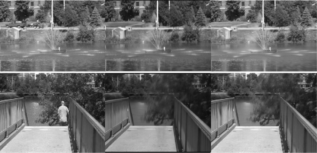
In order to evaluate the performance of the EM-RPCA, dynamic background sequences from CDnet and I2R dataset are used. As an example, Figure 5 shows the low-rank, foreground mask and dynamic background components recovered by EM-RPCA. We compare our results to the RPCA and TVRPCA (Cao et al. 2016). TVRPCA generalizes RPCA for the dynamic background cases by decomposing the sparse component from the RPCA model into changing background and specially connected foreground. The EM-RPCA enforces the connectivity of the foreground based on the overlaying model. Table 4 shows the F-measures for different video sequences. TVRPCA and EM-RPCA perform similarly in terms of this measure.

Table 4: Comparison of EM-RPCA with different methods on dynamic background.
EM-RPCA TVRPCA RPCA
WaterSurface 0.88 0.88 0.41
Fountain 0.81 0.80 0.57
Campus 0.77 0.77 0.72
Fountain 2 0.71 0.72 0.43
Overpass 0.78 0.77 0.46

Visual results in Fig. 4 and Fig. 7 on the other hand show that overlaying model is better capable of recovering the background in case where the foreground stops moving. The ROC curve and the histogram of the W\mathchar 29015 are shown in Fig. 6. The ROC curve shows slight improvement in terms of area under the curve. Additional visual results for another sequence are shown in Figures 8 and 9.

Refer to caption

Figure 5: Different components by EM-RPCA form left to right: Original frame, low-rank component L\mathchar 29004, foreground mask W\mathchar 29015, and dynamic changes of background E\mathchar 28997.

Refer to caption

Figure 6: (left) ROC curve for the result of different methods on WaterSurface data. (right) Histogram of the recovered W\mathchar 29015 from EM-RPCA.

Refer to caption

Figure 7: Visual results for the mask and the low-rank background for the slow moving sequence.

Refer to caption

Figure 8: Visual results for the mask for Fountain2(top row) and Overpass(bottom row) datasets from CDnet. Images form left to right: Original frame, Ground truth mask, EM-RPCA mask, TVRPCA mask, and RPCA mask.

Refer to caption

Figure 9: Visual results for the low-rank image for Fountain2(top row) and Overpass(bottom row) datasets from CDnet. Images form left to right: Original frame, low-rank component for EM-RPCA, and low-rank component for TVRPCA.

5 Conclusion

In this study, we introduced an extension of sparse and low-rank decomposition under overlaying model, and developed an optimization framework to solve it. We also propose an extension of our M-RPCA framework for the dynamic background. We also provide an analysis of the model convergence under reasonable assumptions. We performed an extensive experimental studies evaluating our model on multiple videos from CDnet and I2R datasets, and show improvements for both static and dynamic background over RPCA and its extensions. As future work, we plan to extend this framework for various scenarios such as camera jitter.

References

  • Barnich & Droogenbroeck (2011) Barnich, O. and Droogenbroeck, M. V. Vibe: A universal background subtraction algorithm for video sequences. IEEE Transactions on Image Processing, 20(6):1709–1724, June 2011. ISSN 1057-7149. doi: 10.1109/TIP.2010.2101613.
  • Boyd et al. (2011) Boyd, S., Parikh, N., Chu, E., Peleato, B., Eckstein, J., et al. Distributed optimization and statistical learning via the alternating direction method of multipliers. Foundations and Trends in Machine learning, 3(1):1–122, 2011.
  • Candès et al. (2011) Candès, E. J., Li, X., Ma, Y., and Wright, J. Robust principal component analysis? Journal of the ACM (JACM), 58(3):11, 2011.
  • Cao et al. (2016) Cao, X., Yang, L., and Guo, X. Total variation regularized rpca for irregularly moving object detection under dynamic background. IEEE Transactions on Cybernetics, 46(4):1014–1027, April 2016. ISSN 2168-2267. doi: 10.1109/TCYB.2015.2419737.
  • Chen et al. (2012) Chen, C.-F., Wei, C.-P., and Wang, Y.-C. F. Low-rank matrix recovery with structural incoherence for robust face recognition. In Computer Vision and Pattern Recognition (CVPR), 2012 IEEE Conference on, pp. 2618–2625. IEEE, 2012.
  • Ebadi & Izquierdo (2016) Ebadi, S. E. and Izquierdo, E. Foreground segmentation via dynamic tree-structured sparse rpca. In European Conference on Computer Vision, pp. 314–329. Springer, 2016.
  • Feng et al. (2013) Feng, J., Xu, H., and Yan, S. Online robust pca via stochastic optimization. In Advances in Neural Information Processing Systems, pp. 404–412, 2013.
  • Gao et al. (2014) Gao, Z., Cheong, L.-F., and Wang, Y.-X. Block-sparse rpca for salient motion detection. IEEE transactions on pattern analysis and machine intelligence, 36(10):1975–1987, 2014.
  • Goldfarb (2018) Goldfarb, D. Admm for multiaffine constrained optimization. 2018.
  • Kafieh et al. (2015) Kafieh, R., Rabbani, H., and Selesnick, I. Three dimensional data-driven multi scale atomic representation of optical coherence tomography. IEEE transactions on medical imaging, 34(5):1042–1062, 2015.
  • Keshavan et al. (2010) Keshavan, R. H., Montanari, A., and Oh, S. Matrix completion from noisy entries. Journal of Machine Learning Research, 11(Jul):2057–2078, 2010.
  • Li et al. (2004) Li, L., Huang, W., Gu, I. Y.-H., and Tian, Q. Statistical modeling of complex backgrounds for foreground object detection. IEEE Transactions on Image Processing, 13(11):1459–1472, 2004.
  • Lin et al. (2011) Lin, Z., Liu, R., and Su, Z. Linearized alternating direction method with adaptive penalty for low-rank representation. In Shawe-Taylor, J., Zemel, R. S., Bartlett, P. L., Pereira, F., and Weinberger, K. Q. (eds.), Advances in Neural Information Processing Systems 24, pp. 612–620. Curran Associates, Inc., 2011.
  • Maddalena et al. (2008) Maddalena, L., Petrosino, A., et al. A self-organizing approach to background subtraction for visual surveillance applications. IEEE Transactions on Image Processing, 17(7):1168, 2008.
  • Minaee & Wang (2017) Minaee, S. and Wang, Y. Masked signal decomposition using subspace representation and its applications. arXiv preprint arXiv:1704.07711, 2017.
  • Ng et al. (2010) Ng, M. K., Weiss, P., and Yuan, X. Solving constrained total-variation image restoration and reconstruction problems via alternating direction methods. SIAM journal on Scientific Computing, 32(5):2710–2736, 2010.
  • Peng et al. (2012) Peng, Y., Ganesh, A., Wright, J., Xu, W., and Ma, Y. Rasl: Robust alignment by sparse and low-rank decomposition for linearly correlated images. IEEE Transactions on Pattern Analysis and Machine Intelligence, 34(11):2233–2246, 2012.
  • Pope et al. (2011) Pope, G., Baumann, M., Studer, C., and Durisi, G. Real-time principal component pursuit. In Signals, Systems and Computers (ASILOMAR), 2011 Conference Record of the Forty Fifth Asilomar Conference on, pp. 1433–1437. IEEE, 2011.
  • Recht et al. (2010) Recht, B., Fazel, M., and Parrilo, P. A. Guaranteed minimum-rank solutions of linear matrix equations via nuclear norm minimization. SIAM review, 52(3):471–501, 2010.
  • Rockafellar & Wets (2009) Rockafellar, R. T. and Wets, R. J.-B. Variational analysis, volume 317. Springer Science & Business Media, 2009.
  • Wang et al. (2014) Wang, Y., Jodoin, P., Porikli, F., Konrad, J., Benezeth, Y., and Ishwar, P. Cdnet 2014: An expanded change detection benchmark dataset. In 2014 IEEE Conference on Computer Vision and Pattern Recognition Workshops, pp. 393–400, June 2014.
  • Yang & Yuan (2013) Yang, J. and Yuan, X. Linearized augmented lagrangian and alternating direction methods for nuclear norm minimization. Mathematics of computation, 82(281):301–329, 2013.
  • Yazdi & Bouwmans (2018) Yazdi, M. and Bouwmans, T. New trends on moving object detection in video images captured by a moving camera: A survey. Computer Science Review, 28:157–177, 2018.
  • Ye et al. (2015) Ye, X., Yang, J., Sun, X., Li, K., Hou, C., and Wang, Y. Foreground–background separation from video clips via motion-assisted matrix restoration. IEEE Transactions on Circuits and Systems for Video Technology, 25(11):1721–1734, Nov 2015.
  • Zhang et al. (2013) Zhang, Y., Jiang, Z., and Davis, L. S. Learning structured low-rank representations for image classification. In Proceedings of the IEEE Conference on Computer Vision and Pattern Recognition, pp. 676–683, 2013.
  • Zhang et al. (2012) Zhang, Z., Ganesh, A., Liang, X., and Ma, Y. Tilt: Transform invariant low-rank textures. International journal of computer vision, 99(1):1–24, 2012.
  • Zhao et al. (2012) Zhao, Z., Bouwmans, T., Zhang, X., and Fang, Y. A fuzzy background modeling approach for motion detection in dynamic backgrounds. In Multimedia and signal processing, pp. 177–185. Springer, 2012.
  • Zhou et al. (2013) Zhou, X., Yang, C., and Yu, W. Moving object detection by detecting contiguous outliers in the low-rank representation. IEEE Transactions on Pattern Analysis and Machine Intelligence, 35(3):597–610, March 2013.
  • Zivkovic (2004) Zivkovic, Z. Improved adaptive gaussian mixture model for background subtraction. In Pattern Recognition, 2004. ICPR 2004. Proceedings of the 17th International Conference on, volume 2, pp. 28–31. IEEE, 2004.