Dirichlet Depths for Point Process

It is well known that the point process can be equivalently represented by the inter-event times (IETs). Here the IETs of a point process $s_{1},s_{2},\cdots,s_{k}$ on $[T_{1},T_{2}]$ are given as $u_{1}=s_{1}-T_{1},u_{2}=s_{2}-s_{1},\cdots,u_{k}=s_{k}-s_{k-1},u_{k+1}=T_{2}-s_{k}$. The IET sequence $(u_{1},u_{2},\cdots,u_{k+1})$ has $k$ degrees of freedom and in fact forms a $k$-dimensional simplex (scaled standard simplex) as:

This simplex $X_{k}$ is bounded by the boundary set $B_{k}=\{u\in X_{k}:u_{i}=0\mbox{ for at least one }i\in\{1,2,\cdots,k+1\}\}.$ The points at boundary indicate a realization which has either two events happening simultaneously or one event happening at time $T_{1}$ or $T_{2}$. Both situations indicate extreme realizations (often with zero probability density) of a point process.

Based on this IET representation, we look for a conditional depth defined on the $X_{k}$ simplex. Notice that the normalized IET sequence $(\frac{u_{1}}{T_{2}-T_{1}},\frac{u_{2}}{T_{2}-T_{1}}$, $\cdots$, $\frac{u_{k+1}}{T_{2}-T_{1}})$ has the constant sum of 1. Therefore, one apparent option for the depth is the density function of Dirichlet distribution, which is commonly used as a prior in Bayesian statistics. Here we review the Dirichlet distribution which will be used to derive our conditional depth function: The Dirichlet probability density function of order $m\geq 2$ with concentration parameter vector $\mathbf{a}=(a_{1},a_{2},\cdots,a_{m})\in\mathbb{R}^{m}$ with $a_{i}>0$, $i=1,\cdots,m$, is given as:

where $(x_{1},x_{2},\cdots,x_{m})$ is in the standard $m-1$ simplex, i.e. $\sum_{i=1}^{m}x_{i}=1$ and $x_{i}\geq 0,i=1,2,\cdots,m$. This density function is denoted as $Dirichlet(\mathbf{a},m)$.

In statistical depth literature, Zuo & Serfling 2000a and Nieto-Reyes & Battey 2016 proposed important and desirable properties for depth on multivariate and functional data, respectively. They further claim that a depth function should be defined through desirable properties. Motivated by this claim, we list and discuss five desirable properties for a conditional depth function for point process as follow.

• •

  P-1, Continuity and vanishing at the boundary: Conditional depth for point process is a map from the simplex $X_{k}$ to $\mathbb{R}^{+}$. Since event times are continuous on the time domain, a minimal requirement for a proper conditional depth should be continuity. Also, an ideal conditional depth for point process should vanish at the boundary.

• •

  P-2, Maximality at the center: This may be the most logical one among all properties since the center must have a maximal depth in a center-outward rank. The notion of center can be defined using symmetric properties or the mathematical expectation.

• •

  P-3, Monotonicity relative to the deepest point: This property is also intuitive as depth value should decrease from the center in a center-outward trend.

• •

  P-4, Scale and shift invariance: The scale and shift invariance is a special case of the affine invariance in multivariate depth. Basically, a good depth is expected to be invariant with respect to scaling and translation on the time domain.

• •

  P-5, Time warping invariance: The variation of a point process must satisfy two conditions: 1) the events are in the domain $[T_{1},T_{2}]$, and 2) the events remain the temporal order. Such variation can be properly described by the set of time warping functions, defined as a boundary-preserving diffeomorphism $\Gamma=\{\gamma:[T_{1},T_{2}]\rightarrow[T_{1},T_{2}]\mid\gamma(T_{1})=T_{1},\gamma(T_{2})=T_{2},\dot{\gamma}>0\}$, where the dot indicates the first order derivative (Srivastava & Klassen 2016). The time warping essentially allows any order-preserving nonlinear transformation of events in the given time domain. The time warping invariance also corresponds to the affine invariance in multivariate depths.

In the following sections, we will discuss all above properties in proposed conditional depths.

For an HPP, the first term $w(|s|)$ in Equation (2.1) is simply the normalized Poisson probability on the number of events in the given process. The challenge therefore stays on the conditional depth $D_{c}(s\mid|s|)$. As we have discussed, defining conditional depth for HPP on its IET representation will address the natural order issue, and ideally, the conditional depth should satisfy Properties P-1 to P-4. Property P-5 is not applicable here since any non-linear time warping on an HPP will make the process not homogeneous anymore.

Before we step into the formal definition of Dirichlet depth, we first look at the connection between HPP and Dirichlet distribution. For an HPP, we have defined IETs $(u_{i}\ ,\ i=1,\cdots,k+1)$ as mentioned earlier. Conditioned on the number of events $k$, the normalized IETs $(\frac{u_{i}}{T_{2}-T_{1}}\ ,\ i=1,2,\cdots,k+1)$ will satisfy two conditions: (1) They share the same support, a $k$-dimensional standard simplex, as the Dirichlet distribution (also true for any point process). (2) They follow a flat $Dirichlet(\{1,\cdots,1\},k+1)$ distribution, which is in fact a uniform distribution over the standard $k$-dimensional simplex. The detail proof is given in Part A of the Supplementary Materials.

With a slight modification on Equation (2.2), we formally propose the Dirichlet depth for an HPP as follow:

The Dirichlet depth $D_{c}(s\mid|s|=k)$ for an HPP in Definition 2.2 describes the conditional depth of a realization when the number of events (cardinality) is known. In Equation (2.3), we have set the concentration parameters of the Dirichlet distribution $a_{i}$ as $1+\frac{1}{k+1}$ for $\ i=1,2,\cdots,k+1$. This constant value makes the Dirichlet depth a concave function with maximum at the conditional mean (the derivation is given in the next subsection). The scale constant $(k+1)$ ensures $D_{c}(s\mid|s|=k)$ has an onto map to $[0,1]$. This normalization makes conditional depths comparable for observations across different number of events.

When discussing the properties of a depth function on a given space (e.g. Dirichlet depth on a simplex), a central notion is the center which depends on the underlying probability distribution. In this paper, conditioned on $|s|=k$ we take the center as the common mathematical expectation. That is, the center is

Using the derivation in Part A of the Supplementary Materials, the center has the following closed-form:

Hence, the corresponding IET vector of conditional center is $(\frac{T_{2}-T_{1}}{k+1},\frac{T_{2}-T_{1}}{k+1}$, $\cdots,\frac{T_{2}-T_{1}}{k+1})$. On a $k$-dimensional simplex, this point is the same as the geometric center. For general point process other than the HPP, we will adopt the similar notion of center.

Now, we are ready to derive the important properties of the new conditional depth:

P-1, Continuity and vanishing at the boundary: $D_{c}(s\mid|s|=k)$ is a continuous map from $S_{k}$ to $[0,1]$. It is easy to verify that $D_{c}(s\mid|s|=k)=0$ if and only if the IET sequence of $s$ is in the boundary set $B_{k}$.

P-2, Maximality at the conditional mean (the center): Let $\theta_{k}=(\frac{T_{2}-T_{1}}{k+1},\frac{2(T_{2}-T_{1})}{k+1}$, $\cdots,$ $\frac{k(T_{2}-T_{1})}{k+1})$ denote the center of an HPP on $[T_{1},T_{2}]$ with cardinality $k$. Then $D_{c}(\theta_{k}\mid|\theta_{k}|=k)=\sup_{s\in S_{k}}D_{c}(s\mid|s|=k)=1$.

P-3, Monotonicity relative to the deepest point: For any $s\in S_{k}$ and $a\in[0,1]$, we can prove that $D_{c}(s\mid|s|=k)\leq D_{c}(\theta_{k}+a(s-\theta_{k})\mid|s|=k)$.

P-4, Scale and shift invariance: For any scaling coefficient $a\in\mathbb{R^{+}}$ and translation $b\in\mathbb{R}$, we define a transformation of $s$ as $s^{\prime}=as+b\textbf{1}$ (where $\textbf{1}=(1,1,\cdots,1)\in\mathbb{R}^{k}$). Let the time domain of $s$ be $[T_{1},T_{2}]$. Then the time domain of $s^{\prime}$ will be $[aT_{1}+b,aT_{2}+b]$. If we include the time domain in the definition of Dirichlet depth, then we can show that $D_{c}(s\mid|s|=k,T_{1},T_{2})=D_{c}(s^{\prime}\mid|s^{\prime}|=k,aT_{1}+b,aT_{2}+b)$.

The proofs of all these properties are given in Part B of the Supplementary Materials.

In this subsection, we will at first examine the ranking performance of the Dirichlet depth on $S_{2}$. We will then utilize the Dirichlet depth as the conditional depth in Equation 2.1 to study the ranking performance on 100 HPP realizations.

Conditioned on the cardinality $|s|=2$, the inter-event times are uniformly distributed on a 2-dimensional simplex. Here we simulate $100$ realizations from HPP conditional on $|s|=2$ in time interval $[0,1]$, and then apply both Dirichlet Depth for HPP (Equation 2.3) and Mahalanobis depth for comparison. The result is shown in Figure 2. We can see that compared with the (truncated) elliptic contours by the Mahalanobis depth, Dirichlet depth has smooth, triangle-like contours that are more compatible with the triangular IET domain. Also, the Mahalanobis depth assigns positive depth values for the points on the boundary, which is not reasonable in practice.

Next, we will apply Dirichlet depth for HPP (Equation (2.3)) as the conditional depth of the proposed depth framework (Equation (2.1)) on $100$ HPP realizations in interval $[0,10]$. The detailed procedure is: (1) Randomly generate $100$ HPP realizations in interval $[0,10]$ with intensity rate $\lambda=0.4$ (the expected number of events should be $4$). (2) Fit cardinality $|s|$ of sampled realizations into a Poisson model base on maximum Likelihood estimate of $\lambda$. Then use this model to compute probabilities $P(|s|=k)$ and normalize it as the first probability term $w(|s|=k)$ in Equation (2.1). (3) Apply the Dirichlet depth for HPP as the conditional depth of Equation (2.1) to compute depth value of each realization. The result is shown in Figure 3.

We can see that the depth values depend on both the probability term $w(|s|)$ and the conditional depth term, and the ranks vary with different choice of $r$. The deepest realization is the one with the largest weight ($|s|=4$) and evenly distributed (close to the center). When the value of $r$ changes from 1 to 10, the first term $w(|s|)$ becomes more dominant, so that realizations with cardinality close to $4$ are more likely to be ranked on the top. Note that $r$ is a hyperparameter in the depth definition. In practice, one can adjust $r$ to balance the probability term and the conditional depth term for different purposes. Alternatively, a cross-validation procedure may be applied to find an optimal value.

Defining Dirichlet depth for general point process is more challenging since there is no direct connection between Dirichlet distribution and point process (other than the HPP). In this paper, we propose two different approaches for the definition: (1) naturally extend Equation (2.3) to general point process, and (2) transform the process to an HPP and then adopt Equation (2.3). At first, we extend the Dirichlet depth in Equation (2.3) to a general point process in $[T_{1},T_{2}]$ by defining the center of IETs as the conditional mean of the process. The formal definition is given as follows.

For an HPP $s$ in $[T_{1},T_{2}]$ conditioned on cardinality $|s|=k$, we have showed that its conditional mean is: $(\frac{T_{2}-T_{1}}{k+1},\frac{2(T_{2}-T_{1})}{k+1},\cdots,\frac{k(T_{2}-T_{1})}{k+1})$. In this case, it is easy to verify that Equation (2.4) is simplified to Equation (2.3). Therefore, Dirichlet depth for HPP is a special case of Equation (2.4). Note that the conditional depth value in Equation (2.4) only depends on the conditional expectation of the process with the same cardinality, which can be estimated by the conditional sample mean given a collection of realizations. Hence, the sample version of Dirichlet depth can be obtained by replacing its conditional means with sample means. That is, we can write the sample Dirichlet depth as:

where $\overline{s}_{k}^{(n)}=(\overline{s}_{1,k}^{(n)},\overline{s}_{2,k}^{(n)},\cdots,\overline{s}_{k,k}^{(n)})$ are the estimated sample means conditioned on the cardinality $k$ of $n$ observed realizations.

For point processes in general, we also adopt the center as the conditional mean given cardinality $|s|=k$. That is, $\theta_{k}=\mathbb{E}(s\mid|s|=k)$. We can show that the Dirichlet depth of Equation (2.4) assigns the highest depth value $1$ to this center. For HPP, this center is always $(\frac{T_{2}-T_{1}}{k+1},\frac{2(T_{2}-T_{1})}{k+1},\cdots,\frac{k(T_{2}-T_{1})}{k+1})$, regardless of the constant intensity rate $\lambda$. However, in general, there is no closed-form expression of the conditional mean if the conditional intensity of the process is unknown. Indeed, we can prove that Properties P-1 to P-4 are satisfied by the general Dirichlet depth in Equation (2.4). The detailed proof is omitted due to its similarity to the HPP case.

Now we examine the time invariance property. Let $p=(p_{1}$, $\cdots,p_{k})$ be a random point process realization with $k$ events. Then the conditional mean is $\mathbb{E}(p\mid|p|=k)=(\mathbb{E}(p_{1}\mid|p|=k),\cdots,\mathbb{E}(p_{k}\mid|p|=k))$. Under time warping $\gamma\in\Gamma$, a point process $s=(s_{1},\cdots,s_{k})$ will become $\gamma(s)=(\gamma(s_{1})$, $\cdots,\gamma(s_{k}))$. Similarly, the conditional means will become $\mathbb{E}(\gamma(p)\mid|p|=k)=(\mathbb{E}(\gamma(p_{1})\mid|p|=k),\cdots,\mathbb{E}(\gamma(p_{k})\mid|p|=k)).$ To simplify the notation on the conditional means, we let $\mu_{i,k}=\mathbb{E}(p_{i}\mid|p|=k)$ and $\mu_{i,k,\gamma}=\mathbb{E}(\gamma(p_{i})\mid|p|=k),i=1,\cdots,k$ and $\mu_{0,k}=\mu_{0,k,\gamma}=T_{1},\mu_{k+1,k}=\mu_{k+1,k,\gamma}=T_{2}.$ If we include the conditional means in the definition, the Dirichlet depth on the transformed point process is:

The inequality holds because the time warping in general is a nonlinear transformation. That is, Property P-5 does not hold for the Dirichlet depth in Definition 2.3.

Dirichlet depth in Equation (2.4) relies heavily on the conditional means. For point process in general, there are no closed-forms for the conditional means if conditional intensity function is unknown. In practice, given a set of point process realizations, we can apply the sample version Equation (2.5) to estimate the Dirichlet depth. However, for a given training data set, the sample size usually is not sufficiently large to result in a proper estimation of the conditional mean for each cardinality $|s|$. Here we propose a bootstrapping approach to address this issue.

Given a data set of point process realizations $p_{1},p_{2},\cdots,p_{n}$, where $p_{i}$ is a vector in $\mathbb{R}^{|p_{i}|}$ for $i=1,2,\cdots,n$. In general, those vectors do not have the same dimension, and therefore it is not possible to take an average to compute the conditional sample mean as we need in sample Dirichlet depth. To address this issue, we propose a bootstrap method to resample each realization $p_{i}$ such that the resampled realizations $p^{\prime}_{i}$ has the desired dimension $k$. Then we can effectively estimate the conditional sample mean given cardinality $|s|=k$ by simply taking an average. The detailed steps are listed in Algorithm 1 as follows.

Note that we have defined the depth for HPP. For any point process, if we can find a way to transform it to an HPP, then the notion of Dirichlet depth can be directly applied. Actually, such transformation can be done using the well-known time re-scaling theorem (Brown et al. 2001). Basically, the theorem states that any point process with an integrable conditional intensity function can be converted into an HPP (Papangelou 1972; Karr 1991): Let $T_{1}<s_{1}<s_{2}<\cdots<s_{k}\leq T_{2}$ be a realization from a point process with a conditional intensity function $\lambda(t|H_{t})>0$ for all $t\in(T_{1},T_{2}].$ Then, the sequence $\Lambda(s_{i})=\int_{T_{1}}^{s_{i}}\lambda(t|H_{t})dt,i=1,\cdots,k$ is a Poisson Process with the unit rate in $(0,\Lambda(T_{2})]$.

By applying this theorem, the notion of Dirichlet depth can be extended to general point processes. For a point process with known conditional intensity function, we can apply the time re-scaling theorem to convert it into an HPP in $[0,1]$, and then use Equation (2.3) to compute its Dirichlet depth. Here we propose an alternative definition of the Dirichlet depth, referred to as time-rescaling-based (or TS-based) Dirichlet depth, as follows:

We can verify that the sequence $(\frac{\Lambda(s_{1})}{\Lambda(T_{2})},\cdots,\frac{\Lambda(s_{k})}{\Lambda(T_{2})})$ follows an HPP in $[0,1]$ with intensity $\Lambda(T_{2})$. For point processes without history dependence such as an inhomogeneous Poisson process (IPP), the re-scaled HPP realization will be distributed in a fix time interval $[0,\Lambda(T_{2})]$. However, for point processes with history dependence, the re-scaled HPP realizations have different time length. A normalization to the interval $[0,1]$ by dividing $\Lambda(T_{2})$ will help make comparison across realizations. Note that Definition 2.4 is not IET-based with respect to the original point process, and therefore there is no notion of simplex. This is fundamentally different from Definitions 2.2 and 2.3. Moreover, for an HPP in $[T_{1},T_{2}]$ with constant rate $\lambda$, $\Lambda(t)=\lambda(t-T_{1})$. Then Equation (2.6) is simplified to

Therefore, the TS-based Dirichlet depth also generalizes Definition 2.2 for HPP.

We examine the 5 properties of the time re-scaling based Dirichlet depth $D_{c-TS}$ (Equation 2.6). We will show that P-1, P-4, and P-5 still hold.

P-1: Continuity and vanishing at the boundary: The detailed proof of P-1 is shown in Part C of the Supplementary Materials.

P-2: Maximality at the center: The function $\Lambda(\cdot)$ varies with respect to each point process. Hence, in general, there could be multiple maxima in the TS-based Dirichlet depth and a unique center will not exist. However, in the special case of IPP, $\Lambda$ is a deterministic function for all processes. Let $\theta_{k}=(\frac{\Lambda(T_{2})}{k+1},\frac{2\Lambda(T_{2})}{k+1},\cdots,\frac{k\Lambda(T_{2})}{k+1})$ denote the center of an HPP on $[0,\Lambda(T_{2})]$ with cardinality $k$. It is easy to see that $D_{c-TS}(\Lambda^{-1}(\theta_{k})\mid|\theta_{k}|=k)=\sup_{s\in S_{k}}D_{c-TS}(s\mid|s|=k)=1$, and this center $\Lambda^{-1}(\theta_{k})$ is unique.

P-3: Monotonicity relative to the deepest point: As the center may not be unique, the monotonicity cannot hold.

P-4: Scale and shift invariance: The proof is similar to the one in the HPP case.

P-5, Time warping invariance: Under time warping $\gamma\in\Gamma$, a point process $s=(s_{1},s_{2},\cdots,s_{k})$ will become $\gamma(s)=(\gamma(s_{1}),\gamma(s_{2})$, $\cdots,\gamma(s_{k}))$. Similarly, we find that the transformed cumulative conditional intensity function $\Lambda_{\gamma}=\Lambda\circ\gamma^{-1}$. If we include the cumulative conditional intensity function in the definition of Dirichlet depth, we have

The detailed proof is given in Part D of the Supplementary Materials.

Comparing two different methods (Definitions 2.4 and 2.3) of defining Dirichlet depth for general point process, Definition 2.3 seems easier to apply in practice. If the conditional intensity function is known, the proposed TS-based definition is expected to have an effective center-outward ranking. However, the conditional intensity function is often unknown, particularly in practical use. In fact, perhaps the most challenging part of the TS-based Dirichlet depth in Equation (2.6) is to properly estimate the conditional intensity.

As a summary, we list the properties in the three Dirichlet depths (in Definitions 2.2, 2.3, and 2.4) in Table 1, where “T” denotes “true” and “F” denotes “false”.

In this subsection, we demonstrate the proposed Dirichlet depths using a simulated inhomogeneous Poisson process (IPP). We randomly generate $100$ IPP realizations on $[0,2\pi]$ with intensity function $\lambda(t)=1-cos(t)$. The generated realizations are shown in Figure 4(a). The total intensity is $\Lambda=\int_{0}^{2\pi}\lambda(t)dt=2\pi$, and therefore the probability of cardinality $P(|s|)$ reaches its maximum at $|s|=6$.

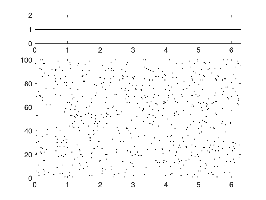
Given a sample set of a point process, we need to estimate the conditional means in order to apply sample Dirichlet depth and need to estimate the intensity function for TS-based Dirichlet depth. In this example, we use Algorithm 1 to estimate the conditional means. The intensity function of an IPP can be easily estimated with training samples.

We will also need to estimate the probability $P(|s|)$ in order to compute the first probability term $w(|s|)$ in Equation (2.1). In this illustration, $P(|s|)$ is estimated by the MLE algorithm based on Poisson distribution and remains the same under different depth functions. Moreover, the weight parameter $r$ is introduced to balance the importance of the first probability term and conditional depth. For illustrative purposes, we set $r$ to two different values of 1 and 0.01. The ranking result is shown in Figure 4.

Comparing Panels (b) and (e) (where $r=1$), we can see that the ranking results based on sample Dirichlet depth function and TS-based Dirichlet depth function are very similar – four out of five top-ranked realizations are the same. Similarly, four out of five bottom-ranked realizations are the same as well. We also compare Panels (c) and (f) where $r=0.01$. Although the overall ranks changed dramatically from where $r=1$, both methods agree on the four out of five deepest realizations, and four out of five shallowest realizations.

We have seen that both Dirichlet depths can identify the most ”typical” realizations whose distributions closely resemble the true intensity function. In order to illustrate the relationship between the Dirichlet depth and the goodness-of-fit, we treat each realization as a set of i.i.d. sampling points from the density function $f(t)=\frac{\lambda(t)}{\Lambda(2\pi)}$, and plot its P-values from the Kolmogorov-Smirnov (KS) test vs. its conditional Dirichlet depths in Figure 5.

We can see that both sample Dirichlet depth and TS-based Dirichlet depth are positively associated with the P-value of the KS test. This indicates more typical realizations correspond to larger Dirichlet depth values. Therefore, the proposed Dirichlet depths provide an alternative measurement for the “goodness-of-fit” of the given observations on the intensity function.

References

- (1)
- Barnett (1976) Barnett, V. (1976), ‘The ordering of multivariate data’, Journal of the Royal Statistical Society. Series A (General) 139(3), 318–355.
- Brown et al. (2001) Brown, E. N., Barbieri, R., Ventura, V., Kass, R. E. & Frank, L. M. (2001), ‘The time-rescaling theorem and its application to neural spike train data analysis’, Neural Computation 14, 325–346.
- Chen et al. (2009) Chen, Y., Dang, X., Peng, H. & Bart, H. L. J. (2009), ‘Outlier detection with the kernelized spatial depth function’, IEEE Transactions on Pattern Analysis and Machine Intelligence 31(2), 288–305.
- Dyckerhoff (2016) Dyckerhoff, R. (2016), ‘Convergence of depths and depth-trimmed regions’.
- Fraiman et al. (1999) Fraiman, R., Meloche, J., García-Escudero, L., Gordaliza, A., He, X., Maronna, R., Yohai, V., Sheather, S., Mckean, J., G. Small, C. & Wood, A. (1999), ‘Multivariate l-estimation’, Test 8, 255–317.
- Karr (1991) Karr, A. (1991), Point processes and their statistical inference, Second Edition,, Probability: Pure and Applied, Taylor & Francis.
- Koshevoy & Mosler (1997) Koshevoy, G. & Mosler, K. (1997), ‘Zonoid trimming for multivariate distributions’, Ann. Statist. 25(5), 1998–2017.
- Lange et al. (2014) Lange, T., Mosler, K. & Mozharovskyi, P. (2014), ‘Fast nonparametric classification based on data depth’, Statistical Papers 55(1), 49–69.
- Lawhern et al. (2011) Lawhern, V., A. A, N., Wu, W. & Contrares, R. J. (2011), ‘Spike rate and spike timing contributions to coding taste quality information in rat periphery’, Frontiers in Integrative Neuroscience 5, 1–14.
- Liu (1990) Liu, R. (1990), ‘On a notion of data depth based on random simplices’, The Annals of Statistics 18(1), 405–414.
- Liu et al. (1999) Liu, R. Y., Parelius, J. M. & Singh, K. (1999), ‘Multivariate analysis by data depth: descriptive statistics, graphics and inference, (with discussion and a rejoinder by liu and singh)’, Ann. Statist. 27(3), 783–858.
- Liu & Singh (1993) Liu, R. Y. & Singh, K. (1993), ‘A quality index based on data depth and multivariate rank tests’, Journal of the American Statistical Association 88, 252–260.
- Liu & Wu (2017) Liu, S. & Wu, W. (2017), ‘Generalized mahalanobis depth in point process and its application in neural coding’, Ann. Appl. Stat. 11(2), 992–1010.
- Lopez-Pintado & Romo (2009) Lopez-Pintado, S. & Romo, J. (2009), ‘On the concept of depth for functional data’, Journal of American Statistical Association 104(486), 718–734.
- Massé (2004) Massé, J.-C. (2004), ‘Asymptotics for the tukey depth process, with an application to a multivariate trimmed mean’, Bernoulli 10(3), 397–419.
- Mosler & Polyakova (2012) Mosler, K. & Polyakova, Y. (2012), ‘General notions of depth for functional data’, Manuscript 1981.
- Nieto-Reyes & Battey (2016) Nieto-Reyes, A. & Battey, H. (2016), ‘A topologically valid definition of depth for functional data’, Statist. Sci. 31(1), 61–79.
- Nolan (1992) Nolan, D. (1992), ‘Asymptotics for multivariate trimming’, Stochastic Processes and their Applications 42, 157–169.
- Oja (1983) Oja, H. (1983), ‘Descriptive statistics for multivariate distributions’, Statistics & Probability Letters 1(6), 327–332.
- Papangelou (1972) Papangelou, F. (1972), ‘Integrability of expected increments of point processes and a related random change of scale’, Transactions of the American Mathematical Society - TRANS AMER MATH SOC 165.
- Srivastava & Klassen (2016) Srivastava, A. & Klassen, E. P. (2016), Functional and Shape Data Analysis, Springer-Verlag New York.
- Tukey (1975) Tukey, J. W. (1975), ‘Mathematics and picturing data’, International Congress of Mathematicians 2, 523–531.
- Wu & Srivastava (2013) Wu, W. & Srivastava, A. (2013), ‘Estimating summary statistics in the spike-train space’, Journal of Computational Neuroscience 34, 391–410.
- Zuo & Serfling (2000a) Zuo, Y. & Serfling, R. (2000a), ‘General notions of statistical depth function’, Ann. Statist. 28(2), 461–482.
- Zuo & Serfling (2000b) Zuo, Y. & Serfling, R. (2000b), ‘Structural properties and convergence results for contours of sample statistical depth functions’, Ann. Statist. 28(2), 483–499.