Bayesian calibration and sensitivity analysis of heat transfer models for fire insulation panels
Abstract
A common approach to assess the performance of fire insulation panels
is the component additive method (CAM). The parameters of the CAM are based on
the temperature-dependent thermal material properties of the panels. These
material properties can be derived by calibrating finite element heat transfer
models using experimentally measured temperature records. In the past, the
calibration of the material properties was done manually by trial and error
approaches, which was inefficient and prone to error.
In this contribution, the calibration problem is reformulated in a
probabilistic setting and solved using the Bayesian model calibration
framework. This not only gives a set of best-fit parameters but also
confidence bounds on the latter. To make this framework feasible, the
procedure is accelerated through the use of advanced surrogate modelling
techniques: polynomial chaos expansions combined with principal component
analysis. This surrogate modelling technique additionally allows one to
conduct a variance-based sensitivity analysis at no additional cost by
giving access to the Sobol’ indices. The calibration is finally validated
by using the calibrated material properties to predict the temperature
development in different experimental setups.
Keywords: Bayesian model calibration, sensitivity analysis, surrogate modelling, component additive method, polynomial chaos expansions.
1 Introduction
Knowledge about the basic behaviour of materials exposed to fire is extremely important to successfully develop fire safety strategies. Depending on the type and height of buildings, certain fire requirements need to be fulfilled, e.g. requirements w.r.t. the load-bearing function (R) and separating function (EI). In case of timber buildings, the performance not only of the timber members, but also of protective materials such as gypsum plasterboards and insulations is of high importance for the fire design of the building structure. These different materials are usually combined to build floor and wall elements with different layups, so-called timber frame assemblies. The separating function of timber frame assemblies is usually verified using the component additive method (CAM) (Frangi et al. 2010; Mäger et al. 2017; Just and Schmid 2018). This method is rather flexible for calculating the separating function because it handles arbitrary layups made of various materials and thickness. Producers of fire protection products (e.g. gypsum plasterboard and insulation) need to determine input factors for the individual materials so that the separating function of a timber frame assembly with these materials can be verified using the CAM.
Indeed, the same protective material (e.g. a gypsum plasterboard with a given thickness) contributes differently to the fire resistance of a timber frame assembly in different setups. The CAM therefore considers (1) the material and thickness of a layer and (2) modification factors taking into account the neighbouring layers. This leads to a high number of possible combinations for timber frame assemblies, which cannot all be tested in fire resistance tests. Therefore, the factors of the CAM are usually derived based on finite element (FE) models and accompanying fire resistance tests.
Fire resistance tests using the standard EN/ISO temperature time curve according to ISO 834-1:1999 1999 and EN 1363-1:2012 2012 constitute the basis for these simulations. In the fire tests, the temperature is recorded over time inside the specimen at specific distances to the fire exposed surface. These recordings are used as a reference for FE simulations of the same setup. Heat transfer models using effective thermal material properties that depend on the temperature (specific heat capacity , thermal conductivity and material density ) are usually employed to simulate the temperature development inside timber frame assemblies exposed to fire. These material properties are then calibrated such that the output matches the recorded temperatures. Since these properties are not strictly physical quantities, they are called effective material properties. They account for not explicitly modeled effects such as fissures, cracks and moisture flow inside the specimen (Frangi et al. 2010). Despite these simplifications, using temperature-dependent effective material properties together with a common heat transfer analysis is appropriate and state-of-the-art for the calibration of parameters in the CAM. This is especially true since the introduced simplifications are negligible compared to the simplifications made within the CAM.
The conventional process of determining these effective material properties is slow and inaccurate as the calibration is usually done manually. All temperature measurements are averaged, thus eliminating the variability in the material behaviour and not accounting for it in the calibration. The derivation of thermal material properties is conventionally done as follows (Mäger et al. 2017):
- Step 1
Assume effective thermal material properties and simulate a specific layup with FE heat transfer models;
- Step 2
Compare the resulting temperatures with the averaged measurements;
- Step 3
A more rigorous calibration of these effective material properties can be achieved by parameterizing the thermal time-dependent material properties with a set of model parameters. Through this parametrization the problem of determining the time-dependent effective material properties is recast as a problem of determining the real-valued parameterizing model parameters. Then the calibration problem can be posed in a probabilistic setting. This allows a proper treatment of uncertainties arising from material fluctuations, measurement errors and model insufficiencies. One general way to do this is the so-called Bayesian inversion framework (Beck and Katafygiotis 1998; Gelman et al. 2014; Yu et al. 2019). In this framework, the model parameters are seen as random variables. Instead of trying to determine one particular value for these parameters, this probabilistic framework determines the full probability distribution of the model parameters conditioned on the observed measurements. This distribution contains much more information about the calibrated properties than the single point estimate from the conventional approach. For example, it allows computing expected values, maximum a posteriori estimates, confidence intervals on the calibrated values and the full correlation structure. Furthermore, the calibration can be verified easily by computing the posterior predictive distribution (Gelman et al. 1996).
To determine the probability distribution of the material properties, it is necessary to repeatedly evaluate the FE heat transfer model. To reduce the computational burden associated with repeated model evaluations, it has become customary to replace the computational forward model with a cheap-to-evaluate surrogate. Therefore, the Bayesian inversion framework is here combined with the polynomial chaos expansions (PCE) surrogate modelling technique (Sudret 2007; Blatman 2009; Guo et al. 2018).
When working with models with multiple input parameters, the question of the relative importance of individual parameters with respect to the output arises naturally. Quantifying this influence is called sensitivity analysis. One family of approaches are the so-called variance decomposition techniques (Saltelli et al. 2000; Arwade et al. 2010). These methods attempt to apportion the variance of the probabilistic model output to the individual input parameters. The Sobol’ indices are one such variance decomposition technique (Sobol’ 1993). Determining the Sobol’ indices is typically computationally expensive, but it has been shown by Sudret 2006 that they can be computed easily for a PCE surrogate model. Their computation allows valuable insights into the heat-transfer model’s properties.
In this paper, the material properties of four different gypsum insulation boards (Products A-D, E1-E4) are calibrated based on fire resistance tests carried out with these materials. These experimental results are presented and discussed in detail in Section 2. The calibration is carried out with the Bayesian model calibration framework accelerated by constructing a PCE-based surrogate model as detailed in Section 3. Section 4 outlines how the employed surrogate model can be used to conduct a global sensitivity analysis of the considered computational model. Finally, in Section 5, the calibration is verified using two fire tests that use two of the calibrated materials (Product C and Product D) in different experimental setups (V1 and V2).
2 Experiments and modelling
2.1 Experiments
Two fire resistance tests with horizontally oriented specimens constitute the experimental basis for the analysis in this paper (Just 2016; Breu 2016). The unloaded tests were conducted on the model-scale furnace of SP Wood Building Technology (today’s Research Institute of Sweden, RISE) and were exposed to the EN/ISO temperature-time curve (EN 1363-1:2012 2012; ISO 834-1:1999 1999). Two (V1 and V2, (Breu 2016)), respectively four (E1 to E4, (Just 2016)) different gypsum plasterboard setups with dimensions of were tested in each test (Figure 1). Tables 1 and 2 show the layups of the specimens. The space between and around the specimens was at least 100 mm and was filled with Product D boards to protect the carrying layer, i.e. the last layer. The carrying layer was a 19 mm particle board with density kg/m3 in Test 1 (specimens E1 to E4) and a Product D 15 mm in Test 2 (specimens V1 and V2). Figure 2 shows the specimens of Test 2 during fabrication.
In specimens E1 to E4 (Test 1), five wire thermocouples and one copper disc thermocouple measured the temperatures at a single interface between the layers. The fluctuations of the sensor readings can mainly be attributed to variations in the material properties. The measured temperatures are displayed in Figures to .
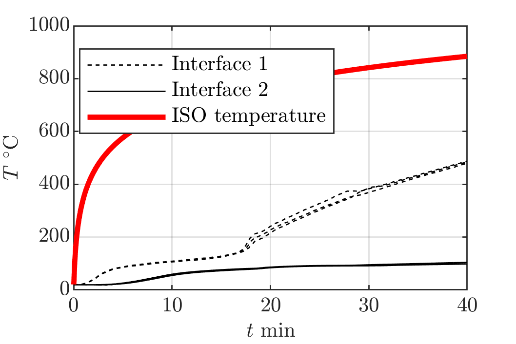
In specimens V1 and V2 (Test 2), three wire thermocouples were placed between each layer. The measured temperatures at the two interfaces 1 and 2 are displayed in Figures and .
Test 1 and Test 2, with specimens E1-E4 and V1,V2 respectively, were exposed to the EN/ISO standard temperature-time curve (EN 1363-1:2012 2012; ISO 834-1:1999 1999).
The temperature measurements at each sensor were collected at discrete time steps :
| (1) |
where and . For simplicity, the superscript is omitted unless required to distinguish between individual measurements. Therefore, in the sequel stands for a vector of measurements captured by a single sensor.
| Layer 1 | Layer 2 | |||
|---|---|---|---|---|
| E1 | Product A | 12.5 mm | particle board | 19 mm |
| E2 | Product B | 9.5 mm | particle board | 19 mm |
| E3 | Product C | 12.5 mm | particle board | 19 mm |
| E4 | Product D | 15 mm | particle board | 19 mm |
| Layer 1 | Layer 2+3 | |||
|---|---|---|---|---|
| V1 | Product C | 12.5 mm | Product D | 215 mm |
| V2 | Product D | 15 mm | Product D | 215 mm |


1: exposed protection layer, Product C; 2: protection layer Product D; 3: carrying layer Product D; around the specimen other protection layers were applied to protect the carrying layer.



2.2 Forward modelling
The experiments described in the previous section were modeled using one-dimensional heat transfer FE-models. The reduction to a one-dimensional setup is justified, because it is known that the experimental heat-flux is mostly perpendicular to the exposed surface. The simulations were conducted using the general purpose finite element software Abaqus (Abaqus FEA 2017). The energy input on the heated surface and the losses on the unexposed side took into account the energy input/loss through convection and radiation.
The radiation temperature was assumed to be equal to the gas temperature and followed the EN/ISO temperature-time curve EN 1363-1:2012 2012; ISO 834-1:1999 1999 on the exposed side and was constantly on the unexposed side (as in the experiments). The emissivity was taken as and the convection coefficient as according to EN 1991-1-2:2002 2002. The element size in the FE-mesh was . The temperature-dependent material properties of the particle board (Test 1) were taken from Schleifer 2009.
The unknown parameters of interest are the temperature-dependent effective material properties of the insulation material: the thermal conductivity , the heat capacity and the material density of the investigated insulation materials.
With this, the computational forward model is
| (2) |
For every set of material properties, this model returns the temperature evolution at locations and at times where measurements are available (see Section 2.1).
Since each of those parameters is a function of the temperature, they cannot be directly calibrated. Instead, these functions have to be parameterized with a set of scalar parameters, as described next.
2.3 Parametrization of material properties
The parametrization of the three temperature-dependent material properties () is a crucial step of the calibration procedure. It consists of specifying a set of parameters that define the shape of the temperature-dependent function that describes each material property. The choice of these parameters is delicate, as it imposes a certain temperature-dependent behaviour on the material properties. A priori, there are no physical constraints on this thermal behaviour besides positivity, so generally, the properties are defined as , and .
One further complication lies in the fact that these properties are mere effective properties and cannot generally be measured. To find constraints on these parameters, it is thus necessary to rely on previous calibration attempts of gypsum insulation boards (Breu 2016; Schleifer 2009) in conjunction with measurements of certain properties, where available.
By gathering information from such previous attempts, the thermal properties are parameterized by six parameters . This parametrization is flexible enough to enable inference on and follows physical and empirical reasoning as described next.
We propose to distinguish two key processes during which the temperature-dependent material properties change significantly:
- First key process
-
When the free water content in the gypsum insulation boards evaporates, the latent water content of gypsum, which is composed of sulfate dihydrate CaSO4 2 H2O, evaporates. In this process, evaporation first forms calcium sulfate hemihydrate CaSO4 1/2 H2O (also called bassanite) and then anhydrate III CaSO4. The evaporation consumes heat, which is modelled as a local increase of the specific heat capacity, a reduction in the conductivity and a reduction in the material density.
- Second key process
-
Thermogravimetric analyses have shown a second peak in the specific heat due to chemical metamorphosis at elevated temperatures of secondary components found in the gypsum insulation boards (Schleifer 2009). This second key process is modelled as an increase in the material conductivity, a peak in the specific heat and a further reduction of the material density.
The temperatures at which these two key processes occur cannot be equally well prescribed a priori. While the temperature of the water evaporation is well known to occur at approximately with its main effect taking place at until it tails off at , the second key process cannot be characterized this precisely. It is assumed that the second key process starts at the unknown temperature and ends at . Additionally, the relative location of its main effect between and is parameterized with . These two temperatures heavily influence the evolution of the thermal properties and are thus used as temperatures of change in all effective material properties.
In the present setting of heated gypsum boards, the initial conductivity at ambient temperature is assumed to be (Breu 2016). During the first key process, the conductivity is assumed to linearly decrease to a second value that is parameterized by . Starting with the second key process the conductivity starts to increase linearly to another value that is parameterized by , reached at the highest simulation temperature of .
Phase changes require a significant amount of energy. To model the energy requirement associated with the evaporation of water trapped inside the insulation material, the specific heat is modelled with two piecewise linear spikes during both key processes, while being constant at (Schleifer 2009) for the other temperatures. The specific heat at the peaks is parameterized by for the first process and for the second one.
During the first and second key process, gaseous products are emitted (water and carbon dioxide respectively) and thus the density of the gypsum reduces. This density reduction was studied in Schleifer 2009 and the results are applied here directly. Starting from the density measured at room temperature , linearly reduces during the first key process to . It then remains constant and linearly reduces further to from the start of the second key process to the main effect of the second key process. The parametrization of the material properties is visualized in Figure 4.


To finalize the parametrization, reasonable ranges are defined for all parameters. These ranges correspond to bounds on the parameters that are the results of prior calibration attempts along with expert judgement. These ranges are given along with a summary of the parameters in Table 3 with plots of the resulting temperature-dependent material properties in Figure 5.
These six parameters are gathered into a vector , which fully characterizes the temperature-dependent behaviour of the gypsum insulation boards.
| Parameter | Physical Meaning | Range | Unit |
|---|---|---|---|
| Start of second key process | |||
| Main effect of second key process | - | ||
| (relative between and ) | |||
| and | |||


2.4 Finite element model
The FE model is considered as a verified simulator for the transient heat propagation in gypsum insulation panels under fire exposure. This means that the model is assumed to accurately solve the underlying differential equations posed by the mathematical heat transfer model. For a review of techniques for rigorous model verification see Oberkampf et al. 2004; Oberkampf and Roy 2010.
The FE model yields a discretized time-dependent temperature curve for each realization of the parameter vector that parameterizes the effective thermal properties , and . The discretization of the time steps is identical to the available measurements, so that with .
3 Model calibration
The process of finding model parameters so that the model evaluation using this parameter vector agrees with some observations is called calibration. A general probabilistic framework for calibration is presented next. For simplicity, it is assumed that only one measurement series is available for now. This restriction is lifted in Section 5.
3.1 The Bayesian calibration approach
All models are simplifications of reality and all observations made in the real world contain measurement errors. To explicitly account for this combined mismatch between model output and observations, one option is to model the discrepancy as an additive mismatch between the model predictions and the observations:
| (3) |
One way to address the calibration problem of determining is to formulate it in a probabilistic setting. The unknown model discrepancy from Eq. (3) is then seen as a random vector. Commonly and in this work, is assumed to follow a zero mean normal distribution with a covariance matrix parameterized by a set of parameters :
| (4) |
Additionally, in the probabilistic setting, the combined parameter vector is assumed to be distributed according to a so-called prior distribution (to be further specified)
| (5) |
Then the discrepancy distribution from Eq. (4) can be used together with Eq. (3) to construct a model giving the probability of the observations given a realization of the parameter vector. Denoting by a realization of , this probability as a function of the parameters is the so-called likelihood function
| (6) |
which reads more explicitly:
| (7) |
With these definitions, it becomes possible to apply the Bayes’ theorem for conditional probabilities (Gelman et al. 2014):
| (8) |
where is the prior distribution of the input parameters , is the posterior distribution and is a normalizing factor called evidence.
The probability distributions in this expression can be interpreted as degrees of belief about the parameters (Beck and Katafygiotis 1998). Low values of the distribution at a realization indicate low confidence in this particular value, whereas high values indicate high confidence. With this interpretation of probabilities, Eq. (8) encodes the shift of belief about the parameter vector from before to after the observation of experiments . This process is called Bayesian updating, Bayesian inference or Bayesian inversion.
As mentioned above, the probability distributions in Bayes’ theorem are named according to their information content about the parameters in the setting of the updating procedure:
- Prior distribution :
-
this distribution captures the belief about the parameters before (i.e. prior to) observing data. In the setting of Bayesian updating for model calibration, it is chosen according to expert opinion and possible prior calibration attempts. A typical choice is to select a reasonable, although sufficiently large range (lower/upper bounds) for each parameter.
- Posterior distribution :
-
the posterior distribution is the conditional distribution of the parameters given the observations. It can be regarded as the state of information about the parameters after (i.e. to) making observations.
Thus, the computation of the posterior distribution can be considered as the solution of the calibration problem. Since it is a probability distribution rather than a single value, it encompasses all information specified by the prior distribution and the newly observed data. Already conceptually it is thus a much broader way of defining calibration than single value estimators.
Another probability distribution of interest in the Bayesian inference setting is the posterior predictive distribution . It is defined as
| (9) |
This distribution expresses beliefs about future (i.e. predictive) observations given the already observed ones . If it is possible to sample from the posterior distribution, i.e. , a sample from the posterior predictive distribution is obtained by drawing
| (10) |
The posterior predictive distribution allows to assess the predictive capabilities of the model following calibration. It contains the uncertainty about the model parameters and the mismatch parameters . Because this distribution is defined in the space where the data are collected, it can be used to visually check the calibration results.
3.2 Sampling from the posterior distribution
The analytical computation of the posterior distribution is typically not possible. This is mostly due to difficulties in evaluating the normalizing constant defined in Eq. (8). Its computation typically relies on estimating an integral in the parameter space, which is in most cases intractable.
A breakthrough technique called Markov chain Monte Carlo (MCMC) sampling, originally developed by Metropolis et al. 1953 and Hastings 1970, completely avoids the need to evaluate this high-dimensional integral. It is a type of stochastic simulation technique that constructs Markov chains that are guaranteed to produce samples distributed according to the posterior distribution. Posterior characteristics (e.g. quantities of interest, expected values, marginal distributions etc.) can then be estimated using this sample.
Following the initial development of the MH algorithm (Metropolis et al. 1953; Hastings 1970), recent developments to improve the algorithm’s efficiency strived towards adaptive proposal distributions (Haario et al. 2001; Roberts and Rosenthal 2009) and the utilization of gradient information (Rossky et al. 1978; MacKay 2003). One common flaw of these algorithms, however, is the requirement to tune them using a set of tuning parameters. This is a particularly tedious task that is a major source of error in practical applications.
The affine-invariant ensemble sampler (AIES, (Goodman and Weare 2010)) is a fairly recent MCMC algorithm that performs particulary well in this respect. This algorithm requires only a single tuning parameter and its performance is invariant to affine transformations of the target distribution. This property makes it particularly useful for real-world applications, where strong correlations between individual parameters often hinder conventional MCMC algorithms.
The AIES algorithm relies on a set of parallel chains where proposal samples are obtained by moving in the direction of a randomly chosen conjugate sample from a different chain. The pseudo-code for the implementation used in this paper is given in Algorithm 1.
A property that makes MCMC algorithms especially suitable for Bayesian computations is that they do not require the explicit computation of the normalization constant (from Eq. (8)), as only a posterior ratio, called acceptance ratio, is required (Step 9 of Algorithm 1). In this ratio, cancels out. However, the computationally expensive forward model must be evaluated each time this acceptance ratio is computed. This necessity of many runs of computationally expensive models has spurred the idea of constructing a surrogate model that, after successful construction, can be used in the MCMC algorithms in lieu of the original model, whereby the overall computational burden is reduced to feasible levels.
3.3 Surrogate modelling of the temperature time series
Often, sampling based techniques (e.g. MCMC algorithms) are considered infeasible because of the high number of computationally expensive model runs required. Surrogate modelling techniques try to solve this problem by constructing a computationally cheap emulator that can be used instead of the original model.
Non-intrusive approaches to construct surrogate models are solely based on realizations of the model parameters and corresponding model outputs (Choi et al. 2004). The set of parameters used for constructing the surrogate is referred to as experimental design, which means here a set of computer experiments and shall no be confused with physical experiments. Following the assembly of the experimental design, the constructed surrogate model aims to approximate the original model predictions denoted by ,
| (11) |
This section details the construction of a surrogate model combining polynomial chaos expansions (PCE) with the principal component analysis (PCA).
3.3.1 Polynomial Chaos Expansions
Polynomial chaos expansions (PCE) are a surrogate modelling technique that has been used extensively in the engineering disciplines (Xiu and Karniadakis 2002; Soize and Ghanem 2004; Guo et al. 2018) to construct surrogate models of scalar-valued functions of random variables. A brief introduction to the method is presented next.
Assume a random vector with mutually independent components . Its joint probability density function is thus given by
| (12) |
The functional inner product of two polynomials of degree and respectively, is then defined by
| (13) |
By choosing these polynomials to fulfil , i.e. if and 0 otherwise, these polynomials form a family of univariate orthonormal polynomials . There exist well-known families of polynomial functions that fulfil the fundamental condition of Eq. (13) w.r.t. standard parametric probability distributions (Askey and Wilson 1985).
These univariate polynomials can be used to build multivariate polynomials by tensor product. Introducing the multi-indices the latter are defined by:
| (14) |
It can be shown that the univariate orthonormality property of Eq. (13) extends to the multivariate case and that the following holds:
| (15) |
These polynomials form a so-called orthonormal basis of the space of square integrable functions with respect to the probability distribution . Any such function can be represented by:
| (16) |
where are the coefficients of the expansion.
In practical applications it is not feasible to compute the infinite number of coefficients . Instead, a truncation scheme is typically proposed that reduces the number of considered polynomials to a finite set. This truncated set denoted by transforms the equality of Eq. (16) to an approximation
| (17) |
In regression-based approaches, the coefficient vector is typically estimated by least-squares analysis, as originally proposed in Berveiller et al. 2006. This corresponds to selecting a truncation set (Blatman and Sudret 2011a) and using an experimental design to minimize the expression
| (18) |
By storing the function evaluations at in a vector the solution of Eq. (18) reads:
| (19) |
where are the evaluations of the basis polynomials on the experimental design .
To assess the accuracy of the obtained polynomial chaos expansion, the so-called generalization error shall be evaluated. A robust error measure can be obtained by using the leave-one-out (LOO) cross validation technique. This estimator is obtained by
| (20) |
where is constructed by leaving out the -th point from the experimental design. After some algebraic manipulation, it can be shown that the LOO error can be computed as a mere post-processing of the PCE expansion as follows
| (21) |
where is the component of the vector given by:
| (22) |
for more details refer to Blatman and Sudret 2010.
This section outlined the approach to use PCE for approximating scalar quantities. Since the heat transfer model considered in this paper returns a vector of interface temperatures at time steps, a pure PCE approach would require the construction of independent polynomial chaos expansions. Instead, a dimensionality reduction technique on the output is applied before using the PCE technique.
3.3.2 Principal Component Analysis
Because the discretized temperature evolution is expected to be rather smooth (see Figure 11), considerable correlation between the individual time steps is expected. This correlation can be exploited to reduce the dimensionality of the output in the context of surrogate modelling.
There exist numerous so-called dimensionality reduction techniques (van der Maaten et al. 2008), one of which is principal component analysis (PCA, Jolliffe 2002). The latter utilizes an orthogonal transformation to express in a new basis of uncorrelated principal components .
In practice, PCA is carried out by computing estimators of the expectation and the covariance matrix . The eigenvectors of this covariance matrix are denoted by for . The associated eigenvalue corresponds to the variance of in direction of the -th principal component. Thereby the random vector can be expressed through its principal components as .
The model output can then be compressed to a lower dimensional subspace by retaining only those principal components with the highest variance:
| (23) |
The number of terms is selected such that , with typically chosen as . This way, the model output can be approximated by a linear transformation of the principal component vector thereby reducing the problem dimensionality from to .
3.3.3 Combining PCA with PCE
The combination of PCA with PCE gives rise to an efficient surrogate modelling technique as shown originally in Blatman and Sudret 2011b. Constructing polynomial chaos expansions of each retained principal component , together with the PCA formulation from Eq. (23) yields a surrogate model relating the model parameters to the vector valued time series output of the transient heat transfer problem:
| (24) |
which can be rewritten by introducing the union set :
| (25) |
For compactness, this equation can also be expressed in matrix form by letting be a matrix containing the retained eigenvectors . For the PCE part of the equation the vector is introduced that holds the individual multivariate orthogonal polynomials. Let be a matrix that stores the corresponding PCE coefficients, then Eq. (24) can be written as
| (26) |
For completeness, the response can also be expressed for each random variable individually. For this, the row vector , taken from the -th row of the matrix of eigenvectors , is introduced:
| (27) |
This surrogate model can then be used in lieu of the original computationally expensive forward model. The evaluation of the surrogate model is orders of magnitude faster than the original finite element model. For comparison, in our application example a single FE run takes about on a conventional computer, while in the same time evaluations of the surrogate model can be made.
This reduction in computational time is a promising feature of the presented surrogate modelling technique. It does, however, come at the cost of a series of approximations that are introduced during the PCA and PCE computation. To ensure confidence in the produced surrogate model, a general error measure has to be devised. It includes the approximation error due to the PCA truncation and the truncated polynomial chaos expansion. Such an error measure was derived in Blatman and Sudret 2013. For the sake of completeness the details are given in A.
3.4 Summary of the proposed method
In this section, a procedure to efficiently conduct Bayesian inference with expensive vector valued models was presented. It is assumed that the parametrization of the temperature-dependent effective material properties (see Section 2.3) is known. Bayesian inference then aims at determining the distribution of the parameters after observations (i.e. experimental measurements) have been made. A brief step-by-step account of this procedure is given below for reference:
- Step 1
Choose a prior distribution on and construct an experimental design using samples from this prior. Evaluate the forward model at and store the evaluations in .
- Step 2
Approximate using the surrogate model from Eq. (26). This requires the combination of the dimensionality reduction technique PCA with the PCE uncertainty propagation technique.
- Step 3
- Step 4
Define a likelihood function from Eq. (7) that captures the discrepancy between a model run and the observations.
- Step 5
Run the AIES defined in Algorithm 1 where the likelihood function uses the surrogate model instead of the original model to obtain a sample from the posterior distribution .
- Step 6
This method works if the support domain of the prior distribution contains that of the posterior distribution. In this respect, sufficiently large prior ranges shall be selected based on the expert’s judgment.
The successful calibration of the parameters through the Bayesian inference approach gives insight into the model mismatch and correlation structure between individual parameters. The distribution of the parameters can further be used in probabilistic analysis using these models and, given new observations, can be updated to reflect beliefs incorporating the newly acquired information.
A fundamental ingredient of the presented approach is the necessity to define a parametrization of the thermal effective material properties as described in Section 2.3. To judge the quality of the parametrization, it can be helpful to assess the relative importance of a single model parameter with respect to the output. For this, it is necessary to resort to the field of sensitivity analysis.
4 Sensitivity analysis
4.1 PCE based Sobol’ indices
Global sensitivity analysis aims at finding which input parameters of a computer model (or combination thereof) explain at best the uncertainties in the model predictions. In this respect, variance decomposition techniques rely on assigning fractions of the model output variance to the individual input parameters . For simplicity, in this section the subscript from the parameter vector is dropped.
Consider a scalar-valued computational model , which maps a vector of input parameters in the unit hypercube to the real numbers. This computational model can be decomposed into a sum of terms that only depend on a subset of the input parameters, i.e. a constant , univariate functions , bivariate functions etc.
| (28) |
This decomposition is called the Hoeffding-Sobol’ decomposition and is unique for any function that is square-integrable over the unit hypercube (Sobol’ 1993).
Denoting by a subset of indices, Eq. (28) can be written in short:
| (29) |
It can be shown that the terms of this equation called summands, are orthogonal (Sobol’ 1993). The variance of each term , called partial variance, is obtained by:
| (30) |
Due to the orthogonality of the terms in this equation, the total variance of the model output is finally obtained as the sum of the partial variances
| (31) |
Each partial variance describes the amount of the output variance that can be attributed to the interaction of the input variables . In particular, describes the fraction of the variance that can be attributed to one input variable taken separately.
Moreover, the total contribution to the variance attributable to a single input parameter is captured in the sum of the partial variances that contain the -th input variable. The sum of these partial variances normalized by the total variance is called the -th total Sobol’ index and is defined as
| (32) |
It is noted here that the sum of all total Sobol’ indices, i.e., , is larger than one because the same interaction effect contributes to multiple total Sobol’ indices. Usually the integral in Eq. (30) can be computed through Monte Carlo integration. However, if the model is expressed in an orthogonal basis (as is the case for PCE, Eq. (16)), the Sobol’ indices can be computed analytically by post-processing the PCE coefficients (Sudret 2006; Sudret 2008):
| (33) |
i.e. is the set of multivariate polynomials that are non-constant in the -th input parameter . For scalar-valued models, this yields a measure of the variance fraction that can be attributed to a certain input parameter. In the following section, this concept is extended to models with multiple outputs.
4.2 PCA-based Sobol’ indices
In the present paper models with multiple outputs (i.e. time-series of computed temperatues) are considered. By using a surrogate model that combines PCE with PCA, as discussed in Section. 3.3.3, the total Sobol’ indices for each output vector component (i.e. time step) can also be computed analytically (Marelli and Sudret 2015; Nagel et al. 2020).
For this, the partial variances of the model response components are computed by using the expression from Eq. (27). The total Sobol’ index for the -th component of the output random vector then reads
| (34) |
where is the subset of for which . The interested reader is referred to B for the derivations.
5 Results
In this section, the procedure presented in Sections 3 and 4 is applied to calibrate the temperature-dependent material properties of gypsum based insulation boards. The experimental data stems from experiments conducted by Breu 2016 and Just 2016 that were presented in Section 2.1. As explained in Section 2.3, the material properties are parameterized with a set of parameters. In the Bayesian inference framework introduced in Section 3.1, determining the posterior distribution of these parameters constitutes the calibration of the temperature-dependent material properties.
To further investigate the effects of the introduced parametrization, the surrogate models used for calibration are reused to conduct time-dependent sensitivity analyses (Section 4). These analyses show the influence each model parameter has on the simulation output. They deliver valuable insights and can be used to further refine the model parametrization.
Finally, the calibrated time-dependent material properties are validated by simulating insulation panels in a different measurement setup and comparing these simulation results with actual measurements.
5.1 Calibration of material properties for gypsum boards
In this section the general calibration procedure from Section 3.4 is applied to the specific problem of calibrating heat transfer models describing the experiments of specimens E1-E4 (Test 1) presented in Section 2.1.
The model parameters are assumed to be priorly independent and uniformly distributed with the lower and upper bounds ( and respectively) defined by the ranges given in Table 3. The prior distribution of the model parameters is thus given by
| (35) |
Since multiple measurements are available for each experiment, the formulation for the likelihood Eq. (6) has to be slightly adapted. Under the assumption of independence between the individual measurement locations, it can be written as the product
| (36) |
which generalizes Eq. (6) where only a single time series of measurements was considered. Consequently, the posterior distribution obtained from Bayes’ theorem should strictly be written as , but for notational simplicity the superscript (s) is again dropped.
The covariance matrix is parametrized by
| (37) |
where we choose a so-called Matérn autocorrelation function ():
| (38) |
In this autocorrelation function, is the correlation length and is the standard deviation at the -th time step. To reduce the number of calibration parameters, it is assumed that the standard deviation follows a degree- polynomial function
| (39) |
where is the -th Legendre polynomial (defined over ) and are the coefficients to be calibrated. As a summary, there are parameters to define our discrepancy term, namely which define the non-stationary variance of the model discrepancy, and the autocorrelation length . Using the notation from Section 3.1, we pose . To complete the prior information, a uniform distribution is assumed for the discrepancy parameters with non-restrictive bounds. A summary of the full prior distribution is given in Table 4.
| c.o.v. | units | |||||
|---|---|---|---|---|---|---|
| - | ||||||
| - | ||||||
| - | ||||||
| s |
Figure 6 shows the resulting sample points of the posterior distribution obtained for an exemplary calibration run for the E1 setup. This sample was produced using the previously presented AIES algorithm (Algorithm 1).


Despite the broad information contained in the full posterior plot, one is often interested in the set of parameters that best describe the observations. In accordance with the Bayesian interpretation of probabilities, this parameter set is located at the maximum value of the posterior distribution (maximum a posteriori, MAP). It can be found by solving the optimization problem
| (40) |
This problem can be approximately solved by picking the parameter point from the available posterior sample that maximizes the unnormalized posterior distribution . The resulting maximum a posteriori estimator is also shown in Figure 6.
The calibrated posterior parameters for Product A (E1) are summarized in Table 5. It gives an overview of the calibrated parameters, including a set of summary statistics.
A major advantage full samples have compared to point estimators is that they allow investigating characteristics of the posterior distribution. This provides a fuller picture of the calibrated parameter vector,e.g. by showing dependence between individual parameters , allowing the computation of confidence intervals or revealing problems with identifiability.
Additionally, the full parameter distribution explains why it can be hard to calibrate with the conventional approach. When strong correlations exist, such as for and in Figure 6, it is hard to move to a better guess by changing just one parameter.
In conclusion, the reduction of the standard deviation in all posterior parameters in conjunction with the unimodal posterior distribution can be seen as an indicator of a successful calibration.
| MAP | conf. interval | c.o.v. | |||
|---|---|---|---|---|---|
5.2 Discussion of the calibration results
The results of the proposed calibration procedure for four different insulation materials are discussed next. The materials are all characterized by the temperature-dependent material properties . The calibration results for Product A are summarized in Figure 7 and Table 5. In C the results of the remaining products are presented. The discussion in this section refers to them at times. In this section we use the notation and to more clearly distinguish between the prior and posterior random variables.
For each material, Figures and show the temperature-dependent conductivity and heat capacity . Since the full posterior distribution of the parameters is inferred, the plots do not only show one line for prior and posterior, but samples each. The shown curves result from prior parameter draws (i.e. before calibration), posterior parameter draws (i.e. after calibration) and the MAP parameter (see Eq. (40)). The calibrated density is not shown, since its two governing parameters and can be seen also in the plots of the calibrated and . It is obvious that the posterior samples have a smaller variance than the prior samples since the bandwith of the curves is much smaller.
A plot of the model predictions together with the measured data is presented in Figures . These plots show runs of the surrogate model before calibration () and confidence intervals of the predictions of the surrogate model following calibration (see Eq. (9)). The MAP parameter is propagated through the surrogate and the response of the original finite element model for is also plotted. Additionally, samples from the posterior are used to show the calibrated discrepancy standard deviation (see Eq. (39)).
To emphasize the reduction in uncertainty by the presented calibration procedure, additionally posterior distributions of the predicted temperature at snapshot times and are shown in Figures and . These plots show kernel density estimates of the output probability density function of the surrogate model before calibration and after calibration at the respective times . Additionally, the measured data and the MAP predictions are displayed. These plots are now discussed in more detail.
The distributions of (conductivity between and the start of the second key process) and (distribution of the heat capacity at ), show a large variance reduction. This means that the information gained about these parameters through the conducted calibration is high.
Generally, it can be expected that the heat capacity and the conductivity correlate, since a higher heat flow due to a higher conductivity can be compensated by a higher heat capacity, resulting in the same temperature profile. This is indeed the case for the parameters and as well as for and (which describe the conductivity and the heat capacity at higher temperatures), as seen in Figure 6. The effect of this correlation and its compensation effect can be seen by comparing Figure 13 (E2) to Figures 7 (E1), 15 (E3) and 17 (E4). Despite the fact that parameters and show a higher posterior variance for specimens E1, E3 and E4 than for E2, the variance of the resulting model predictions (Figures ) is comparable.
Despite the fact that the shown prior thermal material properties in Figures and are based on the same prior assumptions for the parameters , the modes of the prior distributions estimated from are significantly different for the individual specimens. This is caused by two factors: (1) the variable layer thickness and (2) the parametrization. The layer thickness influences the measured temperature simply by the fact that the further inside the specimen the measurement is placed, the colder it is at a certain time. This can easily be seen by comparing the different Figures , from mm (Figure 13) to mm (Figures 7 and 15) to mm (Figure 17). Additionally, parameter , the start time of the second key process, is responsible for the large variance of the start time of the temperature increase after the plateau. For higher values of , the plateau is longer and the temperature increase starts later. Thus if the snapshots (Figures and ) are taken where most prior temperatures are still at the plateau, the probability density functions have positive (right) skew. The later the snapshot is drawn, the more negatively skewed is the probability density function and the larger its variance gets.
Product B (E2) is the only product where the conductivity decreases after 400°C and where there is hardly a second key process according to the posterior curves. This shows that this product is made of a significantly different material.
Generally, all posterior predictive distributions agree well with the measurements. This suggests that the used heat transfer model with the chosen parametrization is sufficiently accurate to reproduce the observations.
The calibrated temperature-dependent material properties show a higher variance reduction at lower temperatures. This is mostly due to the maximum system temperature at being only as seen in Figure 3.
It can be clearly seen in Figures that the calibrated discrepancy standard deviation varies similarly across all four experiments. It is influenced by two factors: (1) the temperature variance from the data series (i.e. the individual sensor recordings) and (2) model insufficiencies that hinder a fully accurate reproduction of the data. The latter can be reduced by changing the parametrization: an additional model parameter between approximately and could reduce the calibrated mismatch standard deviation for the temperature increase after the plateau. This temperature range currently lacks an independent parameter.


5.3 Time-dependent sensitivity analysis
Using the PCA+PCE surrogate model and the derivations from Section 4, the constructed surrogate model of the temperature evolution can be reused to compute the time-dependent Sobol’ indices as measures for the individual model parameters’ importance across the simulation time.
The time-dependent Sobol’ indices were computed for all four surrogate models constructed for the experimental setups E1-E4. They are displayed in Figures 8 for Product A. In C the results of the remaining products are presented. The discussion in this section refers to them at times.
Generally there is no single parameter that clearly dominates the simulation output across the whole simulation time range. Instead, most parameters have a clear time range where they are important and other time ranges where their influence can be neglected. All parameters show a similar behaviour across the four models.
At early simulation times before , the Sobol’ indices and clearly dominate the sensitivity analysis across all four models. These indices correspond to the parameters (low to mid temperature conductivity) and (specific heat capacity at ). This is not surprising, because the system temperature is monotonously increasing and low temperature effects like these are expected to have a higher impact at earlier times. The Sobol’ index carries on to influence the simulation at later times, while decreases in importance towards the end of the simulation.
Starting from , the Sobol’ indices , and become dominant. This can be explained similarly, since they influence the mid to high temperature behaviour. is the start of the second key process and thus heavily influences the high temperature behaviour of all temperature-dependent material properties. (high temperature conductivity) and (specific heat capacity at the second key process) are the high temperature material properties and as such are more important at later time steps of the simulation.
The second key process results in a temperature plateau (like the one at ). Because this process occurs at temperatures higher than the maximum temperature reached at the measurement location, the process has no direct effect there. The system does, however, reach higher temperatures at locations closer to the exposed surface and it is there that the second key process influences the system behaviour. As can be seen from the results of the sensitivity analysis, the magnitude of the second key process () significantly influences the temperatures at the measurement location due to the locally lower thermal diffusivity. However, the temperature where this peak in the thermal diffusivity appears (), is not so important.

5.4 Validation of the calibration using V1-V2
So far, all presented results were related to the experiments Test 1 (specimens E1-E4) described in Section 2.1. It was shown that the calibrated material properties for the examined materials can be used to conduct computer simulations that agree well with the same experimental observations that were used for calibration (Section 5.1). Before these calibrated material properties can be used to make predictions about the material behaviour in other experimental setups, validation experiments need to be carried out to judge the accuracy for the new intended use (Oberkampf and Roy 2010).
In this work, the results from Test 2 (specimens V1 and V2) are used for this purpose (see Figure and ). These tests were conducted using two of the materials for which calibrated material properties were obtained (Product C (E3) and Product D (E4)). To validate the calibration results, the posterior predictive distribution of this setup needs to be computed. It is defined identically to Eq. (9) and samples from it can be drawn by
| (41) |
where the subscripts and were introduced to distinguish between quantities and models belonging to the respective setups. In this sense, refers to the finite element model predicting the heat evolution in the two interfaces of Test 2 and are measurements from Test 1.
Using parameters calibrated in Test 1 for the predictions in Test 2 requires careful consideration of the implications. On the one hand, the model parameters of the insulation products can be reused without further considerations (since this is the point of the validation). On the other hand, parameters related to the discrepancy model cannot be transferred so easily.
The discrepancy term captures measurement noise and model inadequacy and is assumed to follow a zero mean normal distribution (Eq. (4)). It cannot be directly applied in drawing predictive quantities as neither the measurement noise nor the model inadequacy can be expected to be identical between the two setups. Therefore, simplifying assumptions about the discrepancy covariance matrix have to be made.
The only information available about the discrepancy covariance matrix are the calibration results of E1-E4 (Section 5.1). There it was parameterized as described in Eq. (37). Across all posterior parameter distributions, the MAP estimator of the correlation length parameter was . The discrepancy standard deviation , however, did not yield such a uniform result as can be clearly seen from Figures 13 to 17. To still parameterize the covariance matrix in the predictive draws from Eq. (41), a conservative choice of and a constant is thus made. This corresponds to setting the discrepancy parameter vector to
| (42) |
Figures 9 and 10 show the resulting confidence intervals from the posterior predictive distribution defined in Eq. (41) for interface 1 and 2 of Test 2. To show the agreement of the predictions with the measurements, are displayed as well. The figures contain one time-temperature plot in Figures and summary statistics of the model predictions in Figure at snapshot times and respectively.
Generally the simulations agree remarkably well with the experimental observations, but there are also time intervals, where small differences between the predicted and observed temperature evolutions are visible. The predictions at large time instants, which are of interest in practice, appear excellent.

| () | Interface 1 | Interface 2 | Interface 1 | Interface 2 |
|---|---|---|---|---|

| () | Interface 1 | Interface 2 | Interface 1 | Interface 2 |
|---|---|---|---|---|
6 Summary and conclusion
In this paper, a procedure to calibrate temperature-dependent effective material properties of fire insulation panels was presented. Available experimental temperature measurements were modelled using a 1D finite element heat transfer model. Because the associated material properties vary with temperature, they were parameterized using a set of model parameters. The actual calibration was then carried out using the well-known Bayesian inference framework. The necessary sampling from the posterior distribution was conducted with the advanced AIES (Affine invariant ensemble sampler) MCMC algorithm. In an effort to reduce the computational burden from the required repeated finite element simulations, a surrogate model of the heat transfer problem was constructed by combining polynomial chaos expansions (PCE) with the principal component analysis (PCA) technique. This surrogate model offered the possibility to additionally conduct a sensitivity analysis using the time-dependent Sobol’ indices at no additional computational cost. Finally, the calibration was validated using a secondary set of experiments.
The proposed approach is superior to the previously used brute-force calibration approach because it automates the process, clearly defines the discrepancy and explicitly considers the uncertainties present in the model and measurements. Accordingly, it does not only deliver a single best fit property, but returns the full multivariate distribution of the calibrated properties and allows the computation of confidence intervals. Furthermore, the used Bayesian framework is a natural way to update information through the use of conditional random variables. It is well suited for engineering problems, where often expert knowledge is available that thereby can be directly integrated into the calibration procedure. However, it needs to be considered that depending on the application less general calibration procedures might be more suitable (Mottershead et al. 2011; Patelli et al. 2017).
A valuable side product of the presented surrogate modelling technique is the free computation of the time-dependent Sobol’ indices. This sensitivity analysis offers valuable insight into the time-dependent effect of the used parametrization.
Finally, it is worth emphasizing that the proposed method, which combines surrogate modelling (PCE) with dimensionality reduction (PCA), an advanced MCMC algorithm (AIES) and global sensitivity analysis is general and can be applied to any calibration problem involving complex computer codes. All the algorithms used are available in the UQLab uncertainty quantification software (Marelli and Sudret 2014), especially the recently developed Bayesian inversion module (Wagner et al. 2019).
Acknowledgement
The authors gratefully acknowledge the European COST Action FP1404 on the fire safe use of bio-based building products. Additionally, we would like to thank Prof. Alar Just and his team, as well as Dr. Joseph Nagel, who participated in the preliminary discussions about the case study definitions. The PhD thesis of the first author is supported by ETH grant #44 17-1.
Appendix A Surrogate model approximation error
The following approximation error was originally derived in Blatman and Sudret 2013. The surrogate model from Eq. (26) has a total -approximation error that can be written by denoting the -norm as by
| (43) | ||||
| (44) |
Through the Cauchy-Schwarz inequality this error is bounded by
| (45) | ||||
| (46) |
- PCA error :
-
this incorporates the error from estimating the mean and covariance matrix of the response as well as the dimensionality reduction error from leaving out dimensions. The former is neglected in this paper and for the latter the sum of the discarded eigenvalues can be directly used:
(47) - PCE error :
-
this is the error of the polynomial chaos approximation. It can be estimated as the sum of the individual LOO errors for the scalar-valued principal component PCE’s:
(48)
For practicality a relative error measure is preferred. This can be obtained by dividing the estimator of the absolute error bound by an estimator of , such as the trace of its estimated covariance matrix :
| (49) |


Figure 11 shows the resulting error estimate for a set of experimental designs and included principal components using the setup E1. Additionally, the actual and surrogate model are run for a set of parameters and plotted for comparison.
Appendix B Derivation of PCA-based Sobol’ indices
This appendix contains the derivations for PCA-based Sobol’ indices. To simplify the derivations, we introduce the notation to denote the random vector that contains all but the -th random variable . In the following derivations, the subscript in the expectation and variance operators and denotes the variable(s) with respect to which expectation and variance are computed, i.e. .
The total Sobol’ index for the -th element of a vector valued model output is defined as
| (50) |
This can be used to write an expression for the variance of the expectation of the -th model output as
| (51) | ||||
| (52) |
By introducing the expression for the surrogate model from Eq. (27) and the fact that the expectation of the -th response is , the following is obtained:
| (53) | ||||
| (54) | ||||
| (55) | ||||
Because the expectation of all principal components vanishes (), one can write
| (56) |
By switching to the summation notation, this can also be written as
| (57) |
Because the inner sum is only over the coefficients , this can be further simplified by substituting to obtain:
| (58) | ||||
| (59) | ||||
| (60) |
Due to the orthonormality of the polynomial basis , the conditional expectation in this equation can be expressed analytically as
| (61) |
Therefore, the variance of the conditional expectation from Eq. (50) becomes
| (62) |
where is the subset that contains only those polynomials with . For completeness the total variance in the denominator of Eq. (50) reads:
| (63) |
The total PCA-based index for the -th component of the output vector is thus obtained by plugging these results into Eq. (50):
| (64) |
Appendix C Additional results
This section presents the calibration and sensitivity analysis results for Product B, Product C and Product D.
| MAP | conf. interval | c.o.v. | |||
|---|---|---|---|---|---|


| MAP | conf. interval | c.o.v. | |||
|---|---|---|---|---|---|


| MAP | conf. interval | c.o.v. | |||
|---|---|---|---|---|---|


References
- Abaqus FEA (2017) Dassault Systèmes (Ed.) (2017). ABAQUS/Standard User’s Manual, Version 6.14.
- Arwade et al. (2010) Arwade, S. R., M. Moradi, and A. Louhghalam (2010). Variance decomposition and global sensitivity for structural systems. Engineering Structures 32(1), 1–10.
- Askey and Wilson (1985) Askey, R. and J. Wilson (1985). Some basic hypergeometric polynomials that generalize Jacobi polynomials. Memoirs of the American Mathematical Society 54(319), 1–57.
- Beck and Katafygiotis (1998) Beck, J. L. and L. S. Katafygiotis (1998). Updating models and their uncertainties. I: Bayesian statistical framework. Journal of Engineering Mechanics 124(4), 455–461.
- Berveiller et al. (2006) Berveiller, M., B. Sudret, and M. Lemaire (2006). Stochastic finite elements: a non intrusive approach by regression. European Journal of Computational Mechanics 15(1-3), 81–92.
- Blatman (2009) Blatman, G. (2009). Adaptive sparse polynomial chaos expansions for uncertainty propagation and sensitivity analysis. Ph. D. thesis, Université Blaise Pascal, Clermont-Ferrand.
- Blatman and Sudret (2010) Blatman, G. and B. Sudret (2010). An adaptive algorithm to build up sparse polynomial chaos expansions for stochastic finite element analysis. Probabilistic Engineering Mechanics 25, 183–197.
- Blatman and Sudret (2011a) Blatman, G. and B. Sudret (2011a). Adaptive sparse polynomial chaos expansion based on Least Angle Regression. Journal of Computational Physics 230, 2345–2367.
- Blatman and Sudret (2011b) Blatman, G. and B. Sudret (2011b). Principal component analysis and Least Angle Regression in spectral stochastic finite element analysis. In M. Faber, J. Köhler, and K. Nishijima (Eds.), Proceedings 11th International Conference on Applications of Statistics and Probability in Civil Engineering (ICASP11), Zurich, Switzerland.
- Blatman and Sudret (2013) Blatman, G. and B. Sudret (2013). Sparse polynomial chaos expansions of vector-valued response quantities. In G. Deodatis (Ed.), Proceedings 11th International Conference on Structural Safety and Reliability (ICOSSAR’2013), New York, USA.
- Breu (2016) Breu, R. D. (2016). Improved component additive method for the separating function - development of a testing and calculation procedure. Master’s thesis, ETH Zürich, Switzerland.
- Choi et al. (2004) Choi, S., R. Grandhi, R. Canfield, and C. Pettit (2004). Polynomial chaos expansion with Latin Hypercube sampling for estimating response variability. AIAA Journal 45, 1191–1198.
- EN 1363-1:2012 (2012) EN 1363-1:2012 (2012). Feuerwiderstandsprüfungen - Teil 1: Allgemeine Anforderungen. Technical report, Deutsches Institut für Normung, Berlin, DE.
- EN 1991-1-2:2002 (2002) EN 1991-1-2:2002 (2002). Eurocode 1: Actions on structures - Part 1-2: General actions - Actions on structures exposed to fire. Technical report, European Committee for Standardization, Brussels, BE.
- Frangi et al. (2010) Frangi, A., V. Schleifer, and M. Fontana (2010). Design model for the verification of the separating function of light timber frame assemblies. Engineering Structures 32(4), 1184–1195.
- Gelman et al. (2014) Gelman, A., J. B. Carlin, H. S. Stern, D. B. Dunson, A. Vehtari, and D. B. Rubin (2014). Bayesian Data Analysis (3 ed.). Texts in Statistical Science. CRC Press.
- Gelman et al. (1996) Gelman, A., X.-L. Meng, and H. Stern (1996). Posterior predictive assessment of model fitness via realized discrepancies. Statistica Sinica 6(4), 733–760.
- Goodman and Weare (2010) Goodman, J. and J. Weare (2010). Ensemble samplers with affine invariance. Communications in Applied Mathematics and Computational Science 5(1), 65–80.
- Guo et al. (2018) Guo, X., D. Dias, C. Carvajal, L. Peyras, and P. Breul (2018). Reliability analysis of embankment dam sliding stability using the sparse polynomial chaos expansion. Engineering Structures 174(1), 295–307.
- Haario et al. (2001) Haario, H., E. Saksman, and J. Tamminen (2001). An adaptive Metropolis algorithm. Bernoulli 7(2), 223–242.
- Hastings (1970) Hastings, W. K. (1970). Monte Carlo sampling methods using Markov chains and their applications. Biometrika 57(1), 97–109.
- ISO 834-1:1999 (1999) ISO 834-1:1999 (1999). Fire-resistance tests - Elements of building construction. Technical report, International Organization for Standardization, Geneva, CH.
- Jolliffe (2002) Jolliffe, I. T. (2002). Principal Component Analysis (2 ed.). Springer Series in Statistics. Springer-Verlag.
- Just (2016) Just, A. (2016). Model scale fire tests of four gypsum plasterboards of Gyproc and stone wool. Test report 5P08165-03, SP Technical Research Institute of Sweden.
- Just and Schmid (2018) Just, A. and J. Schmid (2018). Guidance for implementation of materials and products in fire design methods of timber frame assemblies. Technical report, COST Action FP1404, Zürich, Switzerland.
- MacKay (2003) MacKay, D. J. C. (2003). Information Theory, Inference and Learning Algorithms. Cambridge University Press.
- Mäger et al. (2017) Mäger, K. N., A. Just, J. Schmid, N. Werther, M. Klippel, D. Brandon, and A. Frangi (2017). Procedure for implementing new materials to the component additive method. Fire Safety Journal 107, 149–160.
- Marelli and Sudret (2014) Marelli, S. and B. Sudret (2014). UQLab: A framework for uncertainty quantification in Matlab. In Vulnerability, Uncertainty, and Risk (Proceedings 2nd International Conference on Vulnerability, Risk Analysis and Management (ICVRAM2014), Liverpool, United Kingdom), pp. 2554–2563.
- Marelli and Sudret (2015) Marelli, S. and B. Sudret (2015). Compressive polynomial chaos expansion for multi-dimensional model maps. In T. Haukaas (Ed.), Proceedings 12th International Conference on Applications of Statistics and Probability in Civil Engineering (ICASP12), Vancouver, Canada. Paper #209.
- Metropolis et al. (1953) Metropolis, N., A. W. Rosenbluth, M. N. Rosenbluth, A. H. Teller, and E. Teller (1953). Equation of state calculations by fast computing machines. The Journal of Chemical Physics 21(6), 1087–1092.
- Mottershead et al. (2011) Mottershead, J. E., M. Link, and M. I. Friswell (2011). The sensitivity method in finite element model updating: A tutorial. Mechanical Systems and Signal Processing 25(7), 2275–2296.
- Nagel et al. (2020) Nagel, J., J. Rieckermann, and B. Sudret (2020). Principal component analysis and sparse polynomial chaos expansions for global sensitivity analysis and model calibration: application to urban drainage simulation. Reliability Engineering & System Safety 195.
- Oberkampf and Roy (2010) Oberkampf, W. and C. Roy (2010). Verification and Validation in Scientific Computing. Cambridge University Press.
- Oberkampf et al. (2004) Oberkampf, W., T. Trucano, and C. Hirsch (2004). Verification, validation, and predictive capability in computational engineering and physics. Applied Mechanics Reviews 57(5), 345–384.
- Patelli et al. (2017) Patelli, E., Y. Govers, M. Broggi, H. Gomes, M. Link, and J. Mottershead (2017). Sensitivity or Bayesian model updating: a comparison of techniques using the DLR AIRMOD test data. Archive of Applied Mechanics 87, 905–925.
- Roberts and Rosenthal (2009) Roberts, G. O. and J. S. Rosenthal (2009). Examples of adaptive MCMC. Journal of Computational and Graphical Statistics 18(2), 349–367.
- Rossky et al. (1978) Rossky, P. J., J. D. Doll, and H. L. Friedmann (1978). Brownian dynamics as smart Monte Carlo simulation. The Journal of Chemical Physics 69(10), 4628–4633.
- Saltelli et al. (2000) Saltelli, A., K. Chan, and E. Scott (Eds.) (2000). Sensitivity analysis. J. Wiley & Sons.
- Schleifer (2009) Schleifer, V. (2009). Zum Verhalten von raumabschliessenden mehrschichtigen Holzbauteilen im Brandfall. Ph. D. thesis, ETH Zürich, Switzerland.
- Sobol’ (1993) Sobol’, I. (1993). Sensitivity estimates for nonlinear mathematical models. Mathematical Modeling & Computational Experiment 1, 407–414.
- Soize and Ghanem (2004) Soize, C. and R. Ghanem (2004). Physical systems with random uncertainties: chaos representations with arbitrary probability measure. SIAM Journal on Scientific Computing 26(2), 395–410.
- Sudret (2006) Sudret, B. (2006). Global sensitivity analysis using polynomial chaos expansions. In P. Spanos and G. Deodatis (Eds.), Proceedings 5th International Conference on Computational Stochastic Mechanics (CSM5), Rhodos, Greece.
- Sudret (2007) Sudret, B. (2007). Uncertainty propagation and sensitivity analysis in mechanical models – contributions to structural reliability and stochastic spectral methods. Technical report. Habilitation à diriger des recherches, Université Blaise Pascal, Clermont-Ferrand, France (229 pages).
- Sudret (2008) Sudret, B. (2008). Global sensitivity analysis using polynomial chaos expansions. Reliability Engineering & System Safety 93, 964–979.
- van der Maaten et al. (2008) van der Maaten, L., E. Postma, and H. van den Herik (2008). Dimensionality reduction: a comparative review. Journal of Machine Learning Research 10, 66–71.
- Wagner et al. (2019) Wagner, P.-R., J. Nagel, S. Marelli, and B. Sudret (2019). UQLab user manual – Bayesian inference for model calibration and inverse problems. Technical report, Chair of Risk, Safety & Uncertainty Quantification, ETH Zurich. Report # UQLab-V1.2-113.
- Xiu and Karniadakis (2002) Xiu, D. and G. Karniadakis (2002). The Wiener-Askey polynomial chaos for stochastic differential equations. SIAM Journal on Scientific Computing 24(2), 619–644.
- Yu et al. (2019) Yu, B., R. Tang, and B. Li (2019). Probabilistic calibration for development length models of deformed reinforcing bar. Engineering Structures 182(1), 279–289.