2-knot homology and Yoshikawa move

1. Introduction

Topological invariants of knots in ${\mathbb{R}}^{3}$ are constructed by Ng [11], [12], [13], [14], in a combinatorial method. These invariants are equivalent to the knot contact homology, constructed by Ekholm, Etnyre, Ng, Sullivan [3] in symplectic topology, and extended by Cieliebak, Ekholm, Latschev, Ng [2]. The knot contact homology detects several classes of knots [5], and an enhancement of the knot contact homology is a complete invariant of knots [4].

A surface-knot is a closed connected oriented surface embedded locally flatly in ${\mathbb{R}}^{4}$ . A surface-knot is represented by an oriented marked graph diagram, an oriented knot diagram equipped with 4-valent marked vertices [10], [16]. Extending Ng’s construction of knot invariants, we define in $\lx@sectionsign$ 2 a differential graded algebra $(CY(D),\partial)$ associated with an oriented marked graph diagram $D$ that represents a surface-knot in ${\mathbb{R}}^{4}$ .

Theorem 1.1.

Let $D_{0}$ , $D_{1}$ denote diagrams of an oriented marked graph representing a surface-knot in ${\mathbb{R}}^{4}$ . Then $(CY(D_{0}),\partial)$ is stably tame isomorphic to $(CY(D_{1}),\partial)$ .

Theorem 1.1 shows that the stably tame isomorphism class of $(CY(D),\partial)$ is an invariant of $F$ , where $D$ denotes a diagram of an oriented marked graph representing a surface-knot $F$ in ${\mathbb{R}}^{4}$ . Therefore the homology of $(CY(D),\partial)$ is an invariant of $F$ , which we denote by $HY(F)$ and call Yoshikawa homology. In $\lx@sectionsign\lx@sectionsign$ 3-11, we give a proof of Theorem 1.1. In $\lx@sectionsign$ 12, we show that the 0-dimensional homology $HY_{0}(F)$ distinguishes the spun-trefoil [1] from the 2-twist spun-trefoil [17].

Theorem 1.2.

Let $T^{0}(2,3)$ denote the spun-trefoil, and let $T^{2}(2,3)$ denote the 2-twist spun-trefoil in ${\mathbb{R}}^{4}$ . Then $HY_{0}(T^{0}(2,3))$ is not isomorphic to $HY_{0}(T^{2}(2,3))$ .

2. Definition

Let $G$ denote a finite regular graph with 4-valent vertices $v_{1},\cdots,v_{q}$ . We fix a rectangular neighborhood $V_{i}$ of $v_{i}$ which is homeomorphic to $\{(x,y)\in{\mathbb{R}}^{2}\ |\ -1\leq x\leq 1,-1\leq y\leq 1\}$ , where $v_{i}$ corresponds to the origin, and edges incident to $v_{i}$ in $V_{i}$ correspond to the subset $\{(x,y)\in{\mathbb{R}}^{2}\ |\ -1\leq x\leq 1,x^{2}=y^{2}\}$ . An interval given by $\{(x,0)\in{\mathbb{R}}^{2}\ |\ -1\leq x\leq 1\}$ on $V_{i}$ , called a marker, is attached to each $v_{i}$ . A marked graph is a spatial graph with markers in ${\mathbb{R}}^{3}$ . An orientation of a marked graph $G$ is a choice of an orientation on each edge of $G$ such that orientations on four edges near a marked vertex $v_{i}$ are chosen as one of the right two figures in Figure 1 for $i=1,\cdots,q$ . A marked graph is orientable if it admits an orientation. An oriented marked graph is an orientable marked graph with a fixed orientation. Two oriented marked graphs are equivalent if they are ambient isotopic in ${\mathbb{R}}^{3}$ keeping rectangular neighborhoods of marked vertices and orientations. A marked graph can be described by a diagram on ${\mathbb{R}}^{2}$ , which is a link diagram with 4-valent vertices equipped with markers. Given a marked graph diagram $D$ , let $L_{+}(D)$ (resp. $L_{-}(D)$ ) denote a link diagram obtained from $D$ by performing a resolution on a marked vertex $v_{i}$ along the marker (resp. along an arc perpendicular to the marker) in $V_{i}$ for $i=1,\cdots,q$ . See Figure 2. A marked graph diagram $D$ is admissible if both $L_{+}(D)$ and $L_{-}(D)$ represent trivial links. A marked graph is admissible if it has an admissible diagram.

Refer to caption — Figure 1. crossing (left) and marked vertex (center and right)

Let $p\colon{\mathbb{R}}^{4}\to{\mathbb{R}}$ denote a projection. We denote by ${\mathbb{R}}_{t}^{3}$ the hyperplane $p^{-1}(t)$ of ${\mathbb{R}}^{4}$ , where $t\in{\mathbb{R}}$ . A surface-link is a closed oriented surface embedded locally flatly in ${\mathbb{R}}^{4}$ . Kawauchi, Shibuya, Suzuki [7] showed that every surface-link ${\mathcal{L}}$ in ${\mathbb{R}}^{4}$ can be deformed by an ambient isotopy of ${\mathbb{R}}^{4}$ to a surface-link ${\mathcal{L}}^{\prime}$ , called a hyperbolic splitting of ${\mathcal{L}}$ , such that the projection $p|_{{\mathcal{L}}^{\prime}}\colon{\mathcal{L}}^{\prime}\to{\mathbb{R}}$ satisfies the following properties:
$(1)$ all critical points of $p|_{{\mathcal{L}}^{\prime}}$ are non-degenerate,
$(2)$ all the index 0 critical points (minimal points) of $p|_{{\mathcal{L}}^{\prime}}$ lie in ${\mathbb{R}}_{-1}^{3}$ ,
$(3)$ all the index 1 critical points (saddle points) of $p|_{{\mathcal{L}}^{\prime}}$ lie in ${\mathbb{R}}_{0}^{3}$ , and
$(4)$ all the index 2 critical points (maximal points) of $p|_{{\mathcal{L}}^{\prime}}$ lie in ${\mathbb{R}}_{1}^{3}$ .
The cross-section ${\mathcal{L}}^{\prime}\cap{\mathbb{R}}_{0}^{3}$ is a spatial 4-valent graph in ${\mathbb{R}}_{0}^{3}$ . We assign a marker to each 4-valent vertex (saddle point) so that the cross-section ${\mathcal{L}}^{\prime}\cap{\mathbb{R}}_{\varepsilon}^{3}$ (resp. ${\mathcal{L}}^{\prime}\cap{\mathbb{R}}_{-\varepsilon}^{3}$ ) is obtained from ${\mathcal{L}}^{\prime}\cap{\mathbb{R}}_{0}^{3}$ by performing a resolution along the marker (resp. along an arc perpendicular to the marker) at each vertex, where $\varepsilon$ is a small positive number. See Figure 2. The resulting spatial graph with markers in ${\mathbb{R}}_{0}^{3}$ is an admissible marked graph. A hyperbolic splitting ${\mathcal{L}}^{\prime}$ of ${\mathcal{L}}$ inherits an orientation from that of ${\mathcal{L}}$ . We choose an orientation on each edge of ${\mathcal{L}}^{\prime}\cap{\mathbb{R}}_{0}^{3}$ so that it coincides with the induced orientation on the boundary of ${\mathcal{L}}^{\prime}\cap(\cup_{t=-\infty}^{0}{\mathbb{R}}_{t}^{3})$ . We recall the following two theorems.

Theorem 2.1.

[10], [16] $(1)$ Every surface-link in ${\mathbb{R}}^{4}$ is represented by an admissible oriented marked graph in ${\mathbb{R}}^{3}$ .
$(2)$ Every admissible oriented marked graph in ${\mathbb{R}}^{3}$ represents a surface-link in ${\mathbb{R}}^{4}$ .

Theorem 2.2.

[8], [15], [9] Let ${\mathcal{L}}_{0}$ and ${\mathcal{L}}_{1}$ denote surface-links in ${\mathbb{R}}^{4}$ . Let $D_{0}$ and $D_{1}$ denote diagrams of admissible oriented marked graphs that represent ${\mathcal{L}}_{0}$ and ${\mathcal{L}}_{1}$ , respectively. Then the followings are equivalent.
$(1)$ ${\mathcal{L}}_{0}$ is ambient isotopic to ${\mathcal{L}}_{1}$ in ${\mathbb{R}}^{4}$ .
$(2)$ $D_{1}$ is obtained from $D_{0}$ by a finite sequence of Yoshikawa moves $\Omega_{1}$ , $\Omega_{1}^{\prime}$ , $\Omega_{2}$ , $\Omega_{3}$ , $\Omega_{4}$ , $\Omega_{4}^{\prime}$ , $\Omega_{5}$ , $\Omega_{6}$ , $\Omega_{6}^{\prime}$ , $\Omega_{7}$ , $\Omega_{8}$ , as illustrated in Figures 3, 4, 5, 6, 7.

Let $D$ denote a diagram of an admissible oriented marked graph with over/under information at each double point, called a crossing. Let ${\mathbf{1}},\cdots,{\mathbf{m}}$ denote labels on crossings of $D$ . Connected components of $D$ are called arcs, labeled by $1,\cdots,n$ . We notice that a marked vertex is contained in an arc. A unital graded algebra $CY(D)$ over ${\mathbb{Z}}$ is generated by the group ring ${\mathbb{Z}}[\mu,\mu^{-1}]$ in degree 0, along with the following generators:
$\{a(i,j)\}$ in degree 0,
$\{c({\bf x},i)\}$ , $\{d(i,{\bf x})\}$ in degree 1,
$\{e({\bf x},{\bf y})\}$ , $\{f({\bf x})\}$ in degree 2,
where $i\neq j\in\{1,\cdots,n\}$ , ${\bf x},{\bf y}\in\{{\bf 1},\cdots,{\bf m}\}$ . We set $a(i,i)=1+\mu$ for $i\in\{1,\cdots,n\}$ . We suppose that generators $a(i,j),c({\bf x},i)$ , $d(i,{\bf x})$ , $e({\bf x},{\bf y}),f({\bf x})$ do not commute with each other in $CY(D)$ , and that $\mu$ and $\mu^{-1}$ commute with all generators in $CY(D)$ .

Let $o_{\bf x}$ denote a label assigned on the overarc at a crossing with label ${\bf x}$ $({\bf x}\in\{{\bf 1},\cdots,{\bf m}\})$ , and let $\ell_{\bf x}$ (resp. $r_{\bf x}$ ) denote a label assigned on an underarc on the left (resp. right) at the crossing when we proceed through the crossing along the overarc following its orientation. See the left diagram in Figure 1. A differential $\partial$ of $CY(D)$ on generators is defined as follows:
$\partial a(i,j)=0$ ,
$\partial c({\bf x},i)=\mu a(\ell_{\bf x},i)+a(r_{\bf x},i)-a(\ell_{\bf x},o_{\bf x})a(o_{\bf x},i)$ ,
$\partial d(i,{\bf x})=a(i,\ell_{\bf x})+\mu a(i,r_{\bf x})-a(i,o_{\bf x})a(o_{\bf x},\ell_{\bf x})$ ,
$\partial e({\bf x},{\bf y})=(c({\bf x},\ell_{\bf y})+\mu c({\bf x},r_{\bf y})-c({\bf x},o_{\bf y})a(o_{\bf y},\ell_{\bf y}))$ $-(\mu d(\ell_{\bf x},{\bf y})+d(r_{\bf x},{\bf y})-a(\ell_{\bf x},o_{\bf x})d(o_{\bf x},{\bf y}))$ ,
$\partial f({\bf x})=\mu c({\bf x},r_{\bf x})-\mu d(\ell_{\bf x},{\bf x})+a(\ell_{\bf x},o_{\bf x})d(o_{\bf x},{\bf x})$ ,
where $i\neq j\in\{1,\cdots,n\},{\bf x},{\bf y}\in\{{\bf 1},\cdots,{\bf m}\}$ . We extend the differential $\partial$ by linearity over ${\mathbb{Z}}$ , and by the signed Leibniz rule: $\partial(vw)=(\partial v)w+(-1)^{\rm{deg}{\it v}}v(\partial w)$ , where $v,w\in CY(D)$ . It is straightforward to see that the equation $\partial\circ\partial=0$ holds on generators in $CY(D)$ .

An algebra map between differential graded algebras $\phi\colon({\mathbb{Z}}\langle a_{1}^{1},\cdots,a_{n}^{1}\rangle,\partial^{1})\to({\mathbb{Z}}\langle a_{1}^{2},\cdots,a_{n}^{2}\rangle,\partial^{2})$ is an elementary isomorphism if the followings are satisfied:
$(1)$ $\phi$ is a graded chain map,
$(2)$ $\phi(a_{i}^{1})=\alpha a_{i}^{2}+v$ for some $i\in\{1,\cdots,n\}$ , where $\alpha,v\in{\mathbb{Z}}\langle a_{1}^{2},\cdots,a_{n}^{2}\rangle$ , and $\alpha$ is a unit,
$(3)$ $\phi(a_{j}^{1})=a_{j}^{2}$ for $j\neq i$ .
A tame isomorphism is a composition of elementary isomorphisms. Let $({\mathcal{E}}^{i},\partial^{i})$ be the tensor algebra on two generators $e_{1}^{i},e_{2}^{i}$ with ${\rm deg}(e_{1}^{i})-1={\rm deg}(e_{2}^{i})=i$ such that the differential is induced by $\partial^{i}e_{1}^{i}=e_{2}^{i}$ , $\partial^{i}e_{2}^{i}=0$ . The degree- $i$ algebraic stabilization of a differential graded algebra $({\mathcal{A}},\partial)$ is the coproduct of ${\mathcal{A}}$ with ${\mathcal{E}}^{i}$ , with the differential induced from $\partial$ and $\partial^{i}$ . The inverse operation of the degree- $i$ algebraic stabilization is a degree- $i$ algebraic destabilization. Two differential graded algebras $(A_{1},\partial_{1})$ and $(A_{2},\partial_{2})$ are stably tame isomorphic if they are tame isomorphic after some number of algebraic stabilizations and destabilizations of $(A_{1},\partial_{1})$ and $(A_{2},\partial_{2})$ .

3. Yoshikawa move $\Omega_{1}$

Proposition 3.1.

Suppose that a diagram $D_{1}$ of an oriented marked graph $G$ is obtained from a diagram $D_{0}$ of $G$ by applying one Yoshikawa move $\Omega_{1}$ , as illustrated in Figure 3. Then the differential graded algebra $(CY(D_{1}),\partial)$ is stably tame isomorphic to $(CY(D_{0}),\partial)$ .

Proof.

We label arcs of $D_{0}$ by $1,\cdots,n$ , and crossings of $D_{0}$ by ${\bf 1},\cdots,{\bf m}$ . We suppose that $1$ is the label on the arc of $D_{0}$ involved in the Yoshikawa move. See Figure 3. Arcs of $D_{1}$ involved in the move are labeled by $0$ and $1$ , and the crossing of $D_{1}$ created by the move is labeled by ${\bf 0}$ . Let ${\bf 0}$ and ${\bf p}$ denote labels on the crossings of $D_{1}$ that are the ends of the arc with label $0$ . Let ${\bf 1},\cdots,{\bf p-1}$ denote labels on the crossings of $D_{1}$ on the arc with label 0. We suppose that an arc of $D_{1}$ with label $i$ $(i\in\{2,3,\cdots,n\})$ corresponds to the arc of $D_{0}$ with label $i$ , and that a crossing of $D_{1}$ with label ${\bf j}$ $({\bf j}\in\{{\bf 1},\cdots,{\bf m}\})$ corresponds to the crossing of $D_{0}$ with label ${\bf j}$ . Without loss of generality, we may assume that the crossing of $D_{0}$ with label ${\bf p}$ is of positive sign. The diagram $D_{1}$ shows that the differential of $(CY(D_{1}),\partial)$ on generators is described as follows.
$\partial c({\bf 0},i)=\mu a(0,i)+a(1,i)-a(0,1)a(1,i)$ , $\partial d(i,{\bf 0})=a(i,0)+\mu a(i,1)-a(i,1)a(1,0)$ ,
$\partial c({\bf j},i)=\mu a(\ell_{\bf j},i)+a(r_{\bf j},i)-a(\ell_{\bf j},o_{\bf j})a(o_{\bf j},i)$ , $\partial d(i,{\bf j})=a(i,\ell_{\bf j})+\mu a(i,r_{\bf j})-a(i,o_{\bf j})a(o_{\bf j},\ell_{\bf j})$ ,
$\partial c({\bf p},i)=\mu a(\ell_{\bf p},i)+a(0,i)-a(\ell_{\bf p},o_{\bf p})a(o_{\bf p},i)$ , $\partial d(i,{\bf p})=a(i,\ell_{\bf p})+\mu a(i,0)-a(i,o_{\bf p})a(o_{\bf p},\ell_{\bf p})$ ,
$\partial c({\bf k},i)=\mu a(\ell_{\bf k},i)+a(r_{\bf k},i)-a(\ell_{\bf k},0)a(0,i)$ , $\partial d(i,{\bf k})=a(i,\ell_{\bf k})+\mu a(i,r_{\bf k})-a(i,0)a(0,\ell_{\bf k})$ ,
$\partial e({\bf 0},{\bf 0})=(c({\bf 0},0)+\mu c({\bf 0},1)-c({\bf 0},1)a(1,0))$ $-(\mu d(0,{\bf 0})+d(1,{\bf 0})-a(0,1)d(1,{\bf 0}))$ ,
$\partial e({\bf 0},{\bf j})=(c({\bf 0},\ell_{\bf j})+\mu c({\bf 0},r_{\bf j})-c({\bf 0},o_{\bf j})a(o_{\bf j},\ell_{\bf j}))$ $-(\mu d(0,{\bf j})+d(1,{\bf j})-a(0,1)d(1,{\bf j}))$ ,
$\partial e({\bf j},{\bf 0})=(c({\bf j},0)+\mu c({\bf j},1)-c({\bf j},1)a(1,0))$ $-(\mu d(\ell_{\bf j},{\bf 0})+d(r_{\bf j},{\bf 0})-a(\ell_{\bf j},o_{\bf j})d(o_{\bf j},{\bf 0}))$ ,
$\partial e({\bf 0},{\bf p})=(c({\bf 0},\ell_{\bf p})+\mu c({\bf 0},0)-c({\bf 0},o_{\bf p})a(o_{\bf p},\ell_{\bf p}))$ $-(\mu d(0,{\bf p})+d(1,{\bf p})-a(0,1)d(1,{\bf p}))$ ,
$\partial e({\bf p},{\bf 0})=(c({\bf p},0)+\mu c({\bf p},1)-c({\bf p},1)a(1,0))$ $-(\mu d(\ell_{\bf p},{\bf 0})+d(0,{\bf 0})-a(\ell_{\bf p},o_{\bf p})d(o_{\bf p},{\bf 0}))$ ,
$\partial e({\bf 0},{\bf k})=(c({\bf 0},\ell_{\bf k})+\mu c({\bf 0},r_{\bf k})-c({\bf 0},0)a(0,\ell_{\bf k}))$ $-(\mu d(0,{\bf k})+d(1,{\bf k})-a(0,1)d(1,{\bf k}))$ ,
$\partial e({\bf k},{\bf 0})=(c({\bf k},0)+\mu c({\bf k},1)-c({\bf k},1)a(1,0))$ $-(\mu d(\ell_{\bf k},{\bf 0})+d(r_{\bf k},{\bf 0})-a(\ell_{\bf k},0)d(0,{\bf 0}))$ ,
$\partial e({\bf j1},{\bf j2})=(c({\bf j1},\ell_{\bf j2})+\mu c({\bf j1},r_{\bf j2})-c({\bf j1},o_{\bf j2})a(o_{\bf j2},\ell_{\bf j2}))$ $-(\mu d(\ell_{\bf j1},{\bf j2})+d(r_{\bf j1},{\bf j2})-a(\ell_{\bf j1},o_{\bf j1})d(o_{\bf j1},{\bf j2}))$ ,
$\partial e({\bf j},{\bf p})=(c({\bf j},\ell_{\bf p})+\mu c({\bf j},0)-c({\bf j},o_{\bf p})a(o_{\bf p},\ell_{\bf p}))$ $-(\mu d(\ell_{\bf j},{\bf p})+d(r_{\bf j},{\bf p})-a(\ell_{\bf j},o_{\bf j})d(o_{\bf j},{\bf p}))$ ,
$\partial e({\bf p},{\bf j})=(c({\bf p},\ell_{\bf j})+\mu c({\bf p},r_{\bf j})-c({\bf p},o_{\bf j})a(o_{\bf j},\ell_{\bf j}))$ $-(\mu d(\ell_{\bf p},{\bf j})+d(0,{\bf j})-a(\ell_{\bf p},o_{\bf p})d(o_{\bf p},{\bf j}))$ ,
$\partial e({\bf j},{\bf k})=(c({\bf j},\ell_{\bf k})+\mu c({\bf j},r_{\bf k})-c({\bf j},0)a(0,\ell_{\bf k}))$ $-(\mu d(\ell_{\bf j},{\bf k})+d(r_{\bf j},{\bf k})-a(\ell_{\bf j},o_{\bf j})d(o_{\bf j},{\bf k}))$ ,
$\partial e({\bf k},{\bf j})=(c({\bf k},\ell_{\bf j})+\mu c({\bf k},r_{\bf j})-c({\bf k},o_{\bf j})a(o_{\bf j},\ell_{\bf j}))$ $-(\mu d(\ell_{\bf k},{\bf j})+d(r_{\bf k},{\bf j})-a(\ell_{\bf k},0)d(0,{\bf j}))$ ,
$\partial e({\bf p},{\bf p})=(c({\bf p},\ell_{\bf p})+\mu c({\bf p},0)-c({\bf p},o_{\bf p})a(o_{\bf p},\ell_{\bf p}))$ $-(\mu d(\ell_{\bf p},{\bf p})+d(0,{\bf p})-a(\ell_{\bf p},o_{\bf p})d(o_{\bf p},{\bf p}))$ ,
$\partial e({\bf p},{\bf k})=(c({\bf p},\ell_{\bf k})+\mu c({\bf p},r_{\bf k})-c({\bf p},0)a(0,\ell_{\bf k}))$ $-(\mu d(\ell_{\bf p},{\bf k})+d(0,{\bf k})-a(\ell_{\bf p},o_{\bf p})d(o_{\bf p},{\bf k}))$ ,
$\partial e({\bf k},{\bf p})=(c({\bf k},\ell_{\bf p})+\mu c({\bf k},0)-c({\bf k},o_{\bf p})a(o_{\bf p},\ell_{\bf p}))$ $-(\mu d(\ell_{\bf k},{\bf p})+d(r_{\bf k},{\bf p})-a(\ell_{\bf k},0)d(0,{\bf p}))$ ,
$\partial e({\bf k1},{\bf k2})=(c({\bf k1},\ell_{\bf k2})+\mu c({\bf k1},r_{\bf k2})-c({\bf k1},0)a(0,\ell_{\bf k2}))$ $-(\mu d(\ell_{\bf k1},{\bf k2})+d(r_{\bf k1},{\bf k2})-a(\ell_{\bf k1},0)d(0,{\bf k2}))$ ,
$\partial f({\bf 0})=\mu c({\bf 0},1)-\mu d(0,{\bf 0})+a(0,1)d(1,{\bf 0})$ , $\partial f({\bf j})=\mu c({\bf j},r_{\bf j})-\mu d(\ell_{\bf j},{\bf j})+a(\ell_{\bf j},o_{\bf j})d(o_{\bf j},{\bf j})$ ,
$\partial f({\bf p})=\mu c({\bf p},0)-\mu d(\ell_{\bf p},{\bf p})+a(\ell_{\bf p},o_{\bf p})d(o_{\bf p},{\bf p})$ , $\partial f({\bf k})=\mu c({\bf k},r_{\bf k})-\mu d(\ell_{\bf k},{\bf k})+a(\ell_{\bf k},0)d(0,{\bf k})$ ,
where $i\in\{0,1,\cdots,n\}$ , ${\bf j},{\bf j1},{\bf j2}\in\{{\bf 1},\cdots,{\bf p-1}\}$ and ${\bf k},{\bf k1},{\bf k2}\in\{{\bf{p+1}},\cdots,{\bf m}\}$ .

We define a tame isomorphism $\phi\colon(CY(D_{1}),\partial)\to(CY^{2}(D_{1}),\partial^{2})$ by
$\phi(a(0,i))=a^{2}(0,i)+a^{2}(1,i)-a^{2}(0,1)a^{2}(1,i)$ , $\phi(a(i,0))=\mu a^{2}(i,0)+a^{2}(i,1)-a^{2}(i,1)a^{2}(1,0)$ ,
$\phi(a(i,j))=a^{2}(i,j)$ , $\phi(c({\bf j},i))=c^{2}({\bf j},i)$ , $\phi(d(i,{\bf j}))=d^{2}(i,{\bf j})$ ,
$\phi(e({\bf j},{\bf k}))=e^{2}({\bf j},{\bf k})$ , $\phi(f({\bf j}))=f^{2}({\bf j})$ ,
where $i\neq j\in\{1,\cdots,n\}$ and ${\bf j},{\bf k}\in\{{\bf 0},{\bf 1},\cdots,{\bf m}\}$ . For example, from the equation $\partial c({\bf 0},i)=\mu a(0,i)+a(1,i)-a(0,1)a(1,i)$ in $(CY(D_{1}),\partial)$ , we obtain $\partial^{2}c^{2}({\bf 0},i)=\mu(a^{2}(0,i)+a^{2}(1,i)-a^{2}(0,1)a^{2}(1,i))+a^{2}(1,i)-(a^{2}(0,1)+a^{2}(1,1)-a^{2}(0,1)a^{2}(1,1))a^{2}(1,i)$ $=\mu a^{2}(0,i)$ in $(CY^{2}(D_{1}),\partial^{2})$ , where $i\in\{1,\cdots,n\}$ . We notice equations $\partial^{2}c^{2}({\bf 0},i)=\mu a^{2}(0,i)$ , $\partial^{2}a^{2}(0,i)=0$ , and $\partial^{2}d^{2}(i,{\bf 0})=\mu a^{2}(i,0)$ , $\partial^{2}a^{2}(i,0)=0$ in $(CY^{2}(D_{1}),\partial^{2})$ , where $i\in\{1,\cdots,n\}$ .

We eliminate pairs of generators $(c^{2}({\bf 0},i),a^{2}(0,i))$ , $(d^{2}(i,{\bf 0}),a^{2}(i,0))$ $(i\in\{1,\cdots,n\})$ by a sequence of destabilizations on $(CY^{2}(D_{1}),\partial^{2})$ , and we obtain $(CY^{3}(D_{1}),\partial^{3})$ . For example, from the equation $\partial^{2}c^{2}({\bf 0},0)=\mu(1+\mu)+(\mu a^{2}(1,0)+(1+\mu)-(1+\mu)a^{2}(1,0))-(a^{2}(0,1)+(1+\mu)-a^{2}(0,1)(1+\mu))(\mu a^{2}(1,0)+(1+\mu)-(1+\mu)a^{2}(1,0))$ in $(CY^{2}(D_{1}),\partial^{2})$ , we obtain $\partial^{3}c^{3}({\bf 0},0)=\mu(1+\mu)+(1+\mu)-(1+\mu)(1+\mu)=0$ in $(CY^{3}(D_{1}),\partial^{3})$ . We notice equations $\partial^{3}f^{3}({\bf 0})=-\mu d^{3}(0,{\bf 0})$ , $\partial^{3}d^{3}(0,{\bf 0})=0$ , and $\partial^{3}e^{3}({\bf 0},{\bf 0})=c^{3}({\bf 0},0)-\mu d^{3}(0,{\bf 0})$ , $\partial^{3}c^{3}({\bf 0},0)=0$ in $(CY^{3}(D_{1}),\partial^{3})$ .

We eliminate the pair of generators $(f^{3}({\bf 0}),d^{3}(0,{\bf 0}))$ by a destabilization on $(CY^{3}(D_{1}),\partial^{3})$ , and we obtain $(CY^{4}(D_{1}),\partial^{4})$ . From the equations $\partial^{3}e^{3}({\bf 0},{\bf 0})=c^{3}({\bf 0},0)-\mu d^{3}(0,{\bf 0})$ and $\partial^{3}c^{3}({\bf 0},0)=0$ in $(CY^{3}(D_{1}),\partial^{3})$ , we obtain $\partial^{4}e^{4}({\bf 0},{\bf 0})=c^{4}({\bf 0},0)$ and $\partial^{4}c^{4}({\bf 0},0)=0$ in $(CY^{4}(D_{1}),\partial^{4})$ , respectively. We eliminate the pair of generators $(e^{4}({\bf 0},{\bf 0}),c^{4}({\bf 0},0))$ by a destabilization on $(CY^{4}(D_{1}),\partial^{4})$ , and we obtain $(CY^{5}(D_{1}),\partial^{5})$ .

We define a tame isomorphism $\phi^{5}\colon(CY^{5}(D_{1}),\partial^{5})\to(CY^{6}(D_{1}),\partial^{6})$ by
$\phi^{5}(c^{5}({\bf j},0))=c^{6}({\bf j},0)+c^{6}({\bf j},1)$ , $\phi^{5}(d^{5}(0,{\bf j}))=d^{6}(0,{\bf j})+d^{6}(1,{\bf j})$ ,
$\phi^{5}(a^{5}(i,j))=a^{6}(i,j)$ , $\phi^{5}(c^{5}({\bf j},i))=c^{6}({\bf j},i)$ , $\phi^{5}(d^{5}(i,{\bf j}))=d^{6}(i,{\bf j})$ ,
$\phi^{5}(e^{5}({\bf j},{\bf 0}))=e^{6}({\bf j},{\bf 0})$ , $\phi^{5}(e^{5}({\bf 0},{\bf j}))=e^{6}({\bf 0},{\bf j})$ , $\phi^{5}(e^{5}({\bf j},{\bf k}))=e^{6}({\bf j},{\bf k})$ , $\phi^{5}(f^{5}({\bf j}))=f^{6}({\bf j})$ ,
where $i\neq j\in\{1,\cdots,n\}$ and ${\bf j},{\bf k}\in\{{\bf 1},\cdots,{\bf m}\}$ . For example, from the equation $\partial^{5}c^{5}({\bf j},0)=\mu a^{5}(\ell_{\bf j},1)+a^{5}(r_{\bf j},1)-a^{5}(\ell_{\bf j},o_{\bf j})a^{5}(o_{\bf j},1)$ in $(CY^{5}(D_{1}),\partial^{5})$ , we obtain $\partial^{6}(c^{6}({\bf j},0)+c^{6}({\bf j},1))=\mu a^{6}(\ell_{\bf j},1)+a^{6}(r_{\bf j},1)-a^{6}(\ell_{\bf j},o_{\bf j})a^{6}(o_{\bf j},1)$ in $(CY^{6}(D_{1}),\partial^{6})$ . Since we have the equation $\partial^{6}c^{6}({\bf j},1)=\mu a^{6}(\ell_{\bf j},1)+a^{6}(r_{\bf j},1)-a^{6}(\ell_{\bf j},o_{\bf j})a^{6}(o_{\bf j},1)$ in $(CY^{6}(D_{1}),\partial^{6})$ , we obtain $\partial^{6}c^{6}({\bf j},0)=0$ in $(CY^{6}(D_{1}),\partial^{6})$ . We notice equations $\partial^{6}e^{6}({\bf j},{\bf 0})=c^{6}({\bf j},0)$ , $\partial^{6}c^{6}({\bf j},0)=0$ , and $\partial^{6}e^{6}({\bf 0},{\bf j})=-\mu d^{6}(0,{\bf j})$ , $\partial^{6}d^{6}(0,{\bf j})=0$ in $(CY^{6}(D_{1}),\partial^{6})$ , where ${\bf j}\in\{{\bf 1},\cdots,{\bf m}\}$ .

We eliminate pairs of generators $(e^{6}({\bf j},{\bf 0}),c^{6}({\bf j},0))$ and $(e^{6}({\bf 0},{\bf j}),d^{6}(0,{\bf j}))$ $({\bf j}\in\{{\bf 1},\cdots,{\bf m}\})$ by a sequence of destabilizations on $(CY^{6}(D_{1}),\partial^{6})$ , and we obtain $(CY^{7}(D_{1}),\partial^{7})$ . It is straightforward to see that the differential graded algebra $(CY^{7}(D_{1}),\partial^{7})$ is isomorphic to $(CY(D_{0}),\partial)$ . This shows that $(CY(D_{1}),\partial)$ is stably tame isomorphic to $(CY(D_{0}),\partial)$ . ∎

We say that the series of tame isomorphisms and destabilizations performed in the proof of Proposition 3.1 is a destabilization along ${\bf 0}\rightarrow 0$ , from the crossing with label ${\bf 0}$ to the arc with label $0$ , on $(CY(D_{1}),\partial)$ .

Proposition 3.2.

Suppose that a diagram $D_{1}$ of an oriented marked graph $G$ is obtained from a diagram $D_{0}$ of $G$ by applying one Yoshikawa move $\Omega_{1}^{\prime}$ , as illustrated in Figure 3. Then $(CY(D_{1}),\partial)$ is stably tame isomorphic to $(CY(D_{0}),\partial)$ .

Proof.

We label arcs of $D_{1}$ involved in the Yoshikawa move by $0$ and $1$ , and the crossing of $D_{1}$ created by the move by ${\bf 0}$ . See Figure 3. Perform a destabilization along ${\bf 0}\rightarrow 0$ on $(CY(D_{1}),\partial)$ , and we obtain a differential graded algebra that is isomorphic to $(CY(D_{0}),\partial)$ . This shows that $(CY(D_{1}),\partial)$ is stably tame isomorphic to $(CY(D_{0}),\partial)$ . ∎

4. Yoshikawa move $\Omega_{2}$

Proposition 4.1.

Suppose that a diagram $D_{1}$ of an oriented marked graph $G$ is obtained from a diagram $D_{0}$ of $G$ by applying one Yoshikawa move $\Omega_{2}$ , as illustrated in Figure 4. Then $(CY(D_{1}),\partial)$ is stably tame isomorphic to $(CY(D_{0}),\partial)$ .

Proof.

We label arcs of $D_{1}$ involved in the Yoshikawa move by $1$ , $n+1$ , $n+2$ and $2$ , and crossings of $D_{1}$ created by the move by ${\bf m+1}$ and ${\bf m+2}$ . See Figure 4. Perform destabilizations on $(CY(D_{1}),\partial)$ along ${\bf m+1}\rightarrow n+1$ , and ${\bf m+2}\rightarrow n+2$ in this order, and we obtain a differential graded algebra that is isomorphic to $(CY(D_{0}),\partial)$ . This shows that $(CY(D_{1}),\partial)$ is stably tame isomorphic to $(CY(D_{0}),\partial)$ . ∎

5. Yoshikawa move $\Omega_{3}$

Proposition 5.1.

Suppose that a diagram $D_{1}$ of an oriented marked graph $G$ is obtained from a diagram $D_{0}$ of $G$ by applying one Yoshikawa move $\Omega_{3}$ , as illustrated in Figure 4. Then $(CY(D_{0}),\partial)$ is stably tame isomorphic to $(CY(D_{1}),\partial)$ .

Proof.

We label arcs of $D_{0}$ by $1,\cdots,n$ , and crossings of $D_{0}$ by ${\bf 1},\cdots,{\bf m}$ . Let $0,1,2,3,4,5$ (resp. ${\bf 1},{\bf 2},{\bf 3}$ ) denote labels on arcs (resp. crossings) of $D_{0}$ involved in the Yoshikawa move. See Figure 4. We label arcs (resp. crossings) of $D_{1}$ involved in the move by $1,2,3,4,5,n+1$ (resp. ${\bf m+1},{\bf m+2},{\bf m+3}$ ). We label arcs and crossings of $D_{1}$ so that an arc of $D_{1}$ with label $i$ $(i\in\{1,\cdots,n\})$ corresponds to the arc of $D_{0}$ with label $i$ , and that a crossing of $D_{1}$ with label ${\bf j}$ $({\bf j}\in\{{\bf 4},{\bf 5},\cdots,{\bf m}\})$ corresponds to the crossing of $D_{0}$ with label ${\bf j}$ .

5.1. Destabilization on $(CY(D_{0}),\partial)$

Perform a destabilization on $(CY(D_{0}),\partial)$ along ${\bf 1}\to 0$ , and we obtain $(CY^{0}(D_{0}),\partial^{0})$ . The differential of $(CY^{0}(D_{0}),\partial^{0})$ on generators is described as follows.
$\partial^{0}c^{0}({\bf 2},i)=\mu a^{0}(5,i)+a^{0}(1,i)-a^{0}(5,3)a^{0}(3,i)$ ,
$\partial^{0}d^{0}(i,{\bf 2})=a^{0}(i,5)+\mu a^{0}(i,1)-a^{0}(i,3)a^{0}(3,5)$ ,
$\partial^{0}c^{0}({\bf 3},i)=\mu a^{0}(4,i)-\mu a^{0}(2,i)+a^{0}(2,1)a^{0}(1,i)-a^{0}(4,3)a^{0}(3,i)$ ,
$\partial^{0}d^{0}(i,{\bf 3})=a^{0}(i,4)-a^{0}(i,2)+a^{0}(i,1)a^{0}(1,2)-a^{0}(i,3)a^{0}(3,4)$ ,
$\partial^{0}c^{0}({\bf j},i)=\mu a^{0}(\ell_{\bf j},i)+a^{0}(r_{\bf j},i)-a^{0}(\ell_{\bf j},o_{\bf j})a^{0}(o_{\bf j},i)$ ,
$\partial^{0}d^{0}(i,{\bf j})=a^{0}(i,\ell_{\bf j})+\mu a^{0}(i,r_{\bf j})-a^{0}(i,o_{\bf j})a^{0}(o_{\bf j},\ell_{\bf j})$ ,
$\partial^{0}e^{0}({\bf j1},{\bf j2})=(c^{0}({\bf j1},\ell_{\bf j2})+\mu c^{0}({\bf j1},r_{\bf j2})-c^{0}({\bf j1},o_{\bf j2})a^{0}(o_{\bf j2},\ell_{\bf j2}))$
$-(\mu d^{0}(\ell_{\bf j1},{\bf j2})+d^{0}(r_{\bf j1},{\bf j2})-a^{0}(\ell_{\bf j1},o_{\bf j1})d^{0}(o_{\bf j1},{\bf j2}))$ ,
$\partial^{0}e^{0}({\bf j},{\bf 2})=(c^{0}({\bf j},5)+\mu c^{0}({\bf j},1)-c^{0}({\bf j},3)a^{0}(3,5))$ $-(\mu d^{0}(\ell_{\bf j},{\bf 2})+d^{0}(r_{\bf j},{\bf 2})-a^{0}(\ell_{\bf j},o_{\bf j})d^{0}(o_{\bf j},{\bf 2}))$ ,
$\partial^{0}e^{0}({\bf 2},{\bf j})=(c^{0}({\bf 2},\ell_{\bf j})+\mu c^{0}({\bf 2},r_{\bf j})-c^{0}({\bf 2},o_{\bf j})a^{0}(o_{\bf j},\ell_{\bf j}))$ $-(\mu d^{0}(5,{\bf j})+d^{0}(1,{\bf j})-a^{0}(5,3)d^{0}(3,{\bf j}))$ ,
$\partial^{0}e^{0}({\bf j},{\bf 3})=(c^{0}({\bf j},4)+c^{0}({\bf j},0)-c^{0}({\bf j},2)+c^{0}({\bf j},1)a^{0}(1,2)-c^{0}({\bf j},3)a^{0}(3,4))$
$-(\mu d^{0}(\ell_{\bf j},{\bf 3})+d^{0}(r_{\bf j},{\bf 3})-a^{0}(\ell_{\bf j},o_{\bf j})d^{0}(o_{\bf j},{\bf 3}))$ ,
$\partial^{0}e^{0}({\bf 3},{\bf j})=(c^{0}({\bf 3},\ell_{\bf j})+\mu c^{0}({\bf 3},r_{\bf j})-c^{0}({\bf 3},o_{\bf j})a^{0}(o_{\bf j},\ell_{\bf j}))$
$-(\mu d^{0}(4,{\bf j})+d^{0}(0,{\bf j})-\mu d^{0}(2,{\bf j})+a^{0}(2,1)d^{0}(1,{\bf j})-a^{0}(4,3)d^{0}(3,{\bf j}))$ ,
$\partial^{0}e^{0}({\bf 2},{\bf 2})=(c^{0}({\bf 2},5)+\mu c^{0}({\bf 2},1)-c^{0}({\bf 2},3)a^{0}(3,5))$ $-(\mu d^{0}(5,{\bf 2})+d^{0}(1,{\bf 2})-a^{0}(5,3)d^{0}(3,{\bf 2}))$ ,
$\partial^{0}e^{0}({\bf 2},{\bf 3})=(c^{0}({\bf 2},4)-c^{0}({\bf 2},2)+c^{0}({\bf 2},1)a^{0}(1,2)-c^{0}({\bf 2},3)a^{0}(3,4))$
$-(\mu d^{0}(5,{\bf 3})+d^{0}(1,{\bf 3})-a^{0}(5,3)d^{0}(3,{\bf 3}))$ ,
$\partial^{0}e^{0}({\bf 3},{\bf 2})=(c^{0}({\bf 3},5)+\mu c^{0}({\bf 3},1)-c^{0}({\bf 3},3)a^{0}(3,5))$
$-(\mu d^{0}(4,{\bf 2})-\mu d^{0}(2,{\bf 2})+a^{0}(2,1)d^{0}(1,{\bf 2})-a^{0}(4,3)d^{0}(3,{\bf 2}))$ ,
$\partial^{0}e^{0}({\bf 3},{\bf 3})=(c^{0}({\bf 3},4)-c^{0}({\bf 3},2)+c^{0}({\bf 3},1)a^{0}(1,2)-c^{0}({\bf 3},3)a^{0}(3,4))$
$-(\mu d^{0}(4,{\bf 3})-\mu d^{0}(2,{\bf 3})+a^{0}(2,1)d^{0}(1,{\bf 3})-a^{0}(4,3)d^{0}(3,{\bf 3}))$ ,
$\partial^{0}f^{0}({\bf j})=\mu c^{0}({\bf j},r_{\bf j})-\mu d^{0}(\ell_{\bf j},{\bf j})+a^{0}(\ell_{\bf j},o_{\bf j})d^{0}(o_{\bf j},{\bf j})$ ,
$\partial^{0}f^{0}({\bf 2})=\mu c^{0}({\bf 2},1)-\mu d^{0}(5,{\bf 2})+a^{0}(5,3)d^{0}(3,{\bf 2})$ ,
$\partial^{0}f^{0}({\bf 3})=-c^{0}({\bf 3},2)+c^{0}({\bf 3},1)a^{0}(1,2)-\mu d^{0}(4,{\bf 3})+a^{0}(4,3)d^{0}(3,{\bf 3})$ ,
where $i\in\{1,\cdots,n\}$ , ${\bf j},{\bf j1},{\bf j2}\in\{{\bf 4},{\bf 5},\cdots,{\bf m}\}$ .

5.2. Destabilization on $(CY(D_{1}),\partial)$

Perform a destabilization on $(CY(D_{1}),\partial)$ along ${\bf m+3}\to n+1$ , and we obtain $(CY^{1}(D_{1}),\partial^{1})$ . The differential of $(CY^{1}(D_{1}),\partial^{1})$ on generators is described as follows.
$\partial^{1}c^{1}({\bf j},i)=\mu a^{1}(\ell_{\bf j},i)+a^{1}(r_{\bf j},i)-a^{1}(\ell_{\bf j},o_{\bf j})a^{1}(o_{\bf j},i)$ ,
$\partial^{1}d^{1}(i,{\bf j})=a^{1}(i,\ell_{\bf j})+\mu a^{1}(i,r_{\bf j})-a^{1}(i,o_{\bf j})a^{1}(o_{\bf j},\ell_{\bf j})$ ,
$\partial^{1}c^{1}({\bf m+1},i)=-a^{1}(2,i)+a^{1}(4,i)+\mu^{-1}a^{1}(2,5)a^{1}(5,i)+a^{1}(2,3)(a^{1}(3,i)-\mu^{-1}a^{1}(3,5)a^{1}(5,i))$ ,
$\partial^{1}d^{1}(i,{\bf m+1})=-\mu a^{1}(i,2)+a^{1}(i,3)a^{1}(3,2)+\mu a^{1}(i,4)-a^{1}(i,5)(-\mu a^{1}(5,2)+a^{1}(5,3)a^{1}(3,2))$ ,
$\partial^{1}c^{1}({\bf m+2},i)=\mu a^{1}(5,i)+a^{1}(1,i)-a^{1}(5,3)a^{1}(3,i)$ ,
$\partial^{1}d^{1}(i,{\bf m+2})=a^{1}(i,5)+\mu a^{1}(i,1)-a^{1}(i,3)a^{1}(3,5)$ ,
$\partial^{1}e^{1}({\bf j1},{\bf j2})=(c^{1}({\bf j1},\ell_{\bf j2})+\mu c^{1}({\bf j1},r_{\bf j2})-c^{1}({\bf j1},o_{\bf j2})a^{1}(o_{\bf j2},\ell_{\bf j2}))$
$-(\mu d^{1}(\ell_{\bf j1},{\bf j2})+d^{1}(r_{\bf j1},{\bf j2})-a^{1}(\ell_{\bf j1},o_{\bf j1})d^{1}(o_{\bf j1},{\bf j2}))$ ,
$\partial^{1}e^{1}({\bf j},{\bf m+1})=(-\mu c^{1}({\bf j},2)+c^{1}({\bf j},3)a^{1}(3,2)+\mu c^{1}({\bf j},4)-c^{1}({\bf j},5)(-\mu a^{1}(5,2)+a^{1}(5,3)a^{1}(3,2)))$
$-(\mu d^{1}(\ell_{\bf j},{\bf m+1})+d^{1}(r_{\bf j},{\bf m+1})-a^{1}(\ell_{\bf j},o_{\bf j})d^{1}(o_{\bf j},{\bf m+1}))$ ,
$\partial^{1}e^{1}({\bf m+1},{\bf j})=(c^{1}({\bf m+1},\ell_{\bf j})+\mu c^{1}({\bf m+1},r_{\bf j})-c^{1}({\bf m+1},o_{\bf j})a^{1}(o_{\bf j},\ell_{\bf j}))$
$-(-d^{1}(2,{\bf j})+a^{1}(2,3)d^{1}(3,{\bf j})+d^{1}(4,{\bf j})-(\mu^{-1}(-a^{1}(2,5)+a^{1}(2,3)a^{1}(3,5)))d^{1}(5,{\bf j}))$ ,
$\partial^{1}e^{1}({\bf j},{\bf m+2})=(c^{1}({\bf j},5)+\mu c^{1}({\bf j},1)-c^{1}({\bf j},3)a^{1}(3,5))$
$-(\mu d^{1}(\ell_{\bf j},{\bf m+2})+d^{1}(r_{\bf j},{\bf m+2})-a^{1}(\ell_{\bf j},o_{\bf j})d^{1}(o_{\bf j},{\bf m+2}))$ ,
$\partial^{1}e^{1}({\bf m+2},{\bf j})=(c^{1}({\bf m+2},\ell_{\bf j})+\mu c^{1}({\bf m+2},r_{\bf j})-c^{1}({\bf m+2},o_{\bf j})a^{1}(o_{\bf j},\ell_{\bf j}))$
$-(\mu d^{1}(5,{\bf j})+d^{1}(1,{\bf j})-a^{1}(5,3)d^{1}(3,{\bf j}))$ ,
$\partial^{1}e^{1}({\bf m+1},{\bf m+1})=(-\mu c^{1}({\bf m+1},2)+c^{1}({\bf m+1},3)a^{1}(3,2)$
$+\mu c^{1}({\bf m+1},4)-c^{1}({\bf m+1},5)(-\mu a^{1}(5,2)+a^{1}(5,3)a^{1}(3,2)))$
$-(-d^{1}(2,{\bf m+1})+a^{1}(2,3)d^{1}(3,{\bf m+1})+d^{1}(4,{\bf m+1})$
$-(\mu^{-1}(-a^{1}(2,5)+a^{1}(2,3)a^{1}(3,5)))d^{1}(5,{\bf m+1}))$ ,
$\partial^{1}e^{1}({\bf m+1},{\bf m+2})=(c^{1}({\bf m+1},5)+\mu c^{1}({\bf m+1},1)-c^{1}({\bf m+1},3)a^{1}(3,5))$
$-(-(d^{1}(2,{\bf m+2})-a^{1}(2,3)d^{1}(3,{\bf m+2}))+d^{1}(4,{\bf m+2})$
$-(\mu^{-1}(-a^{1}(2,5)+a^{1}(2,3)a^{1}(3,5)))d^{1}(5,{\bf m+2}))$ ,
$\partial^{1}e^{1}({\bf m+2},{\bf m+1})=(-\mu c^{1}({\bf m+2},2)+c^{1}({\bf m+2},3)a^{1}(3,2)+\mu c^{1}({\bf m+2},4)$
$-c^{1}({\bf m+2},5)(-\mu a^{1}(5,2)+a^{1}(5,3)a^{1}(3,2)))$
$-(\mu d^{1}(5,{\bf m+1})+d^{1}(1,{\bf m+1})-a^{1}(5,3)d^{1}(3,{\bf m+1}))$ ,
$\partial^{1}e^{1}({\bf m+2},{\bf m+2})=(c^{1}({\bf m+2},5)+\mu c^{1}({\bf m+2},1)-c^{1}({\bf m+2},3)a^{1}(3,5))$
$-(\mu d^{1}(5,{\bf m+2})+d^{1}(1,{\bf m+2})-a^{1}(5,3)d^{1}(3,{\bf m+2}))$ ,
$\partial^{1}f^{1}({\bf j})=\mu c^{1}({\bf j},r_{\bf j})-\mu d^{1}(\ell_{\bf j},{\bf j})+a^{1}(\ell_{\bf j},o_{\bf j})d^{1}(o_{\bf j},{\bf j})$
$\partial^{1}f^{1}({\bf m+1})=\mu c^{1}({\bf m+1},4)-\mu(-\mu^{-1}d^{1}(2,{\bf m+1})+\mu^{-1}a^{1}(2,3)d^{1}(3,{\bf m+1}))$
$+(\mu^{-1}(-a^{1}(2,5)+a^{1}(2,3)a^{1}(3,5)))d^{1}(5,{\bf m+1})$ ,
$\partial^{1}f^{1}({\bf m+2})=\mu c^{1}({\bf m+2},1)-\mu d^{1}(5,{\bf m+2})+a^{1}(5,3)d^{1}(3,{\bf m+2})$ ,
where $i\in\{1,\cdots,n\}$ , ${\bf j},{\bf j1},{\bf j2}\in\{{\bf 4},{\bf 5},\cdots,{\bf m}\}$ .

5.3. Tame isomorphism between $(CY^{0}(D_{0}),\partial^{0})$ and $(CY^{1}(D_{1}),\partial^{1})$

In this subsection, we construct a tame isomorphism from $(CY^{0}(D_{0}),\partial^{0})$ to $(CY^{1}(D_{1}),\partial^{1})$ .

First we define a tame isomorphism $\varphi^{0}\colon(CY^{0}(D_{0}),\partial^{0})\to(CY^{9}(D_{0}),\partial^{9})$ by
$\varphi^{0}(f^{0}({\bf 3}))=-f^{9}({\bf 3})+e^{9}({\bf 3},{\bf 3})-a^{9}(2,1)e^{9}({\bf 2},{\bf 3})+\mu^{-1}a^{9}(2,1)f^{9}({\bf 2})a^{9}(1,2)$
$+\mu^{-1}d^{9}(2,{\bf 2})(a^{9}(5,3)d^{9}(3,{\bf 3})-c^{9}({\bf 2},2)-\mu d^{9}(5,{\bf 3})-\mu^{-1}a^{9}(5,3)d^{9}(3,{\bf 2})a^{9}(1,2)+d^{9}(5,{\bf 2})a^{9}(1,2))$ ,
$\varphi^{0}(a^{0}(i,j))=a^{9}(i,j)$ , $\varphi^{0}(c^{0}({\bf k},i))=c^{9}({\bf k},i)$ , $\varphi^{0}(d^{0}(i,{\bf k}))=d^{9}(i,{\bf k})$ ,
$\varphi^{0}(e^{0}({\bf k1},{\bf k2}))=e^{9}({\bf k1},{\bf k2})$ , $\varphi^{0}(f^{0}({\bf j}))=f^{9}({\bf j})$ ,
where $i\neq j\in\{1,\cdots,n\}$ , ${\bf j}\in\{{\bf 2}\}\cup\{{\bf 4},\cdots,{\bf m}\}$ , ${\bf k},{\bf k1},{\bf k2}\in\{{\bf 2},\cdots,{\bf m}\}$ .

Next we define a tame isomorphism $\varphi^{9}\colon(CY^{9}(D_{0}),\partial^{9})\to(CY^{8}(D_{0}),\partial^{8})$ by
$\varphi^{9}(e^{9}({\bf 3},{\bf 3}))=e^{8}({\bf 3},{\bf 3})-a^{8}(2,1)e^{8}({\bf 2},{\bf 3})-\mu^{-1}e^{8}({\bf 3},{\bf 2})a^{8}(1,2)$ $+\mu^{-1}a^{8}(2,1)e^{8}({\bf 2},{\bf 2})a^{8}(1,2)$
$-(\mu^{-1}c^{8}({\bf 3},5)+d^{8}(2,{\bf 2})-\mu^{-1}c^{8}({\bf 3},3)a^{8}(3,5))c^{8}({\bf 2},2)$
$-\mu^{-1}d^{8}(2,{\bf 2})(\mu d^{8}(5,{\bf 3})+c^{8}({\bf 2},2)-a^{8}(5,3)d^{8}(3,{\bf 3}))$
$+\mu^{-1}a^{8}(2,1)(c^{8}({\bf 2},5)-c^{8}({\bf 2},3)a^{8}(3,5))c^{8}({\bf 2},2)$
$+\mu^{-1}d^{8}(2,{\bf 2})(d^{8}(5,{\bf 2})-\mu^{-1}a^{8}(5,3)d^{8}(3,{\bf 2}))a^{8}(1,2)$ ,
$\varphi^{9}(a^{9}(i,j))=a^{8}(i,j)$ , $\varphi^{9}(c^{9}({\bf k},i))=c^{8}({\bf k},i)$ , $\varphi^{9}(d^{9}(i,{\bf k}))=d^{8}(i,{\bf k})$ ,
$\varphi^{9}(e^{9}({\bf k1},{\bf k2}))=e^{8}({\bf k1},{\bf k2})$ , $\varphi^{9}(f^{9}({\bf k}))=f^{8}({\bf k})$ ,
where $i\neq j\in\{1,\cdots,n\}$ , ${\bf k},{\bf k1},{\bf k2}\in\{{\bf 2},\cdots,{\bf m}\}$ , and $({\bf k1},{\bf k2})\neq({\bf 3},{\bf 3})$ .

Next we define a tame isomorphism $\varphi^{8}\colon(CY^{8}(D_{0}),\partial^{8})\to(CY^{7}(D_{0}),\partial^{7})$ by
$\varphi^{8}(e^{8}({\bf j},{\bf 3}))=\mu e^{7}({\bf j},{\bf 3})-e^{7}({\bf j},{\bf 2})a^{7}(1,2)-c^{7}({\bf j},5)c^{7}({\bf 2},2)$ $+c^{7}({\bf j},3)(d^{7}(3,{\bf 3})-\mu^{-1}d^{7}(3,{\bf 2})a^{7}(1,2))$ ,
$\varphi^{8}(e^{8}({\bf 3},{\bf j}))=\mu^{-1}(e^{7}({\bf 3},{\bf j})-a^{7}(2,1)e^{7}({\bf 2},{\bf j})-d^{7}(2,{\bf 2})d^{7}(5,{\bf j})$ $-(a^{7}(2,1)c^{7}({\bf 2},3)-c^{7}({\bf 3},3))d^{7}(3,{\bf j}))$ ,
$\varphi^{8}(a^{8}(i,j))=a^{7}(i,j)$ , $\varphi^{8}(c^{8}({\bf k},i))=c^{7}({\bf k},i)$ , $\varphi^{8}(d^{8}(i,{\bf k}))=d^{7}(i,{\bf k})$ ,
$\varphi^{8}(e^{8}({\bf j1},{\bf j2}))=e^{7}({\bf j1},{\bf j2})$ , $\varphi^{8}(e^{8}({\bf 3},{\bf 3}))=e^{7}({\bf 3},{\bf 3})$ , $\varphi^{8}(f^{8}({\bf k}))=f^{7}({\bf k})$ ,
where $i\neq j\in\{1,\cdots,n\}$ , ${\bf k}\in\{{\bf 2},\cdots,{\bf m}\}$ , ${\bf j},{\bf j1},{\bf j2}\in\{{\bf 2}\}\cup\{{\bf 4},\cdots,{\bf m}\}$ .

Next we define a tame isomorphism $\varphi^{7}\colon(CY^{7}(D_{0}),\partial^{7})\to(CY^{6}(D_{0}),\partial^{6})$ by
$\varphi^{7}(c^{7}({\bf 3},3))=-c^{6}({\bf 3},3)+\mu^{-1}d^{6}(2,{\bf 2})a^{6}(5,3)+a^{6}(2,1)c^{6}({\bf 2},3)$ ,
$\varphi^{7}(d^{7}(3,{\bf 3}))=-d^{6}(3,{\bf 3})+a^{6}(3,5)c^{6}({\bf 2},2)+\mu^{-1}d^{6}(3,{\bf 2})a^{6}(1,2)$ ,
$\varphi^{6}(a^{6}(i,j))=a^{5}(i,j)$ , $\varphi^{6}(c^{6}({\bf k},i))=c^{5}({\bf k},i)$ , $\varphi^{6}(d^{6}(i,{\bf k}))=d^{5}(i,{\bf k})$ ,
$\varphi^{6}(e^{6}({\bf k1},{\bf k2}))=e^{5}({\bf k1},{\bf k2})$ , $\varphi^{6}(f^{6}({\bf k}))=f^{5}({\bf k})$ ,
where $i\neq j\in\{1,\cdots,n\}$ , ${\bf k},{\bf k1},{\bf k2}\in\{{\bf 2},\cdots,{\bf m}\}$ , $({\bf k},i)\neq({\bf 3},3)$ .

Next we define a tame isomorphism $\varphi^{6}\colon(CY^{6}(D_{0}),\partial^{6})\to(CY^{5}(D_{0}),\partial^{5})$ by
$\varphi^{6}(c^{6}({\bf 3},k))=\mu^{-1}(c^{5}({\bf 3},k)+d^{5}(2,{\bf 2})a^{5}(5,k)-a^{5}(2,1)c^{5}({\bf 2},k)+a^{5}(2,1)c^{5}({\bf 2},3)a^{5}(3,k)-c^{5}({\bf 3},3)a^{5}(3,k))$ ,
$\varphi^{6}(d^{6}(k,{\bf 3}))=\mu d^{5}(k,{\bf 3})+a^{5}(k,5)c^{5}({\bf 2},2)-a^{5}(k,3)d^{5}(3,{\bf 3})+\mu^{-1}a^{5}(k,3)d^{5}(3,{\bf 2})a^{5}(1,2)-d^{5}(k,{\bf 2})a^{5}(1,2)$ ,
$\varphi^{6}(a^{6}(i,j))=a^{5}(i,j)$ , $\varphi^{6}(c^{6}({\bf j},i))=c^{5}({\bf j},i)$ , $\varphi^{6}(d^{6}(i,{\bf j}))=d^{5}(i,{\bf j})$ ,
$\varphi^{6}(c^{6}({\bf 3},3))=c^{5}({\bf 3},3)$ , $\varphi^{6}(d^{6}(3,{\bf 3}))=d^{5}(3,{\bf 3})$ , $\varphi^{6}(e^{6}({\bf k1},{\bf k2}))=e^{5}({\bf k1},{\bf k2})$ , $\varphi^{6}(f^{6}({\bf k}))=f^{5}({\bf k})$ ,
where $i\neq j\in\{1,\cdots,n\}$ , $k\in\{1,2\}\cup\{4,5,\cdots,n\}$ , ${\bf j}\in\{{\bf 2}\}\cup\{{\bf 4},\cdots,{\bf m}\}$ , ${\bf k},{\bf k1},{\bf k2}\in\{{\bf 2},\cdots,{\bf m}\}$ .

Finally we define an isomorphism $\varphi^{5}\colon(CY^{5}(D_{0}),\partial^{5})\to(CY^{4}(D_{0}),\partial^{4})$ by
$\varphi^{5}(a^{5}(i,j))=a^{4}(i,j)$ , $\varphi^{5}(c^{5}({\bf k},i))=c^{4}({\bf k},i)$ , $\varphi^{5}(d^{5}(i,{\bf k}))=d^{5}(i,{\bf k})$ ,
$\varphi^{5}(c^{5}({\bf 2},i))=c^{4}({\bf m+2},i)$ , $\varphi^{5}(d^{5}(i,{\bf 2}))=d^{4}(i,{\bf m+2})$ ,
$\varphi^{5}(c^{5}({\bf 3},i))=c^{4}({\bf m+1},i)$ , $\varphi^{5}(d^{5}(i,{\bf 3}))=d^{4}(i,{\bf m+1})$ ,
$\varphi^{5}(e^{5}({\bf k},{\bf j}))=e^{4}({\bf k},{\bf j})$ , $\varphi^{5}(f^{5}({\bf k}))=f^{4}({\bf k})$ ,
$\varphi^{5}(e^{5}({\bf 2},{\bf 2}))=e^{4}({\bf m+2},{\bf m+2})$ , $\varphi^{5}(e^{5}({\bf 2},{\bf 3}))=e^{4}({\bf m+2},{\bf m+1})$ ,
$\varphi^{5}(e^{5}({\bf 3},{\bf 2}))=e^{4}({\bf m+1},{\bf m+2})$ , $\varphi^{5}(e^{5}({\bf 3},{\bf 3}))=e^{4}({\bf m+1},{\bf m+1})$ ,
$\varphi^{5}(f^{5}({\bf 2}))=f^{4}({\bf m+2})$ , $\varphi^{5}(f^{5}({\bf 3}))=f^{4}({\bf m+1})$ ,
where $i\neq j\in\{1,\cdots,n\}$ , ${\bf j},{\bf k}\in\{{\bf 4},\cdots,{\bf m}\}$ .

It is straightforward to see that $(CY^{4}(D_{0}),\partial^{4})$ is isomorphic to $(CY^{1}(D_{1}),\partial^{1})$ . This shows that $(CY^{0}(D_{0}),\partial^{0})$ is tame isomorphic to $(CY^{1}(D_{1}),\partial^{1})$ , and that $(CY(D_{0}),\partial)$ is stably tame isomorphic to $(CY(D_{1}),\partial)$ . ∎

6. Yoshikawa move $\Omega_{4}$

Proposition 6.1.

Suppose that a diagram $D_{1}$ of an oriented marked graph $G$ is obtained from a diagram $D_{0}$ of $G$ by applying one Yoshikawa move $\Omega_{4}$ , as illustrated in Figure 5. Then $(CY(D_{0}),\partial)$ is stably tame isomorphic to $(CY(D_{1}),\partial)$ .

Proof.

Let ${\bf 1},{\bf 2}$ denote labels on crossings of $D_{0}$ involved in the Yoshikawa move. See Figure 5. Let $n+1$ denote a label on the over-arc of $D_{0}$ at the crossing with label ${\bf 1}$ . The arc of $D_{0}$ that contains the marked vertex involved in the move is labeled by $2$ . Let $1$ and $2$ (resp. $0$ and $2$ ) denote labels on under-arcs of $D_{0}$ at the crossing with label ${\bf 1}$ (resp. ${\bf 2}$ ). Perform destabilizations on $(CY(D_{0}),\partial)$ along ${\bf 2}\to 0$ , and ${\bf 1}\to 2$ in this order, and we obtain $(CY^{0}(D_{0}),\partial^{0})$ .

Let ${\bf m+1},{\bf m+2}$ denote labels on crossings of $D_{1}$ involved in the move. Let $n+1$ denote a label on the over-arc of $D_{1}$ at the crossing with label ${\bf m+1}$ . The arc of $D_{1}$ that contains the marked vertex involved in the move is labeled by $1$ . Let $n+2$ and $1$ (resp. $2$ and $1$ ) denote labels on under-arcs of $D_{1}$ at the crossing with label ${\bf m+1}$ (resp. ${\bf m+2}$ ). Perform destabilizations on $(CY(D_{1}),\partial)$ along ${\bf m+1}\to n+2$ , and ${\bf m+2}\to 2$ in this order, and we obtain $(CY^{1}(D_{1}),\partial^{1})$ .

It is straightforward to see that $(CY^{0}(D_{0}),\partial^{0})$ is isomorphic to $(CY^{1}(D_{1}),\partial^{1})$ . This shows that $(CY(D_{0}),\partial)$ is stably tame isomorphic to $(CY(D_{1}),\partial)$ . ∎

7. Yoshikawa move $\Omega_{4}^{\prime}$

Proposition 7.1.

Suppose that a diagram $D_{1}$ of an oriented marked graph $G$ is obtained from a diagram $D_{0}$ of $G$ by applying one Yoshikawa move $\Omega_{4}^{\prime}$ , as illustrated in Figure 5. Then $(CY(D_{0}),\partial)$ is isomorphic to $(CY(D_{1}),\partial)$ .

Proof.

Let ${\bf 1},{\bf 2}$ denote labels on crossings of $D_{0}$ involved in the Yoshikawa move. See Figure 5. The arc of $D_{0}$ that contains the marked vertex involved in the move is labeled by $n$ . Let $1$ and $2$ (resp. $1$ and $3$ ) denote labels on under-arcs of $D_{0}$ at the crossing with label ${\bf 1}$ (resp. ${\bf 2}$ ).

Let ${\bf m+1},{\bf m+2}$ denote labels on crossings of $D_{1}$ involved in the move. The arc of $D_{1}$ that contains the marked vertex involved in the move is labeled by $n$ . Let $n+1$ and $2$ (resp. $n+1$ and $3$ ) denote labels on under-arcs of $D_{1}$ at the crossing with label ${\bf m+1}$ (resp. ${\bf m+2}$ ).

We define an isomorphism $\phi\colon(CY(D_{0}),\partial)\to(CY(D_{1}),\partial)$ by
$\phi(a(k,1))=a(k,n+1)$ , $\phi(a(1,k))=a(n+1,k)$ , $\phi(a(j,i))=a(j,i)$ ,
$\phi(c({\bf x},i))=c({\bf x},i)$ , $\phi(d(i,{\bf x}))=d(i,{\bf x})$ , $\phi(c({\bf x},1))=c({\bf x},n+1)$ , $\phi(d(1,{\bf x}))=d(n+1,{\bf x})$ ,
$\phi(c({\bf 1},k))=c({\bf m+1},k)$ , $\phi(c({\bf 1},1))=c({\bf m+1},n+1)$ ,
$\phi(d(k,{\bf 1}))=d(k,{\bf m+1})$ , $\phi(d(1,{\bf 1}))=d(n+1,{\bf m+1})$ ,
$\phi(c({\bf 2},k))=c({\bf m+2},k)$ , $\phi(c({\bf 2},1))=c({\bf m+2},n+1)$ ,
$\phi(d(k,{\bf 2}))=d(k,{\bf m+2})$ , $\phi(d(1,{\bf 2}))=d(n+1,{\bf m+2})$ ,
$\phi(e({\bf x},{\bf 1}))=e({\bf x},{\bf m+1})$ , $\phi(e({\bf 1},{\bf x}))=e({\bf m+1},{\bf x})$ ,
$\phi(e({\bf x},{\bf 2}))=e({\bf x},{\bf m+2})$ , $\phi(e({\bf 2},{\bf x}))=e({\bf m+2},{\bf x})$ ,
$\phi(e({\bf 1},{\bf 1}))=e({\bf m+1},{\bf m+1})$ , $\phi(e({\bf 1},{\bf 2}))=e({\bf m+1},{\bf m+2})$ ,
$\phi(e({\bf 2},{\bf 1}))=e({\bf m+2},{\bf m+1})$ , $\phi(e({\bf 2},{\bf 2}))=e({\bf m+2},{\bf m+2})$ ,
$\phi(f({\bf x}))=f({\bf x})$ , $\phi(f({\bf 1}))=f({\bf m+1})$ , $\phi(f({\bf 2}))=f({\bf m+2})$
for $k\in\{2,3,\cdots,n\}$ , $i\neq j\in\{1,\cdots,n\}$ , ${\bf x}\in\{{\bf 3},{\bf 4},\cdots,{\bf m}\}$ . This shows that $(CY(D_{0}),\partial)$ is isomorphic to $(CY(D_{1}),\partial)$ . ∎

8. Yoshikawa move $\Omega_{5}$

Proposition 8.1.

Suppose that a diagram $D_{1}$ of an oriented marked graph $G$ is obtained from a diagram $D_{0}$ of $G$ by applying one Yoshikawa move $\Omega_{5}$ , as illustrated in Figure 6. Then $(CY(D_{0}),\partial)$ is stably tame isomorphic to $(CY(D_{1}),\partial)$ .

Proof.

Let ${\bf 0}$ denote a label on the crossing of $D_{0}$ involved in the Yoshikawa move. See Figure 6. Let $1$ denote a label on the arc of $D_{0}$ that contains the marked vertex involved in the move. Under-arcs of $D_{0}$ at the crossing with label ${\bf 0}$ are labeled by $0$ and $1$ . Perform a destabilization along ${\bf 0}\to 0$ on $(CY(D_{0}),\partial)$ , and we obtain $(CY^{0}(D_{0}),\partial^{0})$ .

Let ${\bf m+1}$ denote a label on the crossing of $D_{1}$ involved in the move. Let $1$ denote a label on the arc of $D_{1}$ that contains the marked vertex involved in the move. Under-arcs of $D_{1}$ at the crossing with label ${\bf m+1}$ are labeled by $1$ and $n+1$ . Perform a destabilization along ${\bf m+1}\to n+1$ on $(CY(D_{1}),\partial)$ , and we obtain $(CY^{1}(D_{1}),\partial^{1})$ .

It is straightforward to see that $(CY^{0}(D_{0}),\partial^{0})$ is isomorphic to $(CY^{1}(D_{1}),\partial^{1})$ . This shows that $(CY(D_{0}),\partial)$ is stably tame isomorphic to $(CY(D_{1}),\partial)$ . ∎

9. Yoshikawa moves $\Omega_{6}$ , $\Omega_{6}^{\prime}$ and $\Omega_{7}$

We notice that one arc is involved in the Yoshikawa move $\Omega_{6}$ , $\Omega_{6}^{\prime}$ and $\Omega_{7}$ . It is straightforward to see the following propositions.

Proposition 9.1.

Suppose that a diagram $D_{1}$ of an oriented marked graph $G$ is obtained from a diagram $D_{0}$ of $G$ by applying one Yoshikawa move $\Omega_{6}$ or $\Omega_{6}^{\prime}$ , as illustrated in Figure 6. Then $(CY(D_{0}),\partial)$ is isomorphic to $(CY(D_{1}),\partial)$ .

Proposition 9.2.

Suppose that a diagram $D_{1}$ of an oriented marked graph $G$ is obtained from a diagram $D_{0}$ of $G$ by applying one Yoshikawa move $\Omega_{7}$ , as illustrated in Figure 7. Then $(CY(D_{0}),\partial)$ is isomorphic to $(CY(D_{1}),\partial)$ .

10. Yoshikawa move $\Omega_{8}$

Proposition 10.1.

Suppose that a diagram $D_{1}$ of an oriented marked graph $G$ is obtained from a diagram $D_{0}$ of $G$ by applying one Yoshikawa move $\Omega_{8}$ , as illustrated in Figure 7. Then $(CY(D_{0}),\partial)$ is stably tame isomorphic to $(CY(D_{1}),\partial)$ .

Proof.

Let $1,2,3,4,5,6$ denote labels on arcs of $D_{0}$ involved in the Yoshikawa move. See Figure 7. Let ${\bf 1},{\bf 2},{\bf 3},{\bf 4}$ denote labels on crossings of $D_{0}$ involved in the move. Perform a sequence of destabilizations on $(CY(D_{0}),\partial)$ along ${\bf 1}\rightarrow 4$ , ${\bf 4}\rightarrow 5$ , ${\bf 2}\rightarrow 2$ , and ${\bf 3}\rightarrow 3$ in this order, and we obtain $(CY^{0}(D_{0}),\partial^{0})$ .

Let $1,n+1,n+2,n+3,n+4,6$ denote labels on arcs of $D_{1}$ involved in the move. Let ${\bf m+1},{\bf m+2},{\bf m+3},{\bf m+4}$ denote labels on crossings of $D_{1}$ involved in the move. Perform a sequence of destabilizations on $(CY(D_{1}),\partial)$ along ${\bf m+1}\rightarrow n+2$ , ${\bf m+2}\rightarrow n+1$ , ${\bf m+4}\rightarrow n+3$ , and ${\bf m+3}\rightarrow n+4$ in this order, and we obtain $(CY^{1}(D_{1}),\partial^{1})$ .

It is straightforward to see that $(CY^{0}(D_{0}),\partial^{0})$ is isomorphic to $(CY^{1}(D_{1}),\partial^{1})$ . This shows that $(CY(D_{0}),\partial)$ is stably tame isomorphic to $(CY(D_{1}),\partial)$ . ∎

11. Proof of Theorem 1.1

We may assume by Theorem 2.2 that $D_{1}$ is obtained from $D_{0}$ by a finite sequence of Yoshikawa moves $\Omega_{1}$ , $\Omega_{1}^{\prime}$ , $\Omega_{2}$ , $\Omega_{3}$ , $\Omega_{4}$ , $\Omega_{4}^{\prime}$ , $\Omega_{5}$ , $\Omega_{6}$ , $\Omega_{6}^{\prime}$ , $\Omega_{7}$ , $\Omega_{8}$ . Propositions 3.1, 3.2, 4.1, 5.1, 6.1, 7.1, 8.1, 9.1, 9.2, 10.1 complete the proof of Theorem 1.1.

12. Examples

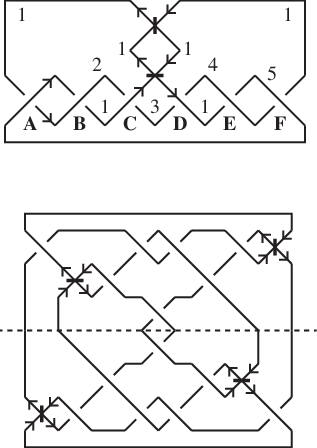
Let $T(2,3)$ denote a torus knot of type $(2,3)$ in ${\mathbb{R}}^{3}$ . Let $T^{0}(2,3)$ denote a 2-sphere in ${\mathbb{R}}^{4}$ that is obtained from $T(2,3)$ by the spinning construction, introduced by Artin [1]. The upper diagram in Figure 8 illustrates a diagram $D^{0}(2,3)$ of an oriented marked graph representing $T^{0}(2,3)$ , denoted by $8_{1}$ in Yoshikawa’s table [16].

Theorem 12.1.

The 0-dimensional Yoshikawa homology of $T^{0}(2,3)$ , $HY_{0}(T^{0}(2,3))$ , is isomorphic to ${\mathbb{Z}}[\mu,\mu^{-1}]\langle x,y\rangle/(\mu(1+\mu)+x-yx,(1+\mu)+\mu y-yx,\mu(1+\mu)+\mu^{-1}x-\mu^{-1}xyx)$ .

Proof.

Arcs of $D^{0}(2,3)$ are labeled by $1,2,3,4,5$ , and crossings of $D^{0}(2,3)$ are labeled by ${\bf A},{\bf B},{\bf C},{\bf D},{\bf E},{\bf F}$ , as illustrated in Figure 8. The diagram $D^{0}(2,3)$ shows that the differential of $(CY_{1}(D^{0}(2,3)),\partial)$ on generators is described as follows.

$\partial c({\bf A},i)=\mu a(1,i)+a(2,i)-a(1,5)a(5,i)$ , $\partial d(i,{\bf A})=a(i,1)+\mu a(1,2)-a(i,5)a(5,1)$ ,

$\partial c({\bf B},i)=\mu a(5,i)+a(1,i)-a(5,2)a(2,i)$ , $\partial d(i,{\bf B})=a(i,5)+\mu a(i,1)-a(i,2)a(2,5)$ ,

$\partial c({\bf C},i)=\mu a(2,i)+a(3,i)-a(2,1)a(1,i)$ , $\partial d(i,{\bf C})=a(i,2)+\mu a(1,3)-a(i,1)a(1,2)$ ,

$\partial c({\bf D},i)=\mu a(4,i)+a(3,i)-a(4,1)a(1,i)$ , $\partial d(i,{\bf D})=a(i,4)+\mu a(i,3)-a(i,1)a(1,4)$ ,

$\partial c({\bf E},i)=\mu a(5,i)+a(1,i)-a(5,4)a(4,i)$ , $\partial d(i,{\bf E})=a(i,5)+\mu a(i,1)-a(i,4)a(4,5)$ ,

$\partial c({\bf F},i)=\mu a(1,i)+a(4,i)-a(1,5)a(5,i)$ , $\partial d(i,{\bf F})=a(i,1)+\mu a(i,4)-a(i,5)a(5,1)$ ,

where $i\in\{1,2,3,4,5\}$ . A direct calculation proves the theorem. ∎

Let $T^{n}(2,3)$ denote a 2-sphere in ${\mathbb{R}}^{4}$ that is obtained from $T(2,3)$ by the twist-spinning construction, introduced by Zeeman [17], where $n\in{\mathbb{Z}}$ . Inoue [6] exhibits an explicit construction of a diagram $D^{n}(2,3)$ of an oriented marked graph representing $T^{n}(2,3)$ . The lower diagram in Figure 8 illustrates a diagram $D^{2}(2,3)$ of an oriented marked graph representing $T^{2}(2,3)$ . A direct calculation shows the following theorem.

Theorem 12.2.

The 0-dimensional Yoshikawa homology of $T^{2}(2,3)$ , $HY_{0}(T^{2}(2,3))$ , is isomorphic to ${\mathbb{Z}}[\mu,\mu^{-1}]\langle x,y\rangle/(\mu(1+\mu)+x-yx,(1+\mu)+\mu y-yx,\mu(1+\mu)+\mu^{-1}x-\mu^{-1}xyx,-(1+\mu)+xy-\mu x,\mu(1+\mu)+y-xy,y+\mu(1+\mu)-y(-\mu(1+\mu)+xy),\mu(1+\mu)+y-\mu^{-1}(-(1+\mu)+xy)(-\mu(1+\mu)+xy),(1+\mu)+\mu x-\mu^{-1}(-(1+\mu)+xy)(-\mu(1+\mu)+xy))$ .

Proof of Theorem 1.2. Theorem 12.1 shows that the algebra map $HY_{0}(T^{0}(2,3))\otimes{\mathbb{Z}}/3{\mathbb{Z}}\to{\mathbb{Z}}/3{\mathbb{Z}}$ is realized by three triples $(\mu,x,y)=(1,2,2),(2,0,0),(2,2,1)$ . Theorem 12.2 shows that $HY_{0}(T^{2}(2,3))\otimes{\mathbb{Z}}/3{\mathbb{Z}}\to{\mathbb{Z}}/3{\mathbb{Z}}$ is realized by two triples $(\mu,x,y)=(1,2,2),(2,0,0)$ . Since the numbers of algebra maps are distinct, $HY_{0}(T^{0}(2,3))$ is not isomorphic to $HY_{0}(T^{2}(2,3))$ . ∎

2-knot homology and Yoshikawa moveThanks: The author is partially supported by JSPS KAKENHI Grant number 15K04865.

Abstract.

1. Introduction

Theorem 1.1.

Theorem 1.2.

2. Definition

Theorem 2.1.

Theorem 2.2.

3. Yoshikawa move Ω1\Omega_{1}

Proposition 3.1.

Proof.

Proposition 3.2.

Proof.

4. Yoshikawa move Ω2\Omega_{2}

Proposition 4.1.

Proof.

5. Yoshikawa move Ω3\Omega_{3}

Proposition 5.1.

Proof.

5.1. Destabilization on (CY(D0),∂)(CY(D_{0}),\partial)

5.2. Destabilization on (CY(D1),∂)(CY(D_{1}),\partial)

5.3. Tame isomorphism between (CY0(D0),∂0)(CY^{0}(D_{0}),\partial^{0}) and (CY1(D1),∂1)(CY^{1}(D_{1}),\partial^{1})

6. Yoshikawa move Ω4\Omega_{4}

Proposition 6.1.

Proof.

7. Yoshikawa move Ω4′\Omega_{4}^{\prime}

Proposition 7.1.

Proof.

8. Yoshikawa move Ω5\Omega_{5}

Proposition 8.1.

Proof.

9. Yoshikawa moves Ω6\Omega_{6}, Ω6′\Omega_{6}^{\prime} and Ω7\Omega_{7}

Proposition 9.1.

Proposition 9.2.

10. Yoshikawa move Ω8\Omega_{8}

Proposition 10.1.

Proof.

11. Proof of Theorem 1.1

12. Examples

Theorem 12.1.

Proof.

Theorem 12.2.

References

3. Yoshikawa move $\Omega_{1}$

4. Yoshikawa move $\Omega_{2}$

5. Yoshikawa move $\Omega_{3}$

5.1. Destabilization on $(CY(D_{0}),\partial)$

5.2. Destabilization on $(CY(D_{1}),\partial)$

5.3. Tame isomorphism between $(CY^{0}(D_{0}),\partial^{0})$ and $(CY^{1}(D_{1}),\partial^{1})$

6. Yoshikawa move $\Omega_{4}$

7. Yoshikawa move $\Omega_{4}^{\prime}$

8. Yoshikawa move $\Omega_{5}$

9. Yoshikawa moves $\Omega_{6}$ , $\Omega_{6}^{\prime}$ and $\Omega_{7}$

10. Yoshikawa move $\Omega_{8}$

References

• [1] E. Artin, Zur Isotope zweidimensionalen Flächen im ℝ4{\mathbb{R}}^{4}, Abh. Math. Sem. Univ. Hamburg 4 (1926) 174–177
• [2] K. Cieliebak, T. Ekholm, J. Latschev, L. Ng, Knot contact homology, String topology, and the Cord algebra, J. Éc. polytech. Math. 145 (2017) 661–780
• [3] T. Ekholm, J. Etnyre, L. Ng, M. Sullivan, Knot contact homology, Geom. Topol. 17 (2013) 975–1112
• [4] T. Ekholm, L. Ng, V. Shende, A complete knot invariant from contact homology, Invent. Math. 211 (2018) 1149–1200
• [5] C. McA. Gordon, T. Lidman, Knot contact homology detects cabled, composite, and torus knots, Proc. Amer. Math. Soc. 145 (2017) 5405–5412
• [6] A. Inoue, A symmetric motion picture of the twist-spun trefoil, Exp. Math. 22 (2013) 15–25
• [7] A. Kawauchi, T. Shibuya, S. Suzuki, Description on surfaces in four-space, I; Normal forms, Math. Sem. Notes Kobe Univ. 10 (1982) 75–125
• [8] C. Kearton, V. Kurlin, All 2-dimensional links in 4-space live inside a universal 3-dimensional polyhedron, Alg. Geom. Topol. 8 (2008) 1223–1247
• [9] J. Kim, Y. Joung, S. Y. Lee, On generating sets of Yoshikawa moves for marked graph diagrams of surface-links, J. Knot Theory Ramif. 24 (2015) 1550018
• [10] S. J. Lomonaco, Jr., The homotopy groups of knots I. How to compute the algebraic 2-type, Pacific J. Math. 95 (1981) 349–390
• [11] L. Ng, Knot and braid invariants from contact homology. I, Geom. Topol. 9 (2005) 247–297
• [12] L. Ng, Knot and braid invariants from contact homology. II, Geom. Topol. 9 (2005) 1603–1637
• [13] L. Ng, Framed knot contact homology, Duke Math. J. 141(2) (2008) 365–406
• [14] L. Ng, A topological introduction to knot contact homology, Contact and symplectic topology, Bolyai Soc. Math. Stud., 26, János Bolyai Math. Soc., Budapest, 2014, 485–530
• [15] F. J. Swenton, On a calculus for 2-knots and surfaces in 4-space, J. Knot Theory Ramif. 10 (2001) 1133–1141
• [16] K. Yoshikawa, An enumeration of surfaces in four-space, Osaka J. Math. 31 (1994) 497–522
• [17] E. C. Zeeman, Twisting spun knots, Trans. Amer. Math. Soc. 115 (1965) 471–495