Asymptotics of $d$-Dimensional Visibility

Consider a configuration of (opaque) objects in space. Two objects are said to be visible from each other if there exists an unobstructed line segment between a point on the first object and a point on the second. We are curious about the maximum number of objects which may be visible from a particular point in space in a worst case scenario. We consider the simple case in which our objects are unit cubes with vertices at integer coordinates, bounded between $0$ and $n$. It is clear that there is a configuration in which you can see at least a quadratic (in $n$) number of cubes: you can see all of the cubes that share a face with the boundary of the $n\times n\times n$ cube simultaneously if there are no other obstructing cubes inside of the grid. There are also clearly a maximum of $n^{3}$ cubes that lie in your range of visibility. However, it is not clear if it is possible to see a number of obstructing cubes that is cubic in $n$.

Although questions of a similar flavor have been asked before, the techniques used to solve them are inapplicable to our context. One famous family of questions (see [1]), namely the Orchard Visibility Problem and its variants, considers a circular orchard bounded by a radius $R$ in which a tree of radius $r<1$ is centered at every lattice point. Both the observer and the center of the orchard are located at the origin. The problem asks what the maximum size of $r$ is for which there exists a line of sight connecting the observer to a point on the boundary of the orchard. In [6], Kruskal demonstrates that there exists such a line of sight if and only if $r<\frac{1}{R^{2}+1}$.

A more general view obstruction problem studied in [5], in which centered at each point in the set $(-\tfrac{1}{2},-\tfrac{1}{2}\dots,-\tfrac{1}{2})+\mathbb{N}^{d}$ in $\mathbb{R}^{n}$ is a centrally symmetric convex body. The bodies are expanded uniformly until they block all rays emanating from the origin and into the open positive cone. The problem has been solved for balls in dimensions $d=2,3,4$.

A related problem considers the observer to be positioned at the origin, and trees to be located at lattice points (with radius $0$). The maximum number of trees visible is in bijection with the number of pairs $(x,y)\in\mathbb{N}^{2}$ such that $\gcd(x,y)=1$, which for an infinitely large orchard is $\frac{6}{\pi^{2}}$ of the trees in the orchard. For $d>2$ dimensions, this generalizes to $\frac{1}{\zeta(d)}$ of the trees, where $\zeta$ is the Riemann zeta function.

The two dimensional version of our problem has been solved in [2], where Brady considers an $n\times n$ axis-aligned grid. Figure 1 shows visibility from the darkened blue square in the lower left hand corner, with the obstructing squares visible from the blue square colored red, and the ones not visible colored yellow. The locus of points visible to the blue square are shaded in green.

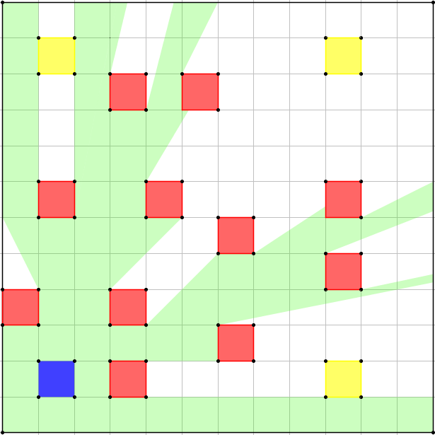
Brady asks: If the number and placement of the obstructing squares in the grid is optimal, then what is the largest number of obstructing squares, as a function of $n$, that can be visible to a given square? Brady used elementary techniques to demonstrate that the answer to this problem is $\Theta(n\sqrt{n})$. To do so, he split the $n\times n$ grid into (mostly) disjoint parallelograms, and computed lower and upper bounds on this maximal value. While the elementary approach used there doesn’t generalize to higher dimensions, we do use the same parallelogram approach in our argument.

In our paper, we generalize the two dimensional bounds Brady obtained to $d>2$ dimensions. In doing so, the two dimensional $n\times n$ grid of squares becomes a $d$-hypercube of side length $n$ consisting of $n^{d}$ unit hypercubes, each of which is either empty or obstructing. Within this larger $d$-hypercube of side length $n$, we seek the maximum possible number of obstructing unit $d$-hypercubes visible from a given obstructing unit $d$-hypercube. It is easiest to visualize this question when $d=3$, and so we shall go about analyzing the problem in three dimensions before extending our results to higher numbers of dimensions. Figure 2 illustrates visibility from the dark blue cube in the case of $d=3$.

Adopting a similar argument to that taken in the two-dimensional case (see [2]), we assume the observer is the cube adjacent to the origin and divide $[0,n]^{3}$ into $1\times 1\times n$ parallelepipeds through the origin to construct a lower bound. By projecting the possible obstructing cubes intersecting the parallelepipeds’ long edges onto the bottom faces of the parallelepipeds, we construct a partially ordered set that characterizes the conditions under which obstructions can block each other. The task of constructing sets of simultaneously visible cubes from the origin is then transformed into one of constructing an antichain of maximal size of a certain partially ordered set. We demonstrate the existence of “small” vectors modulo $n$ that span a lattice corresponding to an antichain of the partially ordered set.

The partially ordered set described above is then modified to model visibility in $d>3$ dimensions. We extend the techniques used in three dimensions to construct a large antichain (coming from a $d-1$ dimensional lattice) of the generalized partially ordered set.

The linear (modulo $p$) structure of the posets considered in Theorem 4.1 is crucial for dimension $d>2$. For any $d$-dimensional poset, one can define a similar family of $2^{d-1}$ related posets by reversing the order on some of the coordinates, and one might be tempted to believe that an analogue of Theorem 4.1 holds for any such situation. When $d=2$, this is indeed true, and it follows easily from the well known Erdős–Szekeres theorem. However, in dimension $d>2$ this is no longer the case. In [9], Szabó and Tardos consider multidimensional generalizations of the Erdős–Szekeres theorem and demonstrate the existence of situations in which all $2^{d-1}$ partially ordered sets in the family of posets have width $O(n^{e_{d}})$ with $e_{d}<1-\tfrac{1}{d}$ for $d\geq 3$ (for instance, their $e_{3}$ is $\tfrac{5}{8}$, which is less than $\tfrac{2}{3}$).

The existence of the partially ordered set from Theorem 4.1 leads to a construction of a configuration in which many obstructions are visible.

As an aside, we note that the $\Omega(n^{1-\tfrac{1}{d}})$ lower bound achieved above matches with the width of a random $d$-dimensional partial order of size $n$, as computed by Brightwell [3] (see discussion of Theorem 2.2 for more).

In approaching an upper bound on the number of visible obstructions, we first consider a reduced visibility environment, in which we restrict visibility to only lines of sight parallel to the edges of the $d$-parallelepiped in consideration. Using the same partially ordered set as used in the lower bound in three dimensions, we demonstrate that there exists a chain cover of sufficiently small size. We do so by studying the value $h_{p}$ defined as follows.

In order to prove these results, we introduce a dual height $h_{p}^{*}$ which is small when there is a simple reason for $h_{p}$ to be large.

Note that if the $t_{i}$ satisfy a simple linear relation such as $at_{1}+bt_{2}+ct_{3}=0{\@displayfalse\pmod{p}}$ with $a,b,c$ small positive constants, then $h_{p}(t)$ must be at least $\frac{p}{(a+b+c)}\sim\frac{p}{max(a,b,c)}$ (up to a factor of $d$). We prove a weak converse to this.

Up to this point, lines of sight under consideration were restricted to just those parallel to the lateral edges of the current parallelotope. We next examine visibility in an environment where this restriction is no longer in place. As we were not able to solve for an upper bound in an unrestricted visibility environment, we weaken the problem.

In Section 2, a brief introduction is given to partially ordered sets. In Section 3, a lower bound on the number of obstructing cubes visible in three dimensions is proven. In Section 4, the bound presented in Section 3 is generalized to $d>3$ dimensions. Section 5 provides an introduction to the so called toy upper bound, a simplification of the true upper bound. In Section 6, a brief introduction is given to the discrete Fourier transform. In Section 7, the results of Sections 5 and 6 are combined to present a bound on visibility in the restricted setting of the toy upper bound in $d>2$ dimensions. Finally in Section 8, an upper bound is presented in a shallow light visibility environment which is stronger than the setting of Section 7 but weaker than the full visibility setting we are interested in.

We first consider the set of parallelepipeds with opposite and parallel square faces, one of which is a unit square whose vertices have integer coordinates on the upper face of the cube, and the other the unit square on the bottom face of the cube with one vertex at the origin. There are $p^{2}$ such parallelepipeds, one for each unit square on the cube’s upper face. Specifically, we are considering parallelepipeds with vertices at coordinates $(0,0,0)$, $(0,1,0)$, $(1,0,0)$, $(1,1,0)$, $(i,j,p)$, $(i+1,j,p)$, $(i,j+1,p)$ and $(i+1,j+1,p)$ where $p$ is the size of the grid, $p$ is a prime number, and $0\leq i,j\leq p-1$.

We now shift our focus to one of these parallelepipeds, call it $\mathcal{P}_{i,j}$, which we shall refer to as simply $\mathcal{P}$ when there is no danger of confusion, whose top face has vertex $(i,j,p)$ closest to the origin. We will refer to $(i,j,p)$ as the characteristic vertex of $\mathcal{P}$. Let $E_{\mathcal{P}_{i,j}}$, or more simply $E_{\mathcal{P}}$ be the edge of $\mathcal{P}_{i,j}$ containing both $(i,j,p)$ and the origin. Denote $E_{\mathcal{P}}$, as well as the other three edges of $\mathcal{P}$ parallel to $E_{\mathcal{P}}$ as the lateral edges of $\mathcal{P}$.

Within $\mathcal{P}$, we will only consider the set of possible obstructing cubes intersecting $E_{\mathcal{P}}$. We additionally restrict visibility to lines of sight parallel to the lateral edges of $\mathcal{P}$. As a result, a line of sight passing through the observer cube is equivalent to the line of sight passing through the bottom face of the observer cube, so we may flatten the observer cube to merely its bottom face without sacrificing any visibility.

The crucial observation is that from the perspective of the observer face, all possible obstructing cubes intersecting the line $E_{\mathcal{P}}$ can be seen only by their bottom face (note that we are not considering all cubes intersecting $\mathcal{P}$, just those which intersect $E_{\mathcal{P}}$ - for the cubes intersecting $\mathcal{P}$ but not $E_{\mathcal{P}}$, this crucial observation is not true). It follows that a set of obstructing cubes, all of which intersect $E_{\mathcal{P}}$, are simultaneously visible to the observer’s face if and only if the same statement is true of their bottom faces.

Note that obstructing cubes near the origin have the potential to be counted as intersecting the lateral edge containing the characteristic vertex for more than some fixed constant number of times as we enumerate over all such $\mathcal{P}$. For this reason, we will further restrict candidates for obstructing cubes to those intersecting the edge $E_{\mathcal{P}}$ of $\mathcal{P}$ that are in the upper half of the parallelepiped, ensuring that each obstructing cube is counted in only a fixed constant number of parallelepipeds. In the following argument however, we will assume that any obstructing cube along $E_{\mathcal{P}}$ is a candidate for being obstructing. This simplification is justified by Proposition 3.1, stating that the width of the partially ordered set modelling visibility for all cubes along $E_{\mathcal{P}}$ is at most a constant factor larger than the partially ordered set modelling visibility along just the upper half of $E_{\mathcal{P}}$.

In this subsection we construct a partially ordered set for $\mathcal{P}_{i,j}$ that models visibility along the edge $E_{\mathcal{P}}$, and whose width is precisely the largest possible number of simultaneously visible obstructions along $E_{\mathcal{P}}$. By switching our choice of $i$ and $j$, the construction can be extended to any such parallelepiped of the form described in Subsection 3.1. In particular, we will show that among the four partially ordered sets attached $\mathcal{P}$ and the parallelepipeds with characteristic vertices $(p-i,j,p)$, $(i,p-j,p)$ and $(p-i,p-j,p)$ respectively, at least one has sufficiently large width.

Consider two square faces at heights $k_{1}$ and $k_{2}$ intersecting $E_{\mathcal{P}}$ and the origin, respectively. When these two squares are projected onto the observer face, the corners are taken to the points $(1-\{\tfrac{ik_{1}}{p}\},1-\{\tfrac{jk_{1}}{p}\},0)$ and $(1-\{\tfrac{ik_{2}}{p}\},1-\{\tfrac{jk_{2}}{p}\},0)$, respectively. It follows that the face at height $k_{1}$ is visible from the observer face if either one of the following conditions are true.

1. 1.

   $k_{1}<k_{2}$ (face $k_{1}$ is lower than face $k_{2}$),

2. 2.

   $1-\{\tfrac{ik_{1}}{p}\}>1-\{\tfrac{ik_{2}}{p}\}$ (the corner face $k_{1}$ “sticks out” from behind face $k_{2}$ with respect to $x$ coordinate),

3. 3.

   $1-\{\tfrac{jk_{1}}{p}\}>1-\{\tfrac{jk_{2}}{p}\}$ (the corner face $k_{1}$ “sticks out” from behind face $k_{2}$ with respect to $y$ coordinate).

Thus, the face at height $k_{2}$ can only block the observer face’s view of the face at height $k_{1}$ if every coordinate of $(1-\{\tfrac{ik_{2}}{p}\},1-\{\tfrac{jk_{2}}{p}\},p-k_{2})$ is larger than the corresponding coordinate in $(1-\{\tfrac{ik_{1}}{p}\},1-\{\tfrac{jk_{1}}{p}\},p-k_{1})$. As a result, a set of obstructing faces all intersecting $E_{\mathcal{P}}$, all of whose elements are simultaneously visible from the observer face, corresponds to an antichain of the partially ordered set $\big\{(\{\tfrac{ik}{p}\},\{\tfrac{jk}{p}\},k)\mid 0\leq k<p\big\}$, under product order. This poset is isomorphic to the much simpler $(ik\pmod{p},jk\pmod{p},k)\mid 0\leq k<p)$ which we shall refer to as $S_{i,j}$. The width of this poset is the maximum number of obstructing cubes intersecting $E_{\mathcal{P}}$ that are all simultaneously visible from the observing face with respect to the restricted lines of sight.

Now consider $\mathcal{P}_{p-i,j}$, $\mathcal{P}_{i,p-j}$ and $\mathcal{P}_{p-i,p-j}$. These parallelepipeds have posets analogous to $S_{i,j}$, with elements of the form $(-ik\pmod{p},jk\pmod{p},k)$, $(ik\pmod{p},-jk\pmod{p},k)$, and $(-ik\pmod{p},-jk\pmod{p},k)$, and which we will denote as $S_{p-i,j}$, $S_{i,p-j}$ and $S_{p-i,p-j}$ respectively. It is then only natural to consider these three partially ordered sets together with $S_{i,j}$ and alternatively their four corresponding parallelepipeds as belonging to the same family. In this manner, the entire set of such parallelepipeds, the size of which is quadratic in $p$, may be partitioned into families of four parallelepipeds.

The proof of Proposition 3.1 can easily be extended to hold true for any partially ordered set of the form $\{(\pm t_{1}k\pmod{p},\dots,\pm t_{m}k\pmod{p},k)\mid 0\leq k<p\}$ for some fixed choice of signs and taken under product order, where $m$ any positive integer.

Our objective now is to find a lower bound on the maximum width among the four posets within the family of $\mathcal{P}$. To bound the width, we show that there exists an antichain of one of the four previously mentioned partially ordered sets of sufficiently large size, and do so in a manner motivated by the following observation. Each element of $S_{i,j}$ may be viewed as a point within $[0,p)^{3}$. Note that just as these points in space are elements of our partially ordered sets, so too are the vectors obtained by taking the difference between any two of these points. From this perspective, we may consider a (shifted) two dimensional lattice of points from the poset as being generated by one element of our poset viewed as a starting point, and two more viewed as vectors. It follows that the intersection of $[0,p)^{3}$ and any such lattice of points from $S_{i,j}$ whose normal vector is of uniform sign corresponds to a maximal antichain of $S_{i,j}$, as the difference between any two elements of this plane is a vector of mixed sign.

As we are working not just with $S_{i,j}$ but with $S_{p-i,j}$, $S_{i,p-j}$, and $S_{p-i,p-j}$ as well it suffices to merely find a lattice (of rank two) within one of the four posets of sufficiently large size. As any lattice within one of the four partially ordered sets exists within the other three albeit with different signs, it remains after such a lattice is found to simply choose the poset whose signs will guarantee the plane to have a normal vector all of whose coordinates are of the same sign.

In the spirit of this, we construct two linearly independent vectors in $S_{i,j}$ with all coordinates as small as possible absolute value wise, and use the lattice spanned by the two vectors to make a statement about the width of one of the four partially ordered sets.

We now construct a second vector in $S_{i,j}$ that is linearly independent from the one found in Lemma 3.1 and that is of sufficiently small size.

In this section, we generalize the results from Section 3 to $d>3$ dimensions. While in three dimensions, we asked how many obstructing cubes could possibly be seen from an observer cube, we now ask how many $d$-hypercubes, which we will abbreviate to just hypercubes when there is no danger of ambiguity, can be seen from an observer $d$-hypercube. The geometric approach is essentially the same.

As in Section 3, we assume that $n=p$ is a prime. We then consider the $d$-hypercube $C$ with side length $p$ formed by $[0,p)^{d}$ and assume that the observer is the unit $d$-hypercube adjacent to the origin.

Consider the vertex $(t_{1},t_{2},\dots,t_{d-1},p)$ on the upper $d-1$-dimensional facet of $C$. This is the $d$-dimensional analogue of the point $(i,j,p)$ (see Section 3). We may then construct the unique $d$-parallelotope $\mathcal{P}$ whose lower base is the bottom $d-1$-dimensional facet of the observer, and which contains the edge with endpoints at the origin and $(t_{1},t_{2},\dots,t_{d-1},p)$. As in Section 3, we refer to the point $(t_{1},t_{2},\dots,t_{d-1},p)$ as the characteristic vertex of $\mathcal{P}$. Additionally we will refer to the segment connecting the characteristic vertex of $\mathcal{P}$ to the origin as $E_{\mathcal{P}}$. For each such choice of $\mathcal{P}$, we will try and maximize the number of obstructing hypercubes intersecting $E_{\mathcal{P}}$ that are simultaneously visible from the observer.

The edge $E_{\mathcal{P}}$ has the special property that any hypercube obstructing $E_{\mathcal{P}}$ is visible to the observer only by its bottom facet, and as a result, any set of obstructing hypercubes intersecting $E_{\mathcal{P}}$ is visible if and only if the corresponding set of bottom facets are also all simultaneously visible. In a near identical manner to Subsection 3.2, it can be seen that the largest number of simultaneously visible obstructing hypercubes along $E_{\mathcal{P}}$ is the width of the set

taken under product order. By considering the family of $d$-parallelotopes whose characteristic vertices can be obtained by switching some of the $t_{i}$’s in $(t_{1},t_{2},\dots,t_{d-1},p)$ to $p-t_{i}$’s, we see that, at a loss of constant factor exponential in $d$, we may for $\mathcal{P}$ consider not just the width of ( † ‣ 4.1), but the maximum of the widths of all posets of the form

taken under product order. Just as in Section 3, we will refer to this collection of posets as the family $S_{\mathcal{P}}$ (see Definition 4.3).

As we enumerate over all such parallelotopes $\mathcal{P}$, we run the risk of counting a given obstructing hypercube in arbitrarily many such parallelotopes. To avoid this, we employ the same technique used in Section 3. Specifically, we restrict the possible obstructing cubes in each parallelotope to the obstructing hypercubes in the upper half of the parallelotope. In other words, we would only consider elements of ( ‡ ‣ 4.1) corresponding to $\frac{p}{2}<k<p$. By Proposition 3.2 , the width of this restricted poset differs from that of ( ‡ ‣ 4.1) by at most a factor of two, so we may ignore this range restriction on $k$ and consider the entirety of the set.

Recall that the argument used in three dimensions (see Section 3) visualized the elements of the given partially ordered set as points within a cube of side length $p$, from which an antichain could be viewed as the intersection between $[0,p)^{3}$ and a lattice whose normal vector had coordinates of uniform sign. In generalizing the results from three dimensions into $d>3$ dimensions, we similarly view the elements of our partially ordered sets as points within a lattice. However the similarities end there, for the argument in Section 3 does not extend directly to higher dimensions, and so a new approach must be taken.

We first recall several important properties of lattices.

For any basis $B=(b_{1},b_{2},\dots,b_{d})$ of a lattice $\mathcal{L}$, let $B^{*}=(b_{1}^{*},b_{2}^{*},\dots,b_{d}^{*})$ be the result when the Gram-Schmidt orthogonalization procedure is applied to $B$ (without normalizing the vectors $b_{i}^{*}$, so the product of their lengths is the covolume of the lattice), and let $\mu_{i,j}=\frac{b_{i}\cdot b_{j}^{*}}{b_{j}^{*}\cdot b_{j}^{*}}$ be the orthogonal projection coefficient of $b_{i}$ onto $b_{j}^{*}$. We now define an LLL reduced basis [7].

One can think of such a basis as being a good approximation of a short orthogonal basis. In [7] it is proved that every lattice has an LLL reduced basis (in fact, an efficient algorithm for finding such a basis is given). If a basis is LLL reduced, Proposition 4.2 can be strengthened to the following proposition, taken from [7] [Proposition $1.6$].

Let $p$ be a prime and let $\mathcal{P}$ be the paralleletope with characteristic vertex $(t_{1},\cdots,t_{d-1},p)$.

Furthermore, observe that the intersection of $\mathcal{L}_{\mathcal{P}}$ with $[0,p)^{d}$ is precisely the multiples of the characteristic vertex $(t_{1},t_{2},\dots,t_{d-1},1)$ taken modulo $p$ and as points in $\mathbb{R}^{d}$.

References

- [1] Thomas Allen “Polya’s orchard problem” In The American Mathematical Monthly 93.2 Taylor & Francis, 1986, pp. 98–104
- [2] Zarathustra Brady “Visible obstructions, parallelograms, and increasing subsequences”, 2010
- [3] Graham Brightwell “Random k-dimensional orders: Width and number of linear extensions” In Order 9.4, 1992, pp. 333–342 DOI: 10.1007
- [4] R.. Dilworth “A Decomposition Theorem for Partially Ordered Sets” In Annals of Mathematics 51.1 Annals of Mathematics, 1950, pp. 161–166 URL: http://www.jstor.org/stable/1969503
- [5] VC Dumir, RJ Hans-Gill and JB Wilker “Contributions to a general theory of view-obstruction problems” In Canadian Journal of Mathematics 45.3 Cambridge University Press, 1993, pp. 517–536
- [6] Clyde Kruskal “The orchard visibility problem and some variants” In Journal of Computer and System Sciences 74.4, 2005 DOI: 10.1016
- [7] A.. Lenstra, H.. Lenstra and L. Lovász “Factoring polynomials with rational coefficients” In Mathematische Annalen 261.4, 1982, pp. 515–534 DOI: 10.1007/BF01457454
- [8] Steven Miller “Heights in Diophantine Geometry by Enrico Bombieri; Walter Gubler” In SIAM Review 49, 2007, pp. 146–148 DOI: 10.2307/20453927
- [9] Tibor Szabó and Gábor Tardos “A Multidimensional Generalization of the Erdős–Szekeres Lemma on Monotone Subsequences” In Combinatorics, Probability and Computing 10.6 Cambridge University Press, 2001, pp. 557–565 DOI: 10.1017/S0963548301004862