Adversarial $\alpha$-divergence Minimization for Bayesian Approximate InferenceJournal: Neurocomputing

Let $\mathbf{w}$ be the latent variables of the model, e.g., the neural network weights. The task of interest in VI is to approximate the posterior distribution of $\mathbf{w}$ given the observed data. For simplicity we will focus on regression models, but the method is broadly applicable to any model and is not limited to neural networks.

Consider a training set $\mathcal{D}=\{\mathbf{x}_{i},y_{i}\}_{i=1}^{N}$, where $\mathbf{x}_{i}$ is some $d$-dimensional input vector and $y_{i}\in\mathds{R}$ is the associated label. The posterior distribution is given by Bayes’ rule:

where $\mathbf{X}$ is a matrix with the observed vectors of input attributes and $\mathbf{y}=(y_{1},\ldots,y_{N})^{\text{T}}$. Furthermore we have assumed i.i.d. data and hence, the likelihood factorizes as $p(\mathbf{y}|\mathbf{w},\mathbf{X})=\prod_{i=1}^{N}p(y_{i}|\mathbf{w},\mathbf{x}_{i})$. In (1) $p(\mathbf{w})$ is the prior distribution of the latent variables of the model (i.e., the neural network weights) and $p(\mathcal{D})=\int p(\mathbf{y}|\mathbf{w},\mathbf{X})p(\mathbf{w})d\mathbf{w}$ is just a normalization constant. In the case of regression problems $p(y_{i}|\mathbf{w},\mathbf{x}_{i})$ is often a Gaussian distribution, i.e., $\mathcal{N}(y_{i}|f(\mathbf{x}_{i}),\sigma^{2})$, where $f(\mathbf{x}_{i})$ is the output of the neural network and $\sigma^{2}$ is the variance of the output noise. Furthermore, $p(\mathbf{w})$ is often a factorizing Gaussian with zero mean and variance $\sigma_{0}^{2}$ (see e.g., [6, 8, 7]). Given (1) the predictive distribution of the model for the label $y^{\star}$ of a new test point $\mathbf{x}_{\star}$ is:

The model prediction would be the expected value of $y^{\star}$ under (2) and the confidence in the prediction can be estimated, e.g., by the standard deviation. In practice, $p(\mathbf{w}|\mathcal{D})$ is intractable because $p(\mathcal{D})$ has no closed form expression and one has to use an approximation to this distribution in (2).

VI approximates (1) using a parametric distribution $q(\mathbf{w})$ which is often a factorizing Gaussian $\mathcal{N}(\mathbf{w}|\bm{\mu},\bm{\Sigma})$ with $\bm{\Sigma}$ a diagonal matrix. Let $\phi$ be the set of parameters of $q(\mathbf{w})$, i.e., $\phi=\{\bm{\mu},\bm{\Sigma}\}$. These parameters are adjusted to minimize the KL divergence between $q(\mathbf{w})$ and the exact posterior (1). Consider the following decomposition of $\log p(\mathcal{D})$:

where $\text{KL}(q(\mathbf{w})||p(\mathbf{w}|\mathcal{D}))$ is the KL divergence between $q(\mathbf{w})$ and the exact posterior:

The KL divergence is always non-negative and is only zero if the two distributions are the same. Therefore, by minimizing this divergence VI enforces that $q(\mathbf{w})$ looks similar to the exact posterior (1).

Because $\log p(\mathcal{D})$ is a constant term independent of $\phi$, the KL divergence between $q(\mathbf{w})$ and the exact posterior can be simply minimized by maximizing the first term in the r.h.s. of (3) with respect to $\phi$. This term is often referred to as the evidence lower bound:

where $\text{KL}(q(\mathbf{w})||p(\mathbf{w}))$ is the KL divergence between $q(\mathbf{w})$ and the prior $p(\mathbf{w})$. If $q(\mathbf{w})$ and the prior are Gaussian, there is a closed form expression for this divergence. The maximization of (5) can be done using stochastic optimization techniques that sub-sample the training data and that approximate the required expectations using Monte Carlo samples (see [8] for further details). The hyper-parameters of the model, i.e., the noise and prior variance $\sigma^{2}$ and $\sigma_{0}^{2}$ are estimated by maximizing $\mathcal{L}(\phi)$, which approximates $\log p(\mathcal{D})$ since $\text{KL}(q(\mathbf{w})||p(\mathbf{w}|\mathcal{D}))$ is expected to be fairly small. Finally, after training, the posterior approximation can replace the exact posterior in (2) and the predictive distribution for new data can be approximated by a Monte Carlo average over the posterior samples.

AVB extends VI to account for implicit models for the approximate distribution $q(\mathbf{w})$. An implicit model for $q(\mathbf{w})$ is a distribution that is easy to generate samples from, but that lacks a closed form expression for the p.d.f. An example is a source of standard Gaussian noise that is non-linearly transformed by a neural network. That is,

where $\mathbf{f}_{\phi}(\bm{\epsilon})$ is the output of a neural network that receives $\bm{\epsilon}$ at the input and $\delta(\cdot)$ is a delta function. In general, the integral in (6) is intractable due to the strong non-linearities of the neural network. Nevertheless, it is very easy to generate $\mathbf{w}\sim q_{\phi}$. For this, one only has to generate $\bm{\epsilon}\sim\mathcal{N}(\mathbf{0},\mathbf{I})$ to then compute $\mathbf{w}=\mathbf{f}_{\phi}(\bm{\epsilon})$. If the noise dimension is large enough and $\mathbf{f}_{\phi}(\cdot)$ is flexible enough, any probability distribution can be described like this. Therefore, implicit models can alleviate the approximation bias of VI with parametric distributions $q(\mathbf{w})$.

Using an implicit distribution in VI is challenging because the lower bound in (5) cannot be easily evaluated nor optimized. The reason is that the term $\text{KL}(q(\mathbf{w})||p(\mathbf{w}))$, i.e., the KL divergence between the approximate distribution $q(\mathbf{w})$ and the prior requires the p.d.f. of $q(\mathbf{w})$. AVB provides an elegant solution to this problem. The aforementioned term can be written as:

where $T(\mathbf{w})$ is simply the log-ratio between $q_{\phi}$ and the prior. AVB proposes to estimate this log-ratio as the output of another neural network that discriminates between samples of $\mathbf{w}$ generated from $q_{\phi}$ and from the prior [10]. This technique has also been considered in other works [13, 16, 14]. Let $T_{\omega}(\cdot)$ be the output of the discriminator. The following objective is considered for optimizing the discriminator assuming $q_{\phi}(\mathbf{w})$ is fixed:

where $\sigma(\cdot)$ is the sigmoid-function. Roughly speaking, this objective tries to make the discriminator differentiate between samples generated from $q_{\phi}(\mathbf{w})$ and from the prior $p(\mathbf{w})$.

If the discriminator $T_{\omega}$ is considered flexible enough to represent any function of $\mathbf{w}$, it is possible to prove that the optimal discriminator behaves as expected by providing the correct log-ratio between the two distributions. If we rewrite (8) making explicit the dependence on both $q_{\phi}(\mathbf{w})$ and $p(\mathbf{w})$ we obtain

This integral is maximal for $T_{\omega}(\mathbf{w})$ if and only if the integrand is maximal for every $\mathbf{w}$ value. The shape of the integrand is:

for $a=q_{\phi}(\mathbf{w})$, $b=p(\mathbf{w})$, and $t=T_{\omega}(\mathbf{w})$. Its maximum value is attained at $t=\frac{a}{a+b}$. Therefore, the optimal solution $T_{\omega^{\star}}$ is

or equivalently,

which is the result desired to correctly estimate the KL divergence between $q_{\phi}$ and the prior. In particular, the discriminator can be plugged in (7) and the expectation can be approximated simply by a Monte Carlo average by generating samples from $q_{\phi}$.

Given $T_{\omega^{\star}}$ the lower bound employed in AVB is obtained by re-writing the evaluation of the KL divergence between $q_{\phi}$ and the prior:

Note that all the required expectations can be simply approximated by generating samples from $q_{\phi}$ and the sum across the training data can be approximated using mini-batches. This lower bound can be hence easily maximized w.r.t. $\phi$ using stochastic optimization techniques. For this, however, we need to differentiate the stochastic estimate with respect to $\phi$. This may seem complicated since $T_{\omega^{\star}}(\mathbf{w})$ is defined as the solution of an auxiliary optimization problem that depends on $\phi$. However, due to the expression for the optimal discriminator, it can be showed that $\mathds{E}_{q_{\phi}(\mathbf{w})}\left(\nabla_{\phi}T_{\omega^{\star}}(\mathbf{w})\right)=0$. Therefore the dependence of $T_{\omega^{\star}}(\mathbf{w})$ w.r.t $\phi$ can be ignored. See [10] for further details. In practice, both $q_{\phi}$ and the discriminator $T_{\omega}(\mathbf{w})$ are trained simultaneously. However, $q_{\phi}$ is updated by maximizing (13) using a smaller learning rate than the one used to update the discriminator $T_{\omega}$, which considers the objective in (8). This helps achieving that $T_{\omega}$ is an accurate estimator of the log-ratio between $q_{\phi}$ and the prior, and that the KL divergence is correctly estimated when updating $q_{\phi}$.

AVB relies on a good approximation $T_{\omega}(\mathbf{w})$ to the optimal discriminator. Although in the non-parametric limit this is achieved, in practice $T_{\omega}(\mathbf{w})$ can fail to be sufficiently close to the optimal discriminator. This a consequence of AVB calculating the discriminator between $q_{\phi}$, the posterior approximation and the prior, which are often very different distributions. This results in practice in a more relaxed performance of the estimated discriminator, which has no problem telling apart samples from one density or the other, but that fails to correctly estimate the log-ratio between probability distributions.

In [10] a solution is proposed, which consists in introducing a new auxiliary conditional probability distribution $r_{\alpha}(\mathbf{w})$ with known density that approximates $q_{\phi}$. This auxiliary distribution is set to be a factorizing Gaussian whose mean and variances match those of $q_{\phi}$. Using this extra distribution, the objective in (5) is rewritten as

If $r_{\alpha}(\mathbf{w})$ approximates well $q_{\phi}(\mathbf{w})$, the KL divergence between these distributions will often be much smaller than $\text{KL}(q_{\phi}(\mathbf{w})||p(\mathbf{w}))$, which facilitates learning the correct probability ratio.

This technique is called adaptive contrast, because the divergence is not being calculated between $q_{\phi}$ and the prior, but between $q_{\phi}$ and the adaptive distribution $r_{\alpha}$. Therefore, the discriminator now estimates $\text{KL}(q_{\phi}(\mathbf{w})||r_{\alpha}(\mathbf{w}))$ and hence the log-ratio between $q_{\phi}$ and $r_{\alpha}$. More precisely, introducing this new auxiliary distribution, the lower bound becomes

where now $T_{\omega}(\mathbf{w})$ approximates the optimal discriminator between samples from $r_{\alpha}(\mathbf{w})$ and $q_{\phi}(\mathbf{w})$. Moreover, the KL divergence in (14) is invariant under any change of variables. Therefore, it can be rewritten as:

where $\tilde{q}_{\phi}(\tilde{\mathbf{w}})$ is the distribution of the standardized vector $\tilde{\mathbf{w}}$, whose $j$-th component is given by $\tilde{w}_{j}\coloneqq\frac{w_{j}-\mu_{j}}{\sqrt{\Sigma_{j,j}}}$ (with $\mu_{j}$ and $\Sigma_{j,j}$ the mean and variance of $w_{j}$, respectively), and $r_{0}(\tilde{\mathbf{w}})$ is a standard Gaussian distribution. Therefore, the discriminator $T_{\omega}(\mathbf{w})$ just needs to look for differences between samples from the normalized posterior approximation and from a standard Gaussian distribution. The mean and variances of $\mathbf{w}$ under $q_{\phi}$ can simply be estimated using samples from this distribution.

We consider the objective function of a general method for approximate inference known as power expectation propagation (PEP) [22]. PEP allows for minimizing $\alpha$-divergences in an approximate way, but constrains the approximate distribution $q(\mathbf{w})$ to belong to the family of exponential distributions (e.g., $q(\mathbf{w})$ is a Gaussian distribution). More precisely, the global minimization of the $\alpha$-divergence is intractable, except when $\alpha\rightarrow 0$ (see [18] for further details). Let the unnormalized target distribution be the product of several factors, i.e., $p\propto\prod_{i}f_{i}$. If we have i.i.d. data, this is always the case, since the likelihood factorizes. PEP approximates $p(\mathbf{w}|\mathcal{D})$ by $q(\mathbf{w})$, which is written as a product of simple factors $q\propto\prod_{i}\tilde{f}_{i}$. Each $\tilde{f}_{i}$ belongs to the exponential family (e.g. a Gaussian factor) and approximates the corresponding exact factor $f_{i}$. PEP minimizes the $\alpha$-divergence locally, instead of globally. In particular, PEP minimizes the $\alpha$-divergence between the tilted distributions of the model, and the approximate distribution $q(\mathbf{w})$. The tilted distributions of the model are those distributions in which one approximate factor $\tilde{f}_{i}$ is replaced by the corresponding exact factor $f_{i}$. Namely, $p^{\setminus j}\propto f_{j}\prod_{i\neq j}\tilde{f}_{i}$. Therefore, PEP minimizes $D_{\alpha}[p^{\setminus j}|q]$ for all $j$. In general, it is expected that a local minimization of the $\alpha$-divergence gives similar results to a global minimization while being a much simpler problem, as indicated in [18].

To perform the local minimization of the $\alpha$-divergence PEP optimizes the following objective function:

where $Z_{q}$ is the normalization constant of $q_{\phi}$, $Z_{p(\mathbf{w})}$ is the normalization constant of the prior, $\phi$ are the parameters of $q(\mathbf{w})$ and $\{\theta_{i}\}_{i=1}^{N}$ are the parameters of the approximate factors $\tilde{f}_{i}$. In this case, we have assumed that the prior distribution need not be approximated and already belongs to the exponential family (i.e., it is a Gaussian prior). When $\alpha\rightarrow 0$, (21) converges to the lower bound of VI in (5) [18]. Therefore, a local minimization of the KL divergence employed in VI is equivalent to a global minimization.

In practice, PEP solves the problem $\max_{\phi}\,\,\min_{\{\theta_{i}\}_{i=1}^{N}}\mathcal{L}(\phi,\{\theta_{i}\}_{i=1}^{N})$, which is a complicated task since it requires a slow double loop algorithm [23]. Furthermore, PEP does not scale to big data since it maintains an approximate factor associated to each likelihood factor, which results in a space complexity of $\mathcal{O}(N)$.

Black-box-$\alpha$ (BB-$\alpha$) is an improvement over the previous method, PEP, that addresses some of its limitations like the memory space requirements and also allows to make approximate inference on complicated probabilistic models [7]. For this, the PEP objective function is rewritten as:

where now there is only one approximate factor $\tilde{f}(\mathbf{w})$ that is replicated $N$ times, one per each complicated likelihood factor. Therefore, $q_{\phi}(\mathbf{w})\propto\tilde{f}(\mathbf{w})^{N}p(\mathbf{w})$. This solves the problem of having to store in memory the parameters of $N$ factors. Furthermore, there is a one to one map between $\tilde{f}(\mathbf{w})$ and $q_{\phi}(\mathbf{w})$. This means that the max-min optimization problem of PEP is transformed into just a standard maximization problem (w.r.t to the parameters of $q(\mathbf{w})$, $\phi$), which can be solved using standard optimization techniques. Importantly, the expectations in (22) can be approximated via Monte Carlo sampling and the sum across the training data can be approximated using a mini-batch. The consequence is that BB-$\alpha$ scales to big datasets, as (22) can be optimized using stochastic techniques, and moreover, it can be applied to complicated probabilistic models (e.g., Bayesian neural networks) in which the required expectations are intractable. Again, when $\alpha\rightarrow 0$ (22) converges to the lower bound of VI in (5). When $\alpha=1$, (22) is approximately equal to the objective optimized by Expectation Propagation [7]. A limitation of BB-$\alpha$ is, however, that the approximate distribution $q(\mathbf{w})$ is restricted to be inside the exponential family. This is because it must be written as the product of an approximate factor times the prior distribution. That is, $q_{\phi}(\mathbf{w})\propto\tilde{f}(\mathbf{w})^{N}p(\mathbf{w})$. This is a major limitation that makes difficult using implicit models for $q(\mathbf{w})$.

In this section we will do an analogous reparametrization for the general expression of the BB-$\alpha$ objective suggested in [21] for VI, but we will instead apply it to AVB. This reparametrization will allow to approximately minimize $\alpha$-divergences with flexible distributions $q(\mathbf{w})$ such as the ones resulting from implicit models. Therefore, it will enable us to complete the formulation of our model by making use of this type of divergences, extending on the existing formulation of AVB. To this end, first consider the following alternative expression for the BB-$\alpha$ objective:

In this expression we observe that the hypothesis that $q_{\phi}(\mathbf{w})\propto\tilde{f}^{N}(\mathbf{w})p(\mathbf{w})$ is not required anymore (both $Z_{q}$ and $\tilde{f}(\mathbf{w})$ are removed from the expression) and $q(\mathbf{w})$ can be an arbitrary distribution. It is possible to show that (23) and (22) become equivalent if $q(\mathbf{w})$ belongs to the exponential family [21]. A difficulty is, however, that this expression requires the evaluation of the density $q_{\phi}(\mathbf{w})$ which in practice can be hard to compute.

To overcome the limitation described before, in [21], they reparametrize (23) using the so-called cavity distribution. That is, the distribution given by the ratio $q_{\phi}/\tilde{f}^{\alpha}$. If $\tilde{q}_{\phi}(\mathbf{w})$ denotes a free-form cavity distribution, the posterior approximation $q_{\phi}$ is given by:

where we assume $Z_{q}<+\infty$ is the normalizing constant to make $q(\mathbf{w})$ a valid distribution. When $\alpha/N\rightarrow 0$ we have that $q\rightarrow\tilde{q}$ (and $Z_{q}\rightarrow 1$ by assumption), and this is the case either if we choose $\alpha\rightarrow 0$ or for a sufficiently large $N$ (i.e. $N\rightarrow+\infty$), see [21]. We rewrite now (23) in terms of $\tilde{q}$ rather than $q(\mathbf{w})$:

where $\beta=N/(N-\alpha)$ and $\text{R}_{\beta}[\tilde{q}|p]$ represents the Rényi divergence of order $\beta$ [24], which is defined as

Importantly, when $\alpha/N\rightarrow 0$ we recover $q\rightarrow\tilde{q}$ and $\mathcal{L}_{\alpha}(\phi)$ converges to the objective of VI. Also, we have that $\text{R}_{\beta}[\tilde{q}|p]\rightarrow\text{KL}[\tilde{q}||p]=\text{KL}[q||p]$ if $\text{R}_{\beta}[\tilde{q}|p]<+\infty$ (which is true assuming $Z_{q}<+\infty$ and $\alpha/N\rightarrow 0$). Therefore, when this quotient tends to zero, we can make further approximations for the BB-$\alpha$ energy function as described in (23), finally obtaining

This will be the objective function that we will optimize in our approach. Note that the expectations in (27) can be estimated via Monte Carlo sampling. In particular, $\log\mathds{E}_{q_{\phi}(\mathbf{w})}[p(y_{i}|\mathbf{x}_{i},\mathbf{w})^{\alpha}]\approx\log[K^{-1}\sum_{k=1}^{K}p(y_{i}|\mathbf{x}_{i},\mathbf{w}_{k})^{\alpha}]$, for $K$ samples of $\mathbf{w}$ drawn from $q_{\phi}$. Of course, this estimate is biased, as a consequence of the non-linearity of the $\log(\cdot)$ function, however, the bias can be controlled with $K$. Furthermore, we expect a similar behavior as in standard BB-$\alpha$, in which the bias has been shown to be very small even for $K=10$ samples. See [7] for further details.

The objective in (27) has been obtained under some conditions that need not be true in practice, e.g. the quotient $\alpha/N\rightarrow 0$ (i.e., either $\alpha$ is small, $N$ is sufficiently large or a combination of both). Nevertheless, it is much simpler to estimate and optimize than the one in (23). It is also similar to the objective functions found in the deep learning bibliography (i.e., a loss function plus some regularizer, i.e., the KL divergence), but it still maintains the qualities of an approximate Bayesian inference algorithm. Importantly, (27) allows for implicit models for $q_{\phi}$. The only term that is difficult to approximate is $\text{KL}[q_{\phi}(\mathbf{w})||p(\mathbf{w})]$. However, the approach described in Section 2.2 can be used for that purpose. By changing the $\alpha$ parameter of the method we will be able to interpolate between AVB ($\alpha\rightarrow 0$) and an EP like algorithm ($\alpha=1$). Note that when $\alpha\rightarrow 0$, (27) is expected to focus on reducing the training error since the factor $\alpha^{-1}\log\mathds{E}_{q_{\phi}(\mathbf{w})}[p(y_{i}|\mathbf{x}_{i},\mathbf{w})^{\alpha}]$ will converge to $\mathds{E}_{q_{\phi}(\mathbf{w})}[\log p(y_{i}|\mathbf{x}_{i},\mathbf{w})]$, with $p(y_{i}|\mathbf{x}_{i},\mathbf{w})$ typically a Gaussian distribution with mean given by the output of the neural network and noise variance $\sigma^{2}$. By contrast, when $\alpha=1$, (27) will be expected to focus more on the training log-likelihood. Intermediate values of $\alpha$ will trade-off between these two tasks, which may lead to better generalization properties.

With respect to the specific details of the architecture of the proposed approach, it consists of a structure analogous to the one presented in AVB [10]. Therefore, its structure can be divided into three networks: An implicit model for $q_{\phi}$, which takes as input Gaussian noise and outputs neural network weight samples $\mathbf{w}$ from the approximated weights posterior distribution (i.e., the generator network); a discriminator, which estimates the KL term present in (27) as done in [10]; and finally the main network, that uses the samples of the weights generated previously to evaluate the factor $p(y_{i}|\mathbf{x}_{i},\mathbf{w})$. The whole system is optimized all together. Furthermore, any potential hyper-parameter (e.g., the prior variance $\sigma_{0}^{2}$ or the output noise variance $\sigma^{2}$) is tuned simply by maximizing (27).

Finally, as a last remark concerning the implementation of the proposed method, we have also included as trainable parameters both the mean and variances of the Gaussian noise which is used as input in the generator network (the implicit model for the weights, $q_{\phi}(\mathbf{w})$, in (6)), $\bm{\epsilon}\sim\mathcal{N}(\bm{\mu}_{\text{noise}},\bm{\Sigma}_{\text{noise}})$, with $\bm{\Sigma}_{\text{noise}}$ a diagonal matrix. This allows for a more expressive implicit model for $q_{\phi}(\mathbf{w})$, since it increases its flexibility by allowing the tuning of the broad parameters that control its input. Using this, the model is expected to reproduce to a higher degree of accuracy the original posterior distribution of the model parameters (neural network weights).

In order to analyze the behavior of the proposed method we evaluate the AADM on two simple regression problems extracted from [35]. More precisely, we generate two different toy datasets. The first one involving a heteroscedastic predictive distribution, and the second one involving a bimodal predictive distribution.

The structure of the system employed is the one described previously. We train this system for 3000 epochs, using the first 500 epochs as the warm-up period. We repeat the experiments for different values of alpha in the $(0,1]$. The first dataset is generated taking $x$ uniformly distributed in the interval $[-4,4]$ and $y$ is obtained as $y=7\sin x+3|\cos(x/2)|\epsilon$, where $\epsilon$ is normally-distributed and independent of $x$, i.e., $\epsilon\sim\mathcal{N}(0,1)$. Note that this dataset involves input dependent noise. The second dataset uses $x$ uniformly distributed in the interval$[-2,2]$ and $y=10\sin x+\epsilon$ with probability $0.5$ and $y=10\cos x+\epsilon$ otherwise. The distribution of $\epsilon$ is the same as in the first dataset. note that this other dataset involves a bimodal predictive distribution. We use 1000 data instances for training and the mini-batch size is set to 10.

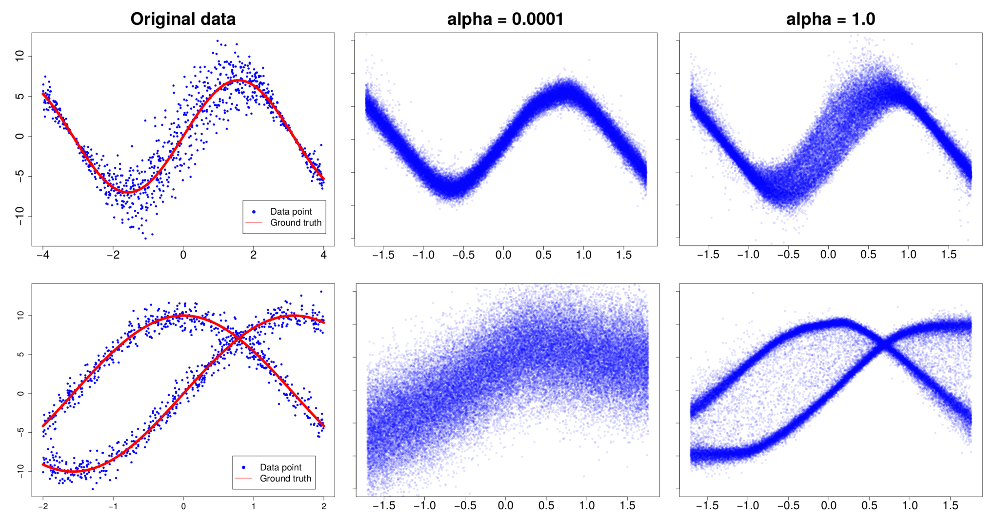
The results obtained in the synthetic problems described are represented in Figure 2. The top figures correspond to the problem involving the heteroscedastic noise and the bottom ones to the problem with a bimodal predictive distribution. On the left of the figure we show the original data we used to train AADM. In these plots, the red lines represent the ground truth for each dataset and the blue points are the actual samples we used as training data. The middle and right columns show samples from the predictive distribution of a neural network trained using AADM, for $\alpha=10^{-4}$ and $\alpha=1$, respectively. The results obtained for $\alpha=10^{-4}$ are expected to be equal to those of AVB. As can be noticed, a low value of alpha is unable to reproduce the complex structure of the data, losing main qualities such as the heteroscedastic additive noise in the first task and the bimodality of the predictive distribution in the second task. However, both of them are recovered with accuracy when alpha is higher, which is showcased by the results obtained when $\alpha=1$.

The results obtained in these experiments, although synthetic, already show that choosing one value of $\alpha$ or another, for the divergence that is approximately optimized in AADM can significantly change the results obtained. In particular, when $\alpha=10^{-4}$ we can observe that the predictive distribution that is obtained (after fitting the posterior approximation) focuses more on minimizing the squared error and less on the log-likelihood of the data. By contrast, when $\alpha=1.0$, the predictive distribution plays a closer attention to the log-likelihood of the data, and can hence obtain a more accurate predictive distribution. As can be seen in Table 1, although the squared error obtained when $\alpha=10^{-4}$ and $\alpha=1.0$ is very similar, the test log-likelihood obtained when $\alpha=1.0$ is much better, which indicates that this value of $\alpha$ produces more accurate predictive distributions. Note that the squared error only measures the expected squared deviation from target value. The test log-likelihood, on the other hand, measures the overall quality of the predictive distribution, taking into account, for example, features such as multiple-modes, heavy-tails or skewness.

Finally, other values of $\alpha$ give similar results (not shown here). In particular, for $\alpha<0.5$ similar results to those of $\alpha=10^{-4}$ are obtained. By contrast, when $\alpha>0.5$ similar results to those of $\alpha=1.0$ are obtained (that is, only if the training procedure is carried out carefully to avoid bad local optima).

To analyze in more detail the results of the proposed method, AADM, we have considered eight UCI datasets [33] that are widely spread for regression [6]. The characteristics of these datasets are displayed in Table 2. Each dataset has a different size, and in order to train the different methods until convergence we have employed a different number of epochs in each case. The number of epochs selected is presented finally in Table 2. Note that, even though there are differences in the epochs employed for training, all of the datasets share the same model structure, which is the general one described at the beginning of this section. In all these experiments we employ the first $10\%$ of the total training epochs for warming-up before the KL term is completely turned on as in [25]. Moreover, the batch size is set to be 10 data points, and sampling-wise, we perform 10 samples in the training procedure and 100 for testing. We split the datasets in a 90%-10% for training/testing. The results reported are averages over 20 different random splits of the datasets into training and testing.

We compare the results of AADM with VI using a factorizing Gaussian as the posterior approximation and with regular AVB (which should be the same as our algorithm when $\alpha\rightarrow 0$). For all methods we employ the same two-layered system with 50 units per layer. To make fair comparisons we also perform the same warm-up period for both AVB and VI as we use in our method. Therefore only after the first 10% of the total number of epochs, the KL term is completely activated in the objective function.

The average performance of each method on each dataset, in terms of the test log-likelihood, is displayed Figure 3. The test log-likelihood measures the overall quality of the predictive distribution, taking into account, for example, features such as multiple-modes, heavy-tails or skewness. We observe that values of $\alpha$ that are different from $0$ usually outperform both regular AVB and VI in terms of this metric (the higher the values the better). From these figures, it seems that higher values of $\alpha$ often lead to better predictive distributions it terms of the test log-likelihood, probably as a consequence of being able to better recover the real posterior distribution. The values obtained are similar and often better than those of other state of the art methods [6]. Each of the values shown represent the mean performance of a certain method across the 20 different splits of each dataset, which are averaged afterwards here. Importantly, we observe that standard VI is almost always outperformed by the two techniques that allow for implicit models in the posterior approximation $q(\mathbf{w})$. Namely, AVB and AADM. This points out the benefits of using an implicit model for the approximate distribution $q(\mathbf{w})$. Moreover, AVG and AADM give almost the same results when $\alpha\approx 0$, which confirms the correctness of our implementation.

The average results obtained for each method on each dataset, in terms of the root mean squared error (RMSE) are displayed in Figure 4. Note that the root mean squared error only measures the expected deviation from the target value and it may ignore if the model captures accurately the distribution of the target value. We can see that the proposed approach, AADM, also obtains better results than VI. In this case, nonetheless, different $\alpha$ values do not actually improve much over the basic results of AVB, and in general we can see that lower values for $\alpha$ are actually better to obtaining a good performance in terms of this metric (here, the lower in the graphs the better the performance). This seems to indicate that one should choose a value for $\alpha$ that is different, depending on the metric they are most interested in. These results are consistent in the sense that, as pointed out previously, values of $\alpha$ close to zero actually lead to the objective that is optimized in AVB and VI, which pays more attention to the training RMSE, in the case of regression problems with Gaussian noise. By contrast, values of $\alpha$ closer to one, pay more attention to the log-likelihood of the training data.

To evaluate the performance of the proposed method on large datasets, we have carried out additional experiments considering two datasets: Airlines Delay, and Year Prediction MSD. Airlines Delay contains information about all commercial flights in the USA from January 2008 to April 2008 [36]. The task of interest is to predict the delay in minutes of a flight based on 8 attributes: age of the aircraft, distance that needs to be covered, air-time, departure time, arrival time, day of the week, day of the month and month. This is hence a very noisy dataset. After removing instances with missing values, $2,127,068$ instances remain. From these, $10,000$ are used for testing and the rest are used for training. Year Prediction MSD is publicly accessible on the UCI repository [33]. This dataset has $515,345$ data instances and $90$ attributes. Again, we use $10,000$ for testing and the rest of the data are used for training. In these experiments the mini-batch size has been set to 100 and we have not used the warm-up annealing scheme that deactivates the KL term in the objective of each method during the initial training iterations. For each method, we measured the performance in the test set, in terms of the RMSE and the test log-likelihood, as a function of the training time.

The results obtained for each method on the Airlines dataset are displayed in Figure 6. In this figure dashed lines represent other methods, the black being AVB and the blue VI. Solid lines represent our method, AADM, for different values of alpha. The figure shows that AADM obtains better results than AVB and VI in terms of the test log-likelihood when $\alpha$ approaches $1$. When $\alpha$ is closer to $0$, AADM, gives similar results to those of AVB and VI in the long term. The performance of our method w.r.t. the computational time is comparable to that of AVB. In terms of RMSE, however, large values of $\alpha$ seem to exhibit a more unstable behavior and in general give worse results. This is probably a consequence of this dataset being very noisy.

The results obtained for each method on the Year dataset are displayed in Figure 7. Again, in this figure dashed lines represent other methods, the black being AVB and the blue VI. Solid lines represent our method, AADM, for different values of alpha. As in the previous dataset, AADM obtains better results than AVB and VI in terms of the test log-likelihood when $\alpha$ approaches $1$. When $\alpha$ is closer to $0$, AADM, gives similar results to those of AVB and VI. In terms of RMSE, lower values of $\alpha$ seems to give also the best results. However, in this case higher values of $\alpha$ do not seem to give significantly worse results in terms of this metric.

References

- [1] Y. LeCun, Y. Bengio, G. Hinton, Deep learning, Nature 521 (2015) 436–444.
- [2] A. Krizhevsky, I. Sutskever, G. E. Hinton, Imagenet classification with deep convolutional neural networks, in: Advances in Neural Information Processing Systems, 2012, pp. 1097–1105.
- [3] S. Hochreiter, J. Schmidhuber, Long short-term memory, Neural computation 9 (1997) 1735–1780.
- [4] Y. Gal, Uncertainty in deep learning, Ph.D. thesis, PhD thesis, University of Cambridge (2016).
- [5] R. M. Neal, Bayesian learning for neural networks, Vol. 118, Springer Science & Business Media, 2012.
- [6] J. M. Hernández-Lobato, R. P. Adams, Probabilistic backpropagation for scalable learning of Bayesian neural networks, in: International Conference on Machine Learning, 2015, pp. 1861–1869.
- [7] J. M. Hernández-Lobato, Y. Li, M. Rowland, D. Hernández-Lobato, T. D. Bui, R. E. Turner, Black-box -divergence minimization (2016) 1511–1520.
- [8] A. Graves, Practical variational inference for neural networks, in: Advances in neural information processing systems, 2011, pp. 2348–2356.
- [9] D. J. Rezende, S. Mohamed, Variational inference with normalizing flows, in: International Conference on Machine Learning, 2016, pp. 1530–1538.
- [10] L. Mescheder, S. Nowozin, A. Geiger, Adversarial variational bayes: Unifying variational autoencoders and generative adversarial networks, in: International Conference on Machine, 2017, pp. 2391–2400.
- [11] Q. Liu, D. Wang, Stein variational gradient descent: A general purpose Bayesian inference algorithm, in: Advances In Neural Information Processing Systems, 2016, pp. 2378–2386.
- [12] T. Salimans, D. Kingma, M. Welling, Markov chain Monte Carlo and variational inference: Bridging the gap, in: International Conference on Machine Learning, 2015, pp. 1218–1226.
- [13] D. Tran, R. Ranganath, D. Blei, Hierarchical implicit models and likelihood-free variational inference, in: Advances in Neural Information Processing Systems, 2017, pp. 5523–5533.
- [14] Y. Li, Q. Liu, Wild variational approximations, in: NIPS workshop on advances in approximate Bayesian inference, 2016.
- [15] M. J. Beal, Variational algorithms for approximate Bayesian inference, Ph.D. thesis (2003).
- [16] F. Huszár, Variational inference using implicit distributionsArXiv preprint arXiv:1702.08235.
- [17] S. Amari, Differential-geometrical methods in statistics, Vol. 28, Springer Science & Business Media, 2012.
- [18] T. Minka, Divergence measures and message passing, Tech. rep., Technical report, Microsoft Research (2005).
- [19] B. J. Frey, R. Patrascu, T. Jaakkola, J. Moran, Sequentially fitting“inclusive”trees for inference in noisy-or networks, in: Advances in Neural Information Processing Systems, 2001, pp. 493–499.
- [20] T. P. Minka, Expectation propagation for approximate bayesian inference, in: Uncertainty in Artificial Intelligence, 2001, pp. 362–369.
- [21] Y. Li, Y. Gal, Dropout inference in bayesian neural networks with alpha-divergences, in: International Conference on Machine Learning, 2017, pp. 2052–2061.
- [22] T. P. Minka, Power EP, Tech. rep., Technical report, Microsoft Research, Cambridge (2004).
- [23] T. Heskes, O. Zoeter, Expectation propagation for approximate inference in dynamic Bayesian networks, in: Uncertainty in Artificial Intelligence, 2002, pp. 216–223.
- [24] A. Rényi, On measures of entropy and information, in: Fourth Berkeley Symposium on Mathematical Statistics and Probability, Vol. 1, 1961, pp. 547–561.
- [25] C. K. Sønderby, T. Raiko, L. Maaløe, S. K. Sønderby, O. Winther, Ladder variational autoencoders, in: Advances in neural information processing systems, 2016, pp. 3738–3746.
- [26] S. Duane, A. D. Kennedy, B. J. Pendleton, D. Roweth, Hybrid Monte Carlo, Physics letters B 195 (1987) 216–222.
- [27] R. M. Neal, MCMC using Hamiltonian dynamics, in: Handbook of Markov chain Monte Carlo, 2011, pp. 113–162.
- [28] M. I. Jordan, Z. Ghahramani, T. S. Jaakkola, L. K. Saul, An introduction to variational methods for graphical models, Machine learning 37 (1999) 183–233.
- [29] D. Soudry, I. Hubara, R. Meir, Expectation backpropagation: Parameter-free training of multilayer neural networks with continuous or discrete weights, in: Advances in Neural Information Processing Systems, 2014, pp. 963–971.
- [30] M. D. Hoffman, Learning deep latent Gaussian models with Markov chain Monte Carlo, in: Proceedings of the 34th International Conference on Machine Learning-Volume 70, 2017, pp. 1510–1519.
- [31] M. K. Titsias, F. J. R. Ruiz, Unbiased implicit variational inference, in: Artificial Intelligence and Statistics, 2019, pp. 167–176.
- [32] Y. Gal, Z. Ghahramani, Dropout as a Bayesian approximation: Representing model uncertainty in deep learning, in: International Conference on Machine Learning, 2016, pp. 1050–1059.
- [33]
D. Dua, C. Graff, UCI machine learning
repository (2017).
URL http://archive.ics.uci.edu/ml - [34] D. P. Kingma, J. Ba, ADAM: a method for stochastic optimization, in: Inrernational Conference on Learning Representations, 2015, pp. 1–15.
- [35] S. Depeweg, J. M. Hernández-Lobato, F. Doshi-Velez, S. Udluft, Learning and policy search in stochastic dynamical systems with Bayesian neural networks, arXiv preprint arXiv:1605.07127.
- [36] J. Hensman, N. Fusi, N. D. Lawrence, Gaussian processes for big data, in: Uncertainty in Artificial Intellegence, 2013, pp. 282–290.