Latent Distance Estimation for Random Geometric Graphs Thanks: Accepted to NeurIPS 2019

We will consider $\mathbbm{R}^{d}$ with the Euclidean norm $\|\cdot\|$ and the Euclidean scalar product $\langle\,,\,\rangle$. We define the sphere $\mathbb{S}^{d-1}:=\{x\in\mathbbm{R}^{d}:\|x\|=1\}$. For a set $A\subset\mathbb{R}$ its diameter $diam(A):=\penalty\ \sup_{x,y\in A}{|x-y|}$ and if $B\subset\mathbb{R}$ the distance between $A$ and $B$ is $dist(A,B)\penalty\ :=\inf_{x\in A,y\in B}|x-y|$.We will use $\|\cdot\|_{F}$ the Frobenius norm for matrices and $\|\cdot\|_{op}$ for the operator norm. The identity matrix in $\mathbb{R}^{d\times d}$ will be $\mathrm{Id}_{d}$. If $X$ is a real valued random variable and $\alpha\in(0,1)$, $X\leq_{\alpha}C$ means that $\mathbb{P}(X\leq C)\geq 1-\alpha$.

We describe the generative model for networks which is a generalization of the classical random geometric graph model introduced by Gilbert in [13]. We base our definition on the $W$-random graph model described in [23, Sec. 10.1]. The central objects will be graphon functions on the sphere, which are symmetric measurable functions of the form $W\penalty\ :\penalty\ \mathbb{S}^{d-1}\times\mathbb{S}^{d-1}\rightarrow[0,1]$. Throughout this paper, we consider the measurable space $(\mathbb{S}^{d-1},\sigma)$, where $\sigma$ is the uniform measure on the sphere. On $\mathbb{S}^{d-1}\times\mathbb{S}^{d-1}$ we consider the product measure $\sigma\times\sigma$.

Now we describe how to generate a simple graph with $n$ nodes from a graphon function $W$ and a sample of points on the sphere $\{X_{i}\}^{n}_{i=1}$, known as the latent points.

First, we sample $n$ points $\{X_{i}\}^{n}_{i=1}$ independently on the sphere $\mathbb{S}^{d-1}$, according to the uniform measure $\sigma$. These are the so-called latent points. Second, we construct the matrix of distances between these points, called the Gram matrix $\mathcal{G}^{\ast}$ (we will often call it population Gram matrix) defined by

and the so-called probability matrix

which is also a $n\times n$ matrix. The function $W$ gives the precise meaning for the “link” function, because it determines the connection probability between $X_{i}$ and $X_{j}$. The introduction of the scale parameter $0<\rho_{n}\leq 1$ allow us to control the edge density of the sampled graph given a function $W$, see [19] for instance. The case $\rho_{n}=1$ corresponds to the dense case (the parameter $\Theta_{ij}$ do not depend on $n$) and when $\rho_{n}\rightarrow 0$ the graph will be sparser. Our main results will hold in the regime $\rho_{n}=\Omega(\frac{\log{n}}{n})$, which we call relatively sparse. Most of the time we will work with the normalized version of the probability matrix $T_{n}:=\frac{1}{n}\Theta$. If there exists a function $f:[-1,1]\rightarrow[0,1]$ such that $W(x,y)=f(\langle x,y\rangle)$ for all $x,y\in\mathbb{S}^{d-1}$ we will say that $W$ is a geometric graphon.

Finally, we define the random adjacency matrix $\hat{T}_{n}$, which is a $n\times n$ symmetric random matrix that has independent entries (except for the symmetry constraint $\hat{T}_{n}=\hat{T}_{n}^{T}$), conditional on the probability matrix, with laws

where $\mathcal{B}(m)$ is the Bernoulli distribution with mean parameter $m$. Since the probability matrix contains the mean parameters for the Bernouilli distributions that define the random adjacency matrix it has been also called the parameter matrix [7]. Observe that the classical RGG model on the sphere is a particular case of the described $W$-random graph model when $W(x,y)=\mathbbm{1}_{\langle x,y\rangle\leq\tau}$. In that case, since the entries of the probability matrix only have values in $\{0,1\}$, the adjacency matrix and the probability matrix are equal. Depending on the context, we use $\hat{T}_{n}$ for the random matrix as described above or for an instance of this random matrix, that is for the adjacency matrix of the observed graph. This will be clear from the context.

Thus the generative model can be seen as a two step sampling procedure where first the latent points are generated (which determine the Gram matrix and the probability matrix) and conditional on those points we generate the adjacency matrix.

It is worth noting that graphons can be, without loss of generality, defined in $[0,1]^{2}$. The previous affirmation means that for any graphon there exists a graphon in $[0,1]^{2}$ that generates the same distribution on graphs for any given number of nodes. However, in many cases the $[0,1]^{2}$ representation can be less revealing than other representations using a different underlying space. This is illustrated in the case of the prefix attachment model in [23, example 11.41].

In the sequel we use the notation $\lambda_{0},\lambda_{1},\cdots,\lambda_{n-1}$ for the eigenvalues of the normalized probability matrix $T_{n}$. Similarly, we denote by $\hat{\lambda}_{0},\hat{\lambda}_{1},\cdots,\hat{\lambda}_{n-1}$ the eigenvalues of the matrix $\hat{T}_{n}$. We recall that $T_{n}$ (resp. $\hat{T}_{n}$) and $\frac{1}{\rho_{n}}T_{n}$ (resp.$\frac{1}{\rho_{n}}\hat{T}_{n}$ ) have the same set of eigenvectors. We will denote by $v_{j}$ for $1\leq j\leq n$ the eigenvector of $T_{n}$ associated to $\lambda_{j}$, which is also the eigenvector of $\frac{1}{\rho_{n}}T_{n}$ associated to $\frac{1}{\rho_{n}}\lambda_{j}$. Similarly, we denote by $\hat{v}_{j}$ to the eigenvector associated to the eigenvalue $\rho_{n}\hat{\lambda}_{j}$ of $\hat{T}_{n}$.

Our main result is that we can recover the Gram matrix using the eigenvectors of $\hat{T}_{n}$ as follows

We will say that a geometric graphon $W(x,y)=f(\langle x,y\rangle)$ on $\mathbb{S}^{d-1}$ has regularity $s$ if $f$ belongs the Weighted Sobolev space $Z^{s}_{\gamma}([-1,1])$ with weight function $w_{\gamma}(t)=(1-t)^{\gamma-\frac{1}{2}}$, as defined in [25]. In order to make the statement of 1 rigorous, we need to precise the eigenvalue gap condition and define the graphon eigensystem.

Here we gather some asymptotic and concentration properties for the eigenvalues and eigenfunctions of the matrices $\hat{T}_{n},T_{n}$ and the operator $T_{W}$, which allows us to recover the Gram matrix from data. The key fact is that the eigenvalues (resp. eigenvectors) of the matrix $\frac{1}{\rho_{n}}\hat{T}_{n}$ and $\frac{1}{\rho_{n}}T_{n}$ converge to the eigenvalues (resp. sampled eigenfunctions) of the integral operator $T_{W}:L^{2}(\mathbb{S}^{d-1})\rightarrow L^{2}(\mathbb{S}^{d-1})$

which is compact [15, Sec.6, example 1] and self-adjoint (which follows directly from the symmetry of $W$). Then by a classic theorem in functional analysis [15, Sec.6, Thm. 1.8] its spectrum is a discrete set $\{\lambda^{\ast}_{k}\}_{k\in\mathbb{N}}\subset\mathbb{R}$ and its only accumulation point is zero. In consequence, we can see the spectra of $\hat{T}_{n}$, $T_{n}$ and $T_{W}$ (which we denote $\lambda(\hat{T}_{n})$, $\lambda(T_{n})$ and $\lambda(T_{W})$ resp.) as elements of the space $\mathcal{C}_{0}$ of infinite sequences that converge to $0$ ( where we complete the finite sequences with zeros). It is worth noting that in the case of geometric graphons with regularity $s$ (in the Sobolev sense defined above) the rate of convergence of $\lambda(T_{W})$ is determined by the regularity parameter $s$. We have the following:

• •

  The spectrum of $\lambda(\frac{1}{\rho_{n}}T_{n})$ converges to $\lambda(T_{W})$ (almost surely) in the $\delta_{2}$ metric, defined as follows

  $$\delta_{2}(x,y)=\inf_{p\in\mathcal{P}}\sqrt{\sum_{i\in\mathbb{N}}(x_{i}-y_{p(i)})^{2}}$$

  where $\mathcal{P}$ is the set of all permutations of the non-negative integers. This is proved in [21].

• •

  Matrices $\hat{T}_{n}$ approach to matrix $T_{n}$ in operator norm as $n$ gets larger. Applying [2, Cor.3.3] to the centered matrix $Y=\hat{T}_{n}-T_{n}$ we get

  $$\mathbb{E}(\|\hat{T}_{n}-T_{n}\|_{op})\lesssim\frac{D_{0}}{n}+\frac{D_{0}^{\ast}\sqrt{\log{n}}}{n}$$

  (1)

  where $\lesssim$ denotes inequality up to constant factors, $D_{0}=\max_{0\leq i\leq n}\sum^{n}_{j=1}Y_{ij}(1-Y_{ij})$ and $D_{0}^{\ast}=\max_{ij}|Y_{ij}|$. We clearly have that $D_{0}=\mathcal{O}(n\rho_{n})$ and $D_{0}^{\ast}\leq 1$, which implies that

  $$\mathbb{E}\|\hat{T}_{n}-T_{n}\|_{op}\lesssim\max{\Big\{\frac{\rho_{n}}{\sqrt{n}},\frac{\sqrt{\log{n}}}{n}\Big\}}$$

  We see that this inequality do not improve if $\rho_{n}$ is smaller than in the relatively sparse case, that is $\rho_{n}=\Omega(\frac{\log{n}}{n})$. A similar bound can be obtained for the Frobenius norm replacing $\hat{T}_{n}$ with $\hat{T}^{\mathrm{uvst}}_{n}$ the UVST estimator defined in [7]. For our main results, Proposition 3 and Theorem 4 the operator norm bound will suffice.

A remarkable fact in the case of geometric graphons on $\mathbb{S}^{d-1}$, that is when $W(x,y)=f(\langle x,y\rangle)$, is that the eigenfunctions $\{\phi_{k}\}_{k\in\mathbb{N}}$ of the integral operator $T_{W}$ are a fixed set that do not depend on the particular function $f$ on consideration. This comes from the fact that $T_{W}$ is a convolution operator on the sphere and its eigenfunctions are the well known spherical harmonics of dimension $d$, which are harmonic polynomials in $d$ variables defined on $\mathbb{S}^{d-1}$ corresponding to the eigenfunctions of the Laplace-Beltrami operator on the sphere. This follows from [8, Thm.1.4.5] and from the Funck-Hecke formula given in [8, Thm.1.2.9]. Let $d_{k}$ denote the dimension of the $k$-th spherical harmonic space. It is well known [8, Cor.1.1.4] that $d_{0}=1$, $d_{1}=d$ and $d_{k}=\binom{k+d-1}{k}-\binom{k+d-3}{k-2}$. Another important fact, known as the addition theorem [8, Lem.1.2.3 and Thm.1.2.6], is that

where $G^{\gamma}_{k}$ are the Gegenbauer polynomials of degree $k$ with parameter $\gamma=\frac{d-2}{2}$ and $c_{k}=\frac{2k+d-2}{d-2}$.

The Gegenbauer polynomial of degree one is $G^{\gamma}_{1}(t)=2\gamma t$ (see [8, Appendix B2]), hence we have $G^{\gamma}_{1}(\langle X_{i},X_{j}\rangle)=2\gamma\langle X_{i},X_{j}\rangle$ for every $i$ and $j$. In consequence, by the addition theorem

where we recall that $d_{1}=d$. This implies the following relation for the Gram matrix, observing that $2\gamma c_{1}=d$

where $v^{\ast}_{j}$ is the $\mathbbm{R}^{n}$ vector with $i$-th coordinate $\phi_{j}(X_{i})/\sqrt{n}$ and $V^{\ast}$ is the matrix with columns $v^{\ast}_{j}$. In a similar way, we define for any matrix $U$ in $\mathbbm{R}^{n\times d}$ with columns $u_{1},u_{2},\cdots,u_{d}$, the matrix $\mathcal{G}_{U}:=\frac{1}{d}UU^{T}$. As part of our main theorem we prove that for $n$ large enough there exists a matrix $\hat{V}$ in $\mathbbm{R}^{n\times d}$ where each column is an eigenvector of $\hat{T}_{n}$, such that $\hat{\mathcal{G}}:=\mathcal{G}_{\hat{V}}$ approximates $\mathcal{G}^{\ast}$ well, in the sense that the norm $\|\hat{\mathcal{G}}-\mathcal{G}^{\ast}\|_{F}$ converges to $0$ at a rate which is that of the non-parametric estimation of a function on $\mathbb{S}^{d-1}$.

In this section we describe one of our main hypotheses on $W$ needed to ensure that the space $\operatorname{span}\{v^{\ast}_{1},v^{\ast}_{2},\cdots,v^{\ast}_{d}\}$ can be effectively recovered with the vectors $\hat{v}_{1},\hat{v}_{2},\cdots,\hat{v}_{d}$ using our algorithm. Informally, we assume that the eigenvalue $\lambda^{\ast}_{1}$ is sufficiently isolated from the rest of the spectrum of $T_{W}$. Given a geometric graphon $W$, we define the spectral gap of $W$ relative to the eigenvalue $\lambda^{\ast}_{1}$ by

which quantifies the distance between the eigenvalue $\lambda^{\ast}_{1}$ and the rest of the spectrum. In particular, we have the following elementary proposition.

To recover the population Gram matrix $\mathcal{G}^{\ast}$ with our Gram matrix estimator $\hat{\mathcal{G}}$ we require the spectral gap $\Delta^{\ast}:=\operatorname{Gap}_{1}(W)$ to be different from $0$. This assumption have been made before in the literature, in results that are bases in some versin of the Davis-Kahan $\sin{\theta}$ theorem (see for instance [7] , [22], [28]). More precisely, our results will hold on the following event

for which we prove the following: given an arbitrary $\alpha$ we have that

for $n$ large enough (depending on $W$ and $\alpha$). The following results are the main results of this paper. Their proofs can be found in the supplementary material.

The condition $\Delta^{\ast}>0$ allow us to use Davis-Kahan type results for matrix perturbation to prove Theorem 4. With this and concentration for the spectrum we are able to control with high probability the terms $\|\hat{\mathcal{G}}-\mathcal{G}\|_{F}$ and $\|\mathcal{G}-\penalty\ \mathcal{G}^{\ast}\|_{F}$. The rate of nonparametric estimation of a function in $S^{d-1}$ can be found in [11, Chp.2].

So far we have focused on the estimation of the population Gram matrix $\mathcal{G}^{\ast}$. We now give an algorithm to find the dimension $d$, when it is not provided as input. This method receives the matrix $\hat{T}_{n}$ as input and uses Algorithm 1 as a subroutine to compute a score, which is simply the value of the variable $\operatorname{Gap}_{1}(\hat{T}_{n})$ returned by Algorithm 1. We do this for each $d$ in a set of candidates, which we call $\mathcal{D}$. This set of candidates will be usually fixed to $\{1,2,3,\cdots,d_{max}\}$. Once we have computed the scores, we pick the candidate that have the maximum score.

Given the guarantees provided by Theorem 4, the previously described procedure will find the correct dimension, with high probability (on the event $\mathcal{E}$), if the true dimension of the graphon is on the candidate set $\mathcal{D}$. This will happen, in particular, if the assumptions of Theorem 4 are satisfied. We recall that the main hypothesis on the graphon is that the spectral gap $\operatorname{Gap}_{1}(W)$ should be different from $0$.

We start by considering the graphon $W_{1}(x,y)=\mathbbm{1}_{\langle x,y\rangle\leq 0}$ which defines, through the sampling scheme given in Section 2.2, the same random graph model as the classical RGG model on $\mathbb{S}^{d-1}$ with threshold $0$. Thus two sampled points $X_{i},X_{j}\in\mathbb{S}^{d-1}$ will be connected if and only if they lie in the same semisphere.

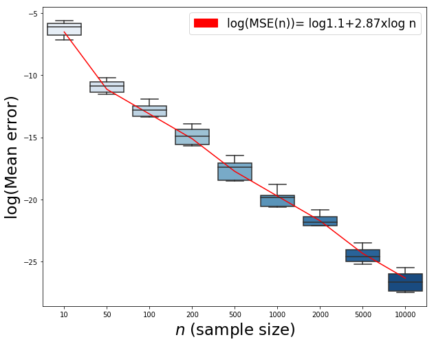
We consider different values for the sample size $n$ and for each of them we sample $100$ Gram matrices in the case $d=3$ and run the Algorithm 1 for each. We compute each time the mean squared error, defined by

In Figure 1 we put the $MSE_{n}$ for different values of $n$, showing how $MSE_{n}$ decrease in terms of $n$. For each $n$, the $MSE_{n}$ we plot is the mean over the $100$ sampled graphs.

We conducted a simulation study using graphon $W_{1}$, sampling $1000$ point on the sphere of dimension $d=3$ and we use Algorithm 1 to compute a score and recover $d$. We consider a set of candidates with $d_{max}=15$. In Figure 1 we provide a boxplot for the score of each candidate repeating the procedure $50$ times. We see that for this graphon, the algorithm can each time differentiates the true dimension from the “noise". We include more experiments in the supplementary material.

Invoke Theorem 12 with $Y=\hat{T}_{n}-T_{n}$, which by definition have independent centered entries (conditional to latent points $\{X_{i}\}_{i=1}^{n}$), to obtain

for $\alpha\in(0,1/3)$. Note that for $n$ large enough, one has

by Theorem 12, because $D_{0}=\max_{0\leq i\leq n}\sum^{n}_{j=1}\Theta_{ij}(1-\Theta_{ij})$ is $\mathcal{O}(n\rho_{n})$. Thus, for $n$ large enough we have

provided that $\frac{\sqrt{\log n}}{\rho_{n}n}=o(1)$, which is the case when $\rho_{n}=\Omega(\log n/n)$, which we have called the relatively sparse case. Let $V\in\mathbb{R}^{n\times d}$ and $\hat{V}\in\mathbb{R}^{n\times d}$ be two matrices with columns corresponding to the eigenvectors associated to eigenvalues $\lambda_{i_{1}},\lambda_{i_{2}},\ldots,\lambda_{i_{d}}$ and $\hat{\lambda}_{i_{1}},\hat{\lambda}_{i_{2}},\cdots,\hat{\lambda}_{i_{d}}$ of $T_{n}$ and $\hat{T}_{n}$ respectively, as in Theorem 13. We use Lemma 10 with $A=\hat{V}\hat{O}$ and $B=V$, where $\hat{O}$ is an orthogonal matrix, and Theorem 13 assuming that the right hand side of (9) is smaller than $1$, obtaining

where $\Delta:=dist(\{\lambda_{i_{1}},\cdots,\lambda_{i_{d}}\},\lambda(T_{n})\setminus\{\lambda_{i_{1}},\cdots,\lambda_{i_{d}}\})$. Then we have

Now, we use the $\delta_{2}$ metric to quantify the convergence of the eigenvalues of the normalized probability matrix $\frac{1}{\rho_{n}}T_{n}$ to the eigenvalues of the integral operator $T_{W}$. From Theorem 19 we have that, when $n$ is large enough

References

- [1] E. Arias-Castro, A. Channarond, B. Pelletier, and N. Verzelen. On the estimation of latent distances using graph distances. arXiv:1804.10611, 2018.
- [2] A. Bandeira and R. Van Handel. Sharp nonasymptotic bounds on the norm of random matrices with independent entries. Annals of Probability, 44(4):2479–2506, 2016.
- [3] R. Bathia. Matrix Analysis. Springer Verlag New York, 1997.
- [4] C. Borgs, J.T. Chayes, L. Lovasz, V.T Sos, and K. Vesztergombi. Convergent sequences of dense graphs i. subgraph frequencies,metric properties and testing. Adv. Math, 219(6):1801–1851, 2008.
- [5] C. Borgs, J.T Chayes, L. Lovasz, V.T. Sos, and K. Vesztergombi. Convergent sequences of dense graphs ii. multiway cuts and statistical physics. Annals of Mathematics, 176(1):151–219, 2012.
- [6] M. Braun. Spectral Properties of the Kernel Matrix and their Relation to Kernel Methods in Machine Learning. PhD thesis, Rheinische Friedrich-Wilhelms-Universität, Bonn, 2005.
- [7] S. Chatterjee. Matrix estimation by universal singular value thresholding. Annals of Statistics, 43(1):177–214, 2015.
- [8] F. Dai and Y. Xu. Approximation theory and harmonic Analysis on spheres and balls. Springer Verlag Monographs in Mathematics, 2013.
- [9] Y. De Castro, C. Lacour, and T.M. Pham Ngoc. Adaptive estimation of nonparametric geometric graphs. arxiv.org/pdf/1708.02107.
- [10] J. Diaz, C. McDiarmid, and D. Mitsche. Learning random points from geometric graphs or orderings. arXiv:1804.10611, 2018.
- [11] M. Emery, A. Nemirovski, and D. Voiculescu. Lectures on probability theory,. Springer-Verlag Berlin Heidelberg, Ecole d’ete de probabilites de saint-flour XXVIII edition, 1998.
- [12] P. Erdös and A. Rényi. On the evolution of random graphs. Publ. Math. Inst. Hungar. Acad. Sci, 5:17–60, 1960.
- [13] E.N. Gilbert. Random plane networks. J.Soc.Industrial Applied Mathematics, 9(5):533–543, 1961.
- [14] D.J. Higham, M. Rasajski, and N. Przulj. Fitting a geometric graph to a protein-protein interaction network. Bioinformatics, 24(8):1093–1099, 2008.
- [15] F. Hirsch and G. Lacombe. Elements of functional analysis. Springer-Verlag New York, 1999.
- [16] P. Hoff, A. Raftery, and M. Handcock. Latent space approaches to social network analysis. Journal of the American Statistical Association, 97(460):1090–1098, 2002.
- [17] R. Horn and C. Johnson. Matrix Analysis. Cambridge University Press, 2012.
- [18] X. Jia. Wireless networks and random geometric graphs. Proc. Int. Symp. Parallel Architectures, Algorithms and Networks, pages 575–579, 2004.
- [19] O. Klopp, A. Tsybakov, and N. Verzelen. Oracle inequalities for network models and sparse graphon estimation. Annals of Statistics, 45(1):316–354, 2017.
- [20] V. Koltchinskii. Asymptotics of spectral projections of some random matrices approximating integral operators. Progress in Probability, 43(In: Eberlein E., Hahn M., Talagrand M. (eds) High Dimensional Probability):191–227, 1998.
- [21] V. Koltchinskii and E. Giné. Random matrix approximation of spectra of integral operators. Bernoulli, pages 113–167, 2000.
- [22] K. Levin and V. Lyzinski. Laplacian eigenmaps from sparse, noisy similarity measurements. IEEE Transactions on Signal Processing, 65:1998–2003, 2017.
- [23] L. Lovasz. Large networks and graph limits. Colloquium Publications (AMS), 2012.
- [24] L. Lovász and B. Szegedy. Limits of dense graph sequences. J.Combin.Theory.Ser B, 96(6):197–215, 2006.
- [25] S. Nicaise. Jacobi polynomials, weighted Sobolev spaces and approximation results of some singularities. Math. Nachr., 213:117–140, 2000.
- [26] M Penrose. Random geometric graphs. Oxford University Press, first edition, 2003.
- [27] D.L. Sussman, M. Tang, and C.E. Priebe. Consistent latent position estimation and vertex classification for random dot product graphs. IEEE transactions on Pattern Analysis and Machine Intelligence, 36:48–57, 2014.
- [28] M Tang, D.L Sussman, and C.E Priebe. Universally consistent vertex classification for latent position graphs. Annals of Statistics, 41:1406–1430, 2013.
- [29] R. Vershynin. How close is the sample covariance matrix to the actual covariance matrix? Journal of Theoretical Probability, 25:655–686, 2012.
- [30] R. Vershynin. High-Dimensional Probability: An Introduction with Applications in Data Science. Cambridge University Press, 2018.
- [31] M. Walters. Random geometric graphs. Surveys in Combinatorics, pages 365–402, 2011.
- [32] Y. Yu, T. Wang, and R.J. Samworth. A useful variant of the Davis-Kahan theorem for statisticians. Biometrika, 102(2):315–323, 2015.
A Graphon regularity
One way to define the regularity of a geometric graphon on is through the notion of weighted Sobolev spaces on the interval . In that context, the regularity is related to the rate at which the eigenvalue sequence tends to . Here we follow [25]. For a function of the form , we define the norm
We will say that belongs to weighted Sobolev space if . We will refer to as the regularity parameter. As in the case of classical Sobolev spaces, there is a definition of weighted Sobolev spaces that involves the integrability (with respect to the measure ) of the weak derivatives of a function. Then a function belongs to if it has weak derivatives that are integrable with respect to the weighted norm in with weight . In [25] the authors prove that both definitions are in fact equivalent.
B Geometric Graphons have as the largest eigenvalue
To avoid border issues in Algorithm , we use the fact that the eigenvalue associated to the Gegenbauer polynomial for is the largest one, which in the notation of the paper can be written as . This is true for all geometric graphons.
Lemma 6.
If is such that
for , then
is constant.
Proof.
The proof follows from a change of variable. ∎
The following theorem is an analogous result to a classical theorem of spectral graph theory
Theorem 7.
For a graphon we have
By Courant-Fisher min-max principle we have
In particular, if we take the function for we have
the last follows form the definition of and the fact that is a probability measure on the sphere. On the other hand, if is an eigenfunction associated with we can choose such that for . Without loss of generality, assume that . So
which finish the proof ∎
C Proof of the rate of convergence of the Algorithm
This section is devoted to the proof of the main theorem, Theorem 2.2. In the sequel, the sentence “ large enough” means that is bigger than some that may depend on and . Recall that the result obtained will hold with probability with arbitrarily small. We used through the paper, the notation , where is random variable and a constant, to indicate that the inequality holds with probability bigger than .
The aim is to bound and we will split it into two terms as follows
where the matrix will be defined later (see Proposition 8) using a subset of eigenvectors of . We will treat these terms separately starting with in Section C.2 and the other term in Section C.3.
The first step is to control the probability of the following event
where is the spectral gap . We will prove in Section C.1 that this event holds with probability when is large enough. This event ensures that the “noise level” is lower than the spectral gap and it guarantees that our algorithm recovers the right subset of eigenvectors as will see in Proposition 8, Section C.1.
C.1 Event guaranteeing the algorithm convergence
Invoke Theorem 12 with , which by definition have independent centered entries (conditional to latent points ), to obtain
for . Note that for large enough, one has
by Theorem 12, because is . Thus, for large enough we have