Performance Analysis of OFDM with Peak Cancellation Under EVM and ACLR Restrictions

Figure 1 illustrates an E-SDM OFDM system model, where $M$, $N$, and $K$ denote the number of transmit antennas, receive antennas, and data streams, respectively. $\bm{W}_{t}^{l}$ and $\bm{W}_{r}^{l}$ denote precoding and post-coding matrices on the $l$-th subcarrier, respectively, where $l=1,\cdots,L$, and $L$ denotes the number of subcarriers. Here, the transmit data vector of the $l$-th subcarrier $\bm{x}^{l}=[x_{1}^{l},...,x_{k}^{l},...,x_{K}^{l}]^{T}$ is multiplexed by the precoding matrix $\bm{W}_{t}^{l}=[\bm{w}_{t1}^{l},...,\bm{w}_{tk}^{l},...\bm{w}_{tK}^{l}]$, where $\bm{w}_{tk}^{l}=[w_{tk1}^{l},...,w_{tkm}^{l},\dots,w_{tkM}^{l}]^{T}$ is the $l$-th column vector of $\bm{W_{t}^{l}}$ for the $k$-th data stream and superscript $T$ stands for transposed matrix. In E-SDM, left singular vector and right singular vector of the channel matrix are used as precoding and post-coding matrices, respectively. $\bm{H}^{l}$ stands for $N\times M$ matrix of the $l$-th subcarrier defined as

where $h_{nm}$ denotes impulse response of the path, Here, the $m$ and $n$ denote the transmit antenna index and the receive antenna index, respectively. Using with singular value decomposition (SVD), ${\bm{H}}^{l}$ can be decomposed into

where ${\bm{U}}_{l}$ and ${\bm{V}}_{l}^{H}$ are left and right singular vector of ${\bm{H}}^{l}$, and $(\cdot)^{H}$ means complex conjugate operation. $\Sigma_{l}={\rm diag}(\sqrt{\lambda_{1}^{l}},\sqrt{\lambda_{2}^{l}},...,\sqrt{\lambda_{M}^{l}})$ is a diagonal matrix and $\sqrt{\lambda_{m}^{l}}$ is the singular value of $m$-th stream. Transmit and receive spatial filter are defined as ${\bm{W}}_{t}^{l}={\bm{V}}_{l}$ and ${\bm{W}}_{r}^{l}={\bm{U}}_{l}^{H}$. The precoded QAM data stream is modulated with inverse fast Fourier transform (IFFT) and then PAPR reduction technique is applied at each transmits antenna. The guard interval (GI) is added to every symbol to remove inter-symbol interference. Perfect channel estimation is assumed.

After removing GI and carrying out FFT processing, the received signal is multiplied by the post coding matrix $\bm{W_{r}}^{l}=[\bm{w_{r1}}^{l},...,\bm{w_{rk}}^{l},...\bm{w_{rK}}^{l}]^{T}$, where $\bm{w}_{rn}^{l}=[w_{rn1}^{l},...,w_{rnk}^{l},...,w_{rnK}^{l}]^{T}$ denotes the $n$-th post-coding vector of the $l$-th subcarrier. Hence, the de-multiplexed signal vector $\bm{y}^{l}=[y_{1}^{l},...y_{k}^{l},...y_{K}^{l}]^{T}$ of the $l$-th subcarrier is given as

where ${\bm{U}}_{l}$ and ${\bm{V}}_{l}$ are unitary matrices and $\bm{n}^{l}=[n_{1},...n_{n},...,n_{N}]^{T}$ is an additive white Gaussian noise (AWGN) vector at each receive antenna.

In this paper, we evaluate the amount of OoB radiations as ACLR which is defined as

Here, $S_{t}=\frac{1}{2}E\left[|x^{l}_{k}|^{2}\right]$ denotes the average power of the transmit signal and $S(\omega)$ is the power spectral density of the transmitted signal. Let $f_{U}$- and $f_{L}$ denote the measured ACLR at an upper and lower band, respectively. The permissible maximum ACLR is set to $-50$ dB for transmitting signals at every antennas.

We also evaluate in-band distortion by measuring EVM which is defined as:

where $S_{t}[l]$ is the average power of the $l$-th subcarrier signal. $X_{l}$ and $\tilde{X}_{l}$ denote the complex signals at the $l$-th subcarrier (after FFT operation) without and with PAPR reduction, respectively. In E-SDM case, $X_{l}$ and $\hat{X}_{l}$ are defined as complex signals and replicated at the $l$-th subcarrier of each eigen-channel by Eq. (6).

Whenever the maximum signal amplitude exceeds a given threshold level $A_{th}$, the maximum peak is suppressed by adding a PC signal. Here, the PC signal is a scaled OFDM symbol whose subcarriers are added up to be in-phase at a given symbol time instant. The PC signal is generated by scaling the following basic function $g(t)$ as

where $p_{l}(t)$ is the transmit pulse at the $l$-th subcarrier. In this paper, we assume that $p_{l}(t)$ is the same rectangular pulse on all subcarriers whose amplitude is unity. The time-domain waveform of $g(t)$ is truncated by a windowing function $w(t)$; the truncated version of $g(t)$ is given as

We use the following windowing function to truncate the peak cancellation signal waveform:

where $0<T_{1}\leq T_{2}$. Here, $T_{1}$ is a design parameter to optimize distortions appeared after peak cancellation. $T_{2}$ denotes window size of $w(t)$. The truncated PC signal waveform and its frequency spectrum of $g^{\prime}(t)$ are illustrated in Figs. 3 (a) and (b), respectively. Here, parameters of windowing function are given as $(T_{1},T_{2})=(T/8,T/4)$. The PC signal explicitly exhibits high peak amplitude which is utilized to reduce the PAPR of OFDM.

In the proposed method, the optimum peak detection threshold should be selected so that the signal amplitude is suppressed below the threshold level, while EVM and ACLR are kept below the pre-defined values. This subsection describes the optimum threshold selection. Figure 4 illustrates an example of an OFDM signal waveform. In this figure, red and blue lines show the signal with and without the proposed peak cancellation, respectively. The green-shaded area corresponds to signal amplitude exceeding the peak detection threshold $A_{th}$. As illustrated in Fig. 4, adding the PC signal distorts the OFDM signal and increases both EVM and ACLR.

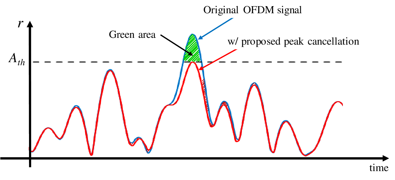
Figure 5 illustrates the relation between the scaling factor of the PC signal and the peak detection threshold, where $\zeta$ and $A_{th}$ denote the maximum amplitude of the OFDM signal and the peak detection threshold, respectively. As illustrated in Fig. 5, when the maximum amplitude $\zeta$ exceeds the threshold level $A_{th}$, OFDM signal amplitude is reduced to the threshold level by adding the PC signal whose amplitude is scaled to $\zeta-A_{th}$. Since the scaled PC signal is given as $(\zeta-A_{th})g^{\prime}(t)$, the energy of the scaled PC signal is calculated as

where $f_{in}$ and $f_{out}$ denote bandwidths to measure EVM and ACLR, respectively. Here, $G^{\prime}(\omega)=\int_{-\infty}^{\infty}g^{\prime}(t)e^{-j\omega t}dt$. $E_{i}$ and $E_{o}$ denote in-band power and out-of-band power of PC signal, respectively. Statistical distribution of instantaneous power of the OFDM signal follows exponential distribution as

where $\zeta^{2}$ and $S_{t}=\sigma^{2}$ denotes instantaneous power and average power of OFDM signal, respectively. Thus, the average signal distortion due to peak cancellation is calculated as

The in-band distortion power is given as

Assuming $E_{i}\gg E_{o}$, the normalized signal distortion is restricted as

where the average power of the signal is $S_{t}=\sigma^{2}$ and $\frac{e_{r}}{\sigma^{2}}$ denotes the pre-determined value of the maximum acceptable EVM. Hence, the minimum (optimum) peak detection threshold $A_{th}^{o}$ that meets the EVM requirement is given as

Here, $(A^{o}_{th})^{2}$ corresponds to the peak power of the OFDM signal after peak cancellation. Using Eq.(20), the optimum threshold $A^{o}_{th}$ to achieve pre-determined EVM value can be theoretically obtained.

In Fig. 2, the remaining three steps (i.e., “peak detection”, “distortion estimation”, and “PC signal scaling”) are repeated until the maximum value is below the threshold value unless ACLR or EVM exceeds their pre-defined values. At the first step, when the peak amplitude of the OFDM signal at $m$-th antenna exceeds the selected peak detection threshold at time instance $t=t_{0}$, the difference between the detected peak amplitude and the detection threshold, $A_{p}^{(m,i)}$, is calculated. In the next step, the increase of ACLR and EVM is estimated using the detected value $A_{p}^{(m,i)}$.

In multi-stream transmission in MIMO-OFDM, the peak cancellation is carried out to suppress the peak amplitude below the peak detection threshold under constraints of EVM and ACLR, where EVM and ACLR requirements are defined as an average value and the maximum value over all antennas, respectively.

Since the truncated signal $g^{\prime}[s]=g^{\prime}(s\Delta t)$ has out-of-band spectrum, it is clear that out-of-band radiation and in-band distortion appears by adding $g^{\prime}[s]$to the transmit signal, where $\Delta t$ denotes sampling interval. Here,

where $\mathcal{F}$ and $\ast$ denote discrete Fourier transform and convolution operator, respectively. $G[l]$ and $W[l]$ are frequency spectrum of the PC signal $g[s]$ and the window function $w[s]$, respectively.

Let $\Delta p_{o}$ and $\Delta p_{in}$ denote OoB signal power and in-band signal power of $g^{\prime}(t)$. Note that $\Delta p_{o}$ and $\Delta p_{in}$ are known values (calculated beforehand). Hence, when $G^{\prime}[l]$ is added to the signal to cancel the peak, the in-band distortion and OoB radiation are increased by

Let the total transmission power $S_{t}$ be constant, i.e., $S_{t}=\sum_{m=1}^{M}S^{(m)}$, where $S^{(m)}$ is the average signal power at the $m$-th transmit antenna. Let $|A_{p}^{(m,i)}|$ denote the difference between the threshold value and the $i$-th peak amplitude $x^{(i)}_{max}$ at the $m$-th antenna. EVM increase is expressed as $\displaystyle\frac{1}{S_{t}}|A_{p}^{(m,i)}|^{2}\Delta p_{in}$ when the PC signal is added to suppress the $i$-th peak amplitude $x^{(i)}_{max}$.

We calculate an average EVM value overall antennas as

where $\Delta p_{in}$ denotes the pre-determined constant. The averaged EVM value $\varepsilon_{e}^{(i)}$ is recursively calculated as

In order to restrict OoB radiation below the permissible value, we propose to estimate the instantaneous ACLR at each antenna as follows: When the $i$-th PC signal is added, the ACLR at each antenna is increased as

Using the above relation, the ACLR $\varepsilon_{a}^{(m,i)}$ after adding the $i$-th PC signal is recursively calculated as

Finally, the maximum value is calculated as

where $f(\cdot)_{max:m}$ is a function that selects the maximum value from possible ones with respect to antenna index $m$. From the practical design point of view Eq. (22) maybe used to directly calculate the level of degradation per subcarrier by simply reading out the signal amplitude level $A_{p}^{(m,i)}$ at the transmitter end.

The PC signal scaling and peak cancellation procedure in next step is done if both the average EVM $\varepsilon_{e}^{(i)}$ in Eq. (23) and the maximum ACLR ${\varepsilon_{a}^{(i)}}_{max}$ in Eq. (26) are less than the pre-defined levels.

To carry out the peak cancellation (i.e., the PC signal addition), both the averaged EVM values $\varepsilon_{e}^{(i)}$ and the estimated maximum ACLR ${\varepsilon_{a}^{(i)}}_{max}$ must be less than permissible values. Our proposed scheme can satisfy this condition automatically as explained below. First, when the maximum amplitude of the signal $x(t_{0})$ exceeds the threshold value, the scaled PC signal is expressed as

where $A_{p}=|x(t_{0})|-A_{th}$. $\theta_{0}$ is the phase of the signal $x(t_{0})$. Assume that the maximum amplitude exceeds the peak detection threshold at time instance $t^{(i)}_{0}$. Then, the amplitude of the OFDM signal after canceling the $i$-th peak amplitude is represented as

The above procedures are continued repeatedly until all amplitudes are suppressed below the peak detection threshold or the number of PC signal additions reaches a maximum number. However, if either the estimated ACLR or EVM exceeds the permissible value, the peak cancellation procedure stops before it reaches the maximum number. This stopping criterion guarantees that ACLR and EVM never exceed their permissible values.

In this section, first, we consider QPSK-OFDM signal whose subcarrier’s I and Q-phases take either $A$ or $-A$. Let $x_{e}$ denote a random variable which expresses signal distortion due to peak cancellation. Thus, the signal after peak cancellation is given as $\pm A+x_{e}$. We assume that $x_{e}$ follows Gaussian distribution with variance $\sigma_{e}^{2}$ and average value $\bar{x}_{e}$;

where $\sigma_{e}^{2}$ and $\bar{x}_{e}$ are variance and average amplitude of $x_{e}$. Since the average power of the signal is decreased after peak cancellation, it can be intuitively seen that $\bar{x}_{e}$ decreases as $A_{th}$ decreases, while $\sigma_{e}$ increase as $A_{th}$ decreases. Hence, the average value of $x_{e}$ can be expressed with $S_{in}$ as

where $L$ denotes the number of subcarriers. $\alpha$ is a constant depending on PC signal waveform $g^{\prime}(t)$ given as

where $f_{c}(x)$ denotes a clipping function defined as

The numerator and the denominator in Eq.(31) show integral of positive side PC signal amplitude and that of its absolute value, respectively. The variance of $x_{e}$ is given as

where $\mu=1-\bar{x}_{e}/A$. Here, $\langle x\rangle$ denotes expected value of the variable $x$.

Let $x_{n}$ denote additive white Gaussian noise (AWGN) with average level $A$ and variance $\sigma_{n}^{2}$, i.e., PDF of $x_{n}$ is given as

$x_{e}$ and $x_{n}$ are Independent and identically distributed (i.i.d.) random variables and therefore PDF of mixed variable $x=x_{e}+x_{n}$ is given as convolution of $p_{x}(x)$ and $p_{n}(x)$:

where $\beta$ denotes channel gain. BER for QPSK-OFDM signal after peak cancellation in AWGN condition with channel gain is expressed as

where $A$ denotes I and Q phase signal amplitudes.

The above discussion can be extended to multi-level QAM such as 16QAM and 64QAM. The same manner as QPSK case can be used for deriving BER expressions in QAM case except that variance of in-band noise is different, e.g., for 16QAM and 64QAM cases, their variances $\sigma_{e}^{16QAM}$ and $\sigma_{e}^{64QAM}$ are respectively given as

where $\sigma_{e}$ denotes variance in QPSK case. More generally, variance for $2^{Q}$ QAM is given as $\sigma_{e}/Q$

Figure 6 shows I-phase or Q-phase signal distribution of 16QAM at a certain subcarrier in the case with and without peak cancellation. Error probability of higher order bit $P_{eH}$ is given as a probability that signal $S_{1}$ and $S_{2}$ exceed threshold $T_{H}$;

Error probability of lower order bit of 16QAM is given as a probability that signal $S_{1}$ and $S_{2}$ exceed threshold $T_{L}$;

On the other hand, as illustrated in Fig.6(b), the average power of the signal and its distribution are reduced by peak cancellation.

Since it is clear that the optimum decision threshold for higher order bit is $T^{o}_{H}=0$, error probability of higher order bit is given as

Error probability of lower order bit of Gray-coded 16QAM using the optimum decision threshold $T^{o}_{L}$ in AWGN condition in the case with peak cancellation is

The optimum decision threshold $T^{o}_{L}=-2\mu\delta/\sqrt{\beta}$ to minimize BER can be derived by $\frac{\partial P_{eL}(T^{o}_{L})}{\partial T^{o}_{L}}=0$. Details of the derivation are given in the Appendix. Average BER is given by averaging Eq.(39) and Eq.(40).

In this subsection, we consider an Eigen-beam space division multiplexing (E-SDM) OFDM in $M\times N$ MIMO systems, where $M$ and $N$ denotes number of transmit antenna and the number of receive antennas, respectively. Hereafter, we assume $M=4$ and $N=2$ as an example. PDFs of eigen values with order for random $M\times N$ MIMO channel matrix are given as [11]:

where

Thus, BER expression of signal transmission over the $i$-th eigen channels in $M\times N$ MIMO channel can be derived as

where $M$ and $N$ denote the number of transmit and receive antennas. $p(\lambda,x)$ denotes PDF of the signal after peak cancellation in presence of AWGN and $\lambda_{i}$ is the $i$-th eigen vector. Similarly single antenna case, for QPSK transmission over $i$-th eigen channel,

Average BER over the first and second eigen channel is given as

where the same power is allocated to the first and the second eigen channels.

Figures 8(a) and (b) illustrate the statistical distribution of the normalized instantaneous signal power of transmitting signals in single-antenna OFDM and $4\times 2$ MIMO-OFDM, respectively. Here, we use CCDF to evaluate the statistical distribution and the instantaneous is normalized by average power of the signal. For comparison, CCDFs of cases of repeated C&F in [18][19] and other limiter based approaches in [31][32] are also shown. In repeated C&F [18][19], we note here that both ACLR and EVM satisfy the required values. In [32], $v$=7, $a$ = 0.05 and $A_{th}$ = 1 are used. In [31][32], roll-off filter with roll-off factor = 0 is used. Figure 8(a) shows that the instantaneous power of transmit signal with the proposed method is limited to around 5.12 dB and 7.25 dB at CCDF=$10^{-4}$ for QPSK and 64QAM data modulation schemes. The optimum threshold value is $P_{th}$=5.12 dB and 7.25 dB for QPSK and 64QAM data modulation schemes, respectively. Note that the achieved PAPR by the proposed method is close to the optimum threshold value. In other words, the threshold value corresponds to the achievable PAPR. As for comparison with other approaches, although methods in [31][32] show lower PAPR than the proposed method, it suffers from high in-band distortion which results in BER degradation as discussed in Fig. 12(b). Note that the proposed method is able to reduce the PAPR to a lower value compared to [31][32] if the required EVM value is set to a higher value, because the proposed method works to automatically minimize the peak power under given EVM and ACLR requirements. It can be also seen that instantaneous power in the case of repeated C&F is approaching the proposed method by increasing the number of iterations in the repeated C&F; almost the same CCDF in comparison with the proposed method is achieved with $N_{it}=9$. Similar findings are observed in Fig. 8(b) for E-SDM case.

Figures 9(a) and (b) illustrate the BER performance of single-antenna OFDM with the peak cancellation in AWGN channel, In this figure, peak cancellation is conducted under ACLR and EVM restrictions. Here, QPSK and 16QAM are used as subcarrier modulation. The BER curve of OFDM without any degradation due to peak cancellation is labeled as ”ideal case”. It is demonstrated in Fig. 10(a) that the proposed method achieves very close BER performance to ideal case, where EVM satisfies the pre-defined requirements $-20$ dB for QPSK and $-25$ dB for 16QAM, respectively. These figures also indicate that the theoretical BER curves show good agreements with its simulation results.

Figure 10 and  12 illustrate the BER performance of single-antenna OFDM and $4\times 2$ MIMO using eigen-mode in Rayleigh fading channel, respectively. Here QPSK and 16QAM are used as subcarrier modulation. EVM and ACLR are restricted below the pre-defined values, respectively. These figures also indicate that the theoretical BER curves show good agreements with their simulation results. It can also be seen from Fig. 12 that BER performance of the first and second streams in E-SDM scenarios show good agreements with their simulation results. We note here that EVM and ACLR meet the pre-defined values.

BER of the proposed method is compared with those of the conventional approaches in [18], [31] and [32] in Fig. 12, where QPSK and 16QAM are used for subcarrier modulation in Figs. 12(a) and Fig. 12(b), respectively. The Purple line shows the BER of the repeated C&F [18] using the same threshold as the proposed peak cancellation. The blue line and the green line show the BER of the repeated C&F in [31] and that of the companding technique in [32], respectively. Here, parameters in the repeated C&F and companding are same in Fig. 8(a). The red line shows the BER of the proposed method. In Fig. 12, for QPSK case, it can be seen that the proposed method and conventional methods in [18][31] show almost the same BER. On the other hand, for 16QAM case, BER of the conventional methods are significantly degraded, while the proposed method shows good BER performance comparable to the ideal case. This is because the proposed method is able to keep EVM below the predefined threshold automatically unlike the conventional methods.

This subsection evaluates a computational complexity of required PAPR reduction procedures between the two methods above. In this comparison, the number of complex multiplications is used as the complexity metric. When PC signal is added $N_{pc}$ times per OFDM symbol, the complexity of the proposed method is $\left\langle N_{w}\times N_{pc}\right\rangle$, where $N_{w}$ denotes the number of complex multiplications per PC addition. On the other hand, the complexity of the C&F with time domain LPF is given as $\left\langle\sum_{j=1}^{N_{it}}(N_{tap}\times N^{(j)}_{th})\right\rangle$. Here, $\left<x\right>$ denotes the averaging of $x$. $N_{it}$ and $N_{tap}$ denote the number of iterations and the number of taps in time domain filter, respectively. $N^{(j)}_{th}$ is the number of samples exceeding a given threshold per OFDM symbol. $j$ denotes the iteration index.

The required complexity for the peak cancellation in SDM-OFDM is evaluated in comparison with the repeated C&F based on the above defined metric in Fig. 13 where $M=4$ and $N=2$ are assumed. In the figure, we assume QPSK is adopted as subcarrier modulation. Here, PAPR is defined as the normalized instantaneous power observed at CCDF=$10^{-4}$. The red line shows the result of the proposed method, while the results of repeated C&F method are depicted by other color lines. The color-fill circular shape markers represent that both EVM and ACLR requirements are fulfilled, while the white-fill shows that either EVM or ACLR (or both) exceed the pre-defined value. In repeated C&F cases, normalized instantaneous power is approaching the peak detection threshold $S_{th}=10\log_{10}\frac{A^{2}_{th}}{S_{t}}$ by repeating clipping and filtering operations. Note that in the proposed method, ACLR and EVM can be kept below the required values automatically, unlike the repeated C&F method. This figure proves that the required complexity for the proposed peak cancellation is lower in comparison with the repeated C&F.

Figure 14 illustrates the relationship between the required complexity and achievable ACLR as a function of window size truncating the PC signal in terms of required EVM values which are set to $-20$, $-25$ or $-30$ dB, where red drawn circle markers denote selected window size for each EVM value in case of ACLR$=-50$ dB. The threshold is selected to meet the required EVM as discussed in Sect. IV and correspond to achievable PAPR and BER. The PC signal is truncated by the window function $w(t)$ as shown by Eqs. (9)-(IV), Thus, window-size $T_{2}$ affects both ACLR and the complexity. It can be seen that from this figure as window-size increases, ACLR decreases at the expense of increasing the required complexity. The results suggest that the required complexity is minimized by optimizing the window-size under a given EVM (i.e., BER) and threshold value (i.e., PAPR).

References

- [1] T. Hwang, C. Yang, G. Wu, S. Li, and G. Ye Li, “OFDM and Its Wireless Applications: A Survey,” IEEE Trans. Vehic. Tech., Vol.58, No.4, pp.1673-1694, May 2009.
- [2] Y. Akaiwa, “Introduction to Digital Mobile Communication, 2nd Edition,” Wiley, June 2015.
- [3] S.H.Han and J.H.Lee, “An Overview of Peak-to-Average Power Ratio Reduction Techniques for Multicarrier Transmission, ” IEEE Wireless Communications, pp.57-65, April 2005.
- [4] Y. Rahmatallah and S. Mohan, “Peak-To-Average Power Ratio Reduction in OFDM Systems: A Survey And Taxonomy,” IEEE Commun. Surveys & Tutorials, vol.15, no.4, pp.1567-1592, 2013.
- [5] R. W. Baüml, R.F. H. Fischer and J. B. Huber, “Reducing the peak-to-average power ratio of multicarrier modulation by selected mapping,” Electron. Lett., vol.32, no.22, pp.2056-2057, Oct. 1996.
- [6] D.-W. Lim, J.-S. No, C.-W. Lim, and H. Chung, “ A New SLM OFDM Scheme With Low Complexity for PAPR Reduction,” IEEE Signal Processing Letters, Vol. 12, No. 2, Feb. 2005.
- [7] S. H. Müller and J. B. Huber, “OFDM with reduced peak-to-average power ratio by optimum combination of partial transmit sequence,” Electron. Lett., vol.33, no.5, pp.368-369, Feb. 1997.
- [8] L. J. Cimini and N. R. Sollenberger, “Peak-to-Average Power ratio reduction of an OFDM signal using partial transmit sequence,” IEEE Commun. Lett., vol.4, no.3, pp.86-88, March 2000.
- [9] O. Muta and Y. Akaiwa, “Weighting Factor Estimation Method for Peak Power Reduction Based on Adaptive Flipping of Parity Bits in Turbo-Coded OFDM Systems,” IEEE Trans. Vehicular Technology, vol.57, no.6, Nov. 2008.
- [10] O. Muta, “Construction and Blind Estimation of Phase Sequences for Subcarrier-phase Control Based PAPR Reduction in LDPC-Coded OFDM Systems,” IEICE Trans. Fundamentals, vol.E93-A, no.11, Nov. 2010.
- [11] J. Tellado and J. M. Cioffi, “Efficient algorithms for reducing PAR in multicarrier systems,” IEEE International Symposium on Information Theory, p. 191, Aug. 1998.
- [12] P. Boonsrimuang, K. Mori, T. Paungma, and H. Kobayashi, “Proposal of Simple PAPR Reduction Method for OFDM Signal by Using Dummy Sub-Carriers,” IEICE Trans. Commun., vol.E91.B, no.3, pp.784-794, March 2010.
- [13] B. S. Krongold and D. L. Jones, “PAR Reduction in OFDM via Active Constellation Extension,” IEEE Trans. Broadcast., vol. 49, no. 3, pp. 258-268, Sept. 2003.
- [14] T. A. Wilkinson, and A. E. Jones, “Minimization of the peak to mean envelope power ratio of multicarrier transmission schemes by block coding,” in Proc. IEEE Vehicular technology Conf., pp.825-829, 1995.
- [15] A. E. Jones and T. A. Wilkinson, “Combined coding for error control and increased robustness to system nonlinearities in OFDM,” in Proc. IEEE Vehicular technology Conf., pp.904-908, 1996.
- [16] S. Shepherd, J. Orriss, and S. Barton, “Asymptotic limits in peak envelope power reduction by redundant coding in orthogonal frequency-division multiplex modulation,” IEEE Trans. Commun., vol.45, no.1, pp.5-10, Jan. 1998.
- [17] X. Li and L. J. Cimini, ”Effect of clipping and filtering on the performance of OFDM,” IEEE Commun. Lett., vol.2, no.5, pp.131-133, May 1998.
- [18] J. Armstrong, Peak-to-average power reduction for OFDM by repeated clipping and frequency domain filtering,” Electron. Letters, vol.38. no.5, pp.246-247, Feb. 2002.
- [19] S. Tomisato and H. Suzuki, “A peak reduction scheme based on control signal insertion for multi-carrier mobile communication,” IEICE Trans. Commun., vol. E86-B, no.6, pp. 1910-1916, June 2003.
- [20] M. M. Lee and Y. Kim, “An adaptive clipping and filtering technique for PAPR reduction in OFDM systems,” Circuits Syst. Signal Process. Vol.32, no.3, pp.1335-1349, Jun. 2013.
- [21] M. Pauli and H.-P. Kuchenbecker, “Minimization of the Intermodulation Distortion of a Nonlinearly Amplified OFDM Signal,” Wireless Personal Commun., Vol.4 pp.93-101, 1996.
- [22] X. Huang, J. Lu, J. Zheng, K. B. Letaief, and J. Gu, “Companding transform for reduction in peak-to-average power ratio of OFDM signals,” IEEE Trans. Wireless Commun., vol. 3, Issue 6, pp. 2030-2039, Nov. 2004.
- [23] T. Jiang, Y. Yang, and Y. Song, “Exponential companding technique for PAPR reduction in OFDM systems,” IEEE Trans. Broadcasting, vol.51, no.2, pp.244-248, June 2005.
- [24] L. Dan, T. Li, Y. Xiao, and S. Li, “Performance of peak cancellation for PAPR reduction in OFDM system,” International Conference on Communications, Circuits and Systems, 2008.
- [25] Y. Huang, “A Simplified Peak Cancellation Method for OFDM Signals,” International Conference on Computer Science and Electronics Engineering ICCSEE, 2012.
- [26] T. Hino, O. Muta, and H. Furukawa, “A Study on Peak Amplitude Suppression of OFDM Signals under Restriction of Out-of-Band Radiation Power,” The Transactions of IEICE B, Vol.J97-B, No.6, Jun. 2014 (in Japanese).
- [27] T. Kageyama, O. Muta, and H. Gacanin “An Adaptive Peak Cancellation Method for Linear-Precoded MIMO-OFDM Signals,” Proc. PIMRC’15, Sept. 2015.
- [28] Y.-C. Wang and A.-Q. Luo, “Optimized iterative clipping and filtering for PAPR reduction of OFDM signals,” IEEE Trans. Commun., vol. 59, no. 1, pp. 33-37, Jan. 2011.
- [29] X. Zhu, W. Pan, H. Li and Y. Tang, “Simplified approach to optimized iterative clipping and filter for PAPR reduction of OFDM signals,” IEEE Trans. Commun., vol.61, no.5, pp.1891-1901, May. 2013.
- [30] I. Sohn and S. C. Kim, “Neural network based simplified clipping and filtering technique for PAPR reduction of OFDM signals,” IEEE Commun. Lett., vol.19, no.8, pp.1438-1441, Aug. 2015.
- [31] K. Anoh, C. Tanriover, B. Adebisi and M. Hammoudeh, “A new approach to iterative clipping and filtering PAPR reduction scheme for OFDM systems,” IEEE Access, vol.6, pp.17533-17544, Sept. 2017.
- [32] B. Adebisi, K. Anoh and K. M. Rabie, “Enhanced nonlinear companding scheme for reducing PAPR of OFDM systems,” IEEE Systems journal, vol.13, issue 1, Mar. 2019.