Monotone smoothing splines with bounds
Abstract.
The problem of monotone smoothing splines with bounds is formulated as a constrained minimization problem of the calculus of variations. Existence and uniqueness of solutions of this problem is proved, as well as the equivalence of it to a finite dimensional but nonlinear optimization problem. A new algorithm for computing the solution which is a spline curve, using a branch and bound technique, is presented. The method is applied to examples in neuroscience and for fitting cumulative distribution functions from data.
1. Introduction
Splines and smoothing splines have a long history of application in many fields. The basic history is outlined in Egerstedt and Martin, [3] and in Wahba, [19]. See also [20] for an introduction to the use of smoothing splines in statistics. In this paper we return to the problem of monotone smoothing splines, which was previously studied in [3, 4, 8, 9]. A classical application is to determine the average growth curve of a population of juveniles. Suppose we have a population of perhaps 30 children whose heights are measured every 6 months from age 2 to 20. It is easy to fit a smoothing spline to the data set but there is no guarantee of monotonicity. Since people just do not get shorter and then regrow, the smoothing spline is not appropriate for this and other similar situations. Instead, the appropriate tool is the monotone smoothing spline. Charles, Sun and Martin [2] used monotone smoothing splines in calculating distribution functions. There a problem can arise in that the spline may become greater than at some point and by monotonicity it can never decrease, and so this violates the condition that a cumulative distribution only takes values between and , a problem that was not addressed in [2]. In this paper, we solve this problem by imposing a condition that the spline is bounded above by some number (which would be in the case of cumulative distribution functions). We also present an application of monotone smoothing splines in mathematical biology,where sigmoidally shaped function commonly occur.
The main difficulty of the problem is the monotonicity constraint , which has to hold at every point in the interval under consideration. This infinite dimensional constraint is handled by a vector space version of the Karush–Kuhn–Tucker theorem, and using this, it is possible to reduce the original infinite dimensional problem to a finite dimensional problem which can be solved numerically.
The paper is organized as follows: In Section 2, we formulate the curve fitting problem as a constrained Calculus of Variations problem, and in Section 3, we show existence and uniqueness of the minimizer of this minimization problem, and hence existence and uniqueness of the monotone smoothing spline function. In Section 4, we formulate the Karush–Kuhn–Tucker conditions for this problem, and use these to prove a key lemma, saying that the second derivative of is essentially piecewise linear. In Section 5, we use the key lemma from Section 4 to reformulate the infinite dimensional linear problem of Section 2 into a finite dimensional but nonlinear problem. This was essentially done previously in [3], except that we provide more details in the proof. We also introduce a new branch and bound type algorithm for computing the optimal curve. Sections 6 and 7 contain applications and examples which show how the method can be used. In Section 6, we reconstruct sigmoidal shaped curves arising in an intracellular signalling model, while in Section 7, we apply the method on reconstructing cumulative distribution functions using data, and in particular for a cumulative distribution function arising in the cell cycle, and the distribution that we reconstruct gives the time certain cells remain in a particular phase in the cell cycle.
2. The problem
Let , and let . Consider a data set with , with associated weights , .
Let , and consider the following optimization problem for functions defined on an interval :
| (1) |
subject to
| (2) |
where is the Sobolev space of twice weakly differentiable functions on . The condition is included because in many situations in applications, it is for modelling purposes clear that the curve must satisfy this condition. This happens for example in the application of the intracellular signalling model that we discuss in Section 6. The condition arises from . Since the curve is monotonically increasing, it suffices to impose the condition at the endpoint .
As is a bounded interval, we can use as a norm on . The rest of the paper is devoted to solving this problem, and to applications of the developed method.
3. Existence and uniqueness of a minimizer
Theorem 1.
Let , and assume that . There exists a unique which solves the minimization problem
Proof.
Let
| (3) |
We will use the direct method in the calculus of variations, which says that if a functional is coercive on and weakly lower semicontinuous on a weakly closed set, then a minimizer exists (see e.g. [17], p. 4). It is easy to see that the set is convex and closed in and hence it is weakly closed by Mazur’s lemma (see e.g. Theorem 3.13 of [12]).
We will first check that the first term of is weakly lower semicontinuous and coercive on . Indeed, it is weakly lower semicontinuous since
and so if (i.e. converges weakly to in ), then
i.e.
which shows that is weakly lower semicontinuous on . Coerciveness of the first term on is obvious since it is the square of the norm on .
Weak lower semicontinuity of the second term of (1) follows since is compactly embedded in . Indeed, if in , then is bounded in , and since the embedding of into is compact, has a subsequence , which converges (to by uniqueness of a weak limit) in ). Finally, note that for each ,
if in , and so the sum in (1) is weakly continuous.
As is a sum of two weakly lower semicontinuous functions, it is clear that is weakly lower semicontinuous on .
Next, we prove that is coercive on . As is coercive on , we see that
as .
To show uniqueness, we will show that is strictly convex. For this, we will use that and are strictly convex on and on , respectively. Let , , and , so that on . It is clear that , and are convex (but not strictly convex) functions on . To show that is strictly convex, we need to prove that if
| (4) |
for some and , , then .
To prove this, we assume that (4) holds. Since are convex for and , equation (4) holds also when is replaced by , . Since is strictly convex, the equality (4) for implies that . Then, by integration and using that , it follows that there exists a real constant such that .
On the other hand, since is strictly convex and , equality (4) for implies that . Combining this with , we obtain (since and ). We have proved that for all , and hence in . This concludes the proof that is strictly convex on , and from this it also follows that the minimizer is unique. ∎
4. The Karush–Kuhn–Tucker conditions
The constrained optimization problem will be solved with a vector space version of the KKT method, cf. Theorem 1 p. 249 of [6].
Let , and let , with a norm defined by
We define by
We note that since , it follows that , and so it is clear that .
It is straight-forward to check that is Fréchet differentiable, and its derivative is
By the Riesz representation theorem (see e.g. pp. 113–115 of [6], and pp. 146–150 of [18]), the dual space of is identified with the normalized space of functions of bounded variation on , denoted by , consisting of functions of bounded variation on such that is right-continuous and , such that the functionals on can be expressed as the Riemann–Stieltjes integral
and the norm of is the total variation of on , denoted by .
We denote the dual space of by . By the above result, is identified with , and the norm of an element is given by
The positive cone in is
It is clear that has a nonempty interior. The positive cone in is
We will derive the KKT conditions for the optimization problem of equation (1). In order to do this, we first show that all points satisfying the inequality (i.e. ) are regular points for this inequality (cf. [6], p. 248).
Lemma 1.
Every with is a regular point of the inequality .
Proof.
Let be such that . We need to show that there exists an such that is an interior point of , i.e. that satisfies
There are clearly many choices for , for example
With this choice, we have and
i.e. is an interior point of . ∎
The functional defined by (3) is Fréchet differentiable, and its derivative is given by
Let be the minimizer of subject to . By the KKT Theorem (see [6], p. 249), there exists a , (i.e. ) such that the Lagrangian
is stationary at , and that .
An explicit statement of the KKT conditions implies the following result, which will be used in the next section for constructing a numerical algorithm for the solution:
Lemma 2.
Remark 1.
We cannot conclude directly from Lemma 2 that is piecewise linear, since we cannot yet rule out that there is an increasing sequence of points such that while for (and is affine on each of the intervals ). We will see in Lemma 3, that this does not happen for the optimal curve, and is in fact piecewise linear.
Proof.
By the KKT conditions [6], p. 249, there exists a and a such that
| (5) |
for all . Furthermore,
| (6) |
where is nondecreasing and . Equation (6) is the complementary slackness condition, and together with the constraint , it implies that is constant for such that , and that if .
The Riemann-Stieltjes integral in (5) may be integrated by parts, and doing so and noting that (since and hence absolutely continuous), we obtain after collecting the two integral terms
| (7) |
for all . Choosing on all except one of the subintervals , , we conclude that for each ,
for all . Hence there exist , , such that on . We may assume (by choosing a representative for the function ), that on the half open interval for . Hence is a right continuous function of bounded variation.
Now with a general , the integral term of (7) can be rewritten using integration by parts as
By choosing appropriately (i.e. exactly one of and not equal to zero), we conclude that
| (8) | ||||
where we have also used that . In particular, since and , it follows that . Hence . Note that the first equation of (8) implies that is continuous at the spline knots , , and the second equation implies that the derivative of has jumps of size at , .
Recall that is (locally) constant for such that . Let us examine what happens for a point such that . If is an isolated zero of , then may have a jump discontinuity at (where it is right continuous). If on an interval around , then clearly also on this interval. In particular is piecewise linear in this interval. ∎
5. An algorithm for computing the optimal solution
Using Lemma 2, we will now reformulate the optimization problem as a finite dimensional problem which we can solve numerically. This is essentially the approach of Section 7.3 of [3], and their method has been adapted to the extra constraint . Instead of using dynamical programming as in [3], we give an outline of a branch and bound algorithm for finding an optimal solution to the problem. The variables of this new problem are , which are the (unknown) values of the function and its derivative at the spline knots.
Assuming initially that the values and are known, we will use the method of [3] to determine a curve with minimal cost under the constraint that it passes through the points with derivatives at these points equal to , respectively. This will give us a new cost function depending on the variables and . Minimizing this function is equivalent to the original infinite dimensional problem.
Now we focus our attention on one interval , and rename it . Without loss of generality, we assume that . The corresponding values of at the endpoints and are denoted by and , respectively. We assume without loss of generality that . The values of the derivatives at the endpoints are denoted by and . The following lemma is essentially given in [3], but here we provide the full proof with more details, taking care of excluding the pathological case in the remark after Lemma 2. Note also that a typo in formula (7.27) of [3] has been corrected ( instead of ).
Lemma 3.
[3] Suppose that , and . Then the optimal control which minimizes subject to the constraints for , , , , and for is given by
if , and
if . The contribution to the cost in the two cases is
The corresponding spline function is given by
if , and
| (9) |
if .
Proof.
The optimal control which minimizes subject to the constraints , , , , (that is all the constraints except the monotonicity constraint ), is an affine function where and are chosen so that the constraints are satisfied. This gives the expression
for all choices of , , and . By integration and using the remaining constraints, the corresponding curve on the interval is given by
Clearly, in the cases when the monotonicity constraint is satisfied, this curve is optimal also for the original problem. We claim that the on if and only if . To prove this, note that the quadratic function is given by
We note that and by the assumptions, and so for all if and only if the value of at an interior minimizer is nonnegative.
We study the cases and separately. If , then doesn’t have a minimizer, and so the monotonicity condition will always be satisfied. We note that in this case,
is always satisfied.
If , i e if , then we need a necessary and sufficient condition for when the minimum value of is nonnegative and the minimizer belongs to the interval . The minimizer belongs to the interval if and only if , i e if
which holds if and only if
| (10) |
The minimum value is nonnegative if and only if i e
and this inequality holds if and only if
We note that the right inequality is always satisfied if the minimizer belongs to the interval , by (10) and since . To summarize, we see that irrespective of the sign of , a necessary and sufficient condition for the monotonicity of on is that
as required. ∎
Let
In view of Lemma 2 and by considering functions which on each subinterval is of the form of Lemma 3, we have proved the following:
Theorem 2.
The infinite dimensional optimization problem of Section 2 is equivalent to the finite dimensional problem
| (11) |
subject to the constraints
The nonlinear optimization problem of Theorem 2 can be solved numerically, for example with fmincon in matlab. Unfortunately, this method does not seem to give stable results when there are more than 10 subintervals, and it is hard to analyse due to the piecewise defined objective function.
To come around this problem, we suggest using a branch-and-bound approach which is outlined below. We emphasise that the algorithm is guaranteed to terminate, since there are finitely many (at most , but probably much less in practice) subproblems to solve, each of which are convex and can be solved within a fixed time, e.g. with Newton’s method. We suggest that a breadth first search is used when going through the branches of the tree, and it is likely that for most problems it will not be needed to search through so many levels of the tree. Further investigations will be needed to find out how efficient the algorithm is and the limit of the size of the problem that can be solved in practice. These questions will be addressed in a future project. In the current paper (Sections 6 and 7) we give some examples where the method has been implemented for up to 30 data points with good results.
- 1.
Start by fitting an ordinary cubic smoothing spline using the data points and with the constraints that and . If this curve satisfies for every , or, equivalently for every , then this must be the optimal curve, and we can stop. Otherwise, the value of the optimal function for this step gives a lower bound for the optimal solution.
- 2.
If the curve in step 1 was not optimal, we branch the problem into subproblems, where each subproblem corresponds to an interval for which the spline is given by a piecewise defined curve as in (9), whereas the spline should be an ordinary cubic spline on the other subintervals. A minimization problem is solved using (11), except that the first line in the definition is taken for the subintervals where the curve should be an ordinary spline, and the second line for the subinterval where the spline should be piecewise defined. The optimal value for each of these subproblems give lower bounds for the optimum of that branch. If the curve is monotone, then we have an optimum for the current branch and don’t need to branch any further. Otherwise, that node have to be branched into further subproblems, each with one more subinterval where we use a piecewise defined spline curve.
- 3.
We continue branching and bounding. Branches whose lower bound is smaller than an optimum in another side branch can be cut off, and don’t need to be examined further. In the end, we compare the branch with the smallest optimum, which will give the minimum of the full problem.
6. Applications to an intracellular signaling model
As a first application of the algorithm developed in Section 5, we suggest curve fitting using monotone smoothing splines as an alternative to the parametric models that are commonly used in modelling of pathways of the cell. This is expected to be particularly useful in cases where the underlying chemistry is not completely understood, but when certain monotonicity trends in the data can be observed. The ODE models or stochastic models that are commonly used can be very complicated, see e.g. [10] where the modelling process of this type of models is described. In Section 3 of this reference, a relatively simple modelling example of this type, occuring in neuroscience is given, which we describe briefly here, to give the reader context.
Calmodulin is an abbreviation for calcium-modulated protein, which is an intermediate calcium-binding messenger protein present in all eukaryotic cells. Once bound to a calcium ion, calmodulin acts as part of a calcium signal pathway by modifying its interactions with various target proteins such as kinases or phosphatases. Its importance in neuroscience stems from its crucial involvement in synaptic plasticity.
We consider five data sets with experimental data taken from [1, 11, 15, 16], corresponding to models describing this particular pathway. See [10, 5] for a model using a system of ordinary differential equations stemming from steady state equations for these reactions, and where the same data sets are used. This particular model consists of the elementary species calcium (Ca), calmodulin (CaM), protein phosphatase 2B (PP2B), and Ca/CaM-dependent protein kinase II (CaMKII) and protein phosphatase 1 (PP1).
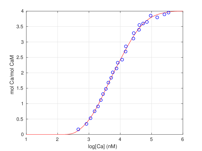
Up to four Ca ions are bound by calmodulin, and the first data set that we consider describes how many (moles of) ions of calcium are bound to CaM per (mole of) CaM, and this quantity is plotted versus the Ca concentration. When the Ca concentration increases, more Calcium ions are bound to the proteins, and it is therefore natural to assume that the curve corresponds to the graph of an increasing function. Each calmodulin molecule can bind at most four Ca ions, and hence the range of the function is naturally included in . When there is no Ca present in the system, there cannot be any bounds, and so we require that the curve passes through the origin. The data set is taken from [16], and the data together with the fitted monotone spline is shown in the first subfigure of Figure 1.
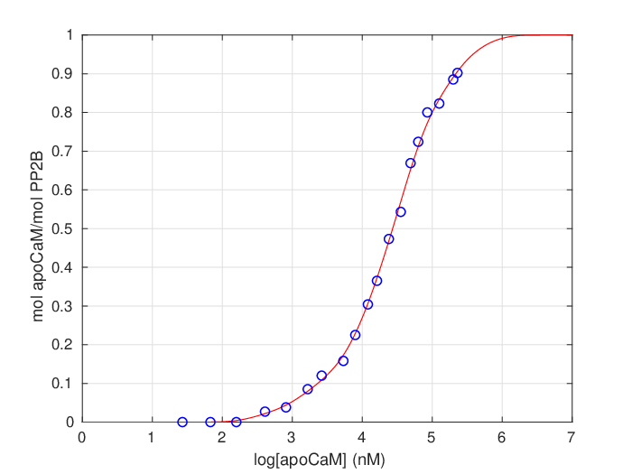
The binding of Ca ions by Calmodulin is a cooperative process. Ca-bound CaM activates PP2B, another protein implicated in molecular processes related to learning which also plays a role in striatal signaling. Dataset 2, which is taken from [11], describes the number of moles of apo calmodulin (apoCaM, i e calmodulin without calcium bound to it) bound to each mole PP2B versus the concentration of apoCaM. Since one PP2B molecule can bind at most one calmodulin molecule, the range of the function is naturally between and . As there has to be apoCaM in the system for this type of binding to occur, we require that the is on the curve. The more apoCaM there is in the system, the more likely it is for such a binding to occur, and it is hence natural to assume that the fitted function is increasing.
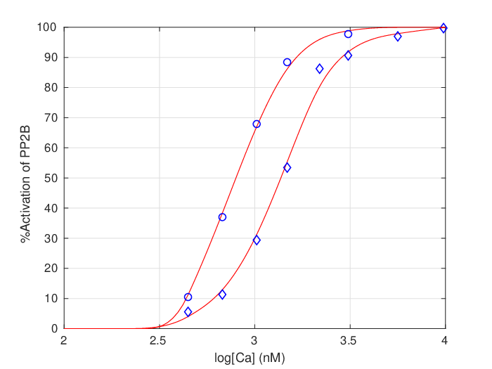
In the third subfigure, percentage activation of PP2B is plotted versus Ca concentration at two different concentrations of CaM (30 nM for the left curve and 300 nM for the right curve). The data for this subfigure is taken from [16]. Naturally, the range of the function is contained in , and the data suggests that the binding is more likely to occur for higher concentrations of Ca, and hence it is natural to fit the data with a curve which is the graph of an increasing function. Again, Ca is needed for the activation to occur, and for this reason we require that the curve starts at the origin.
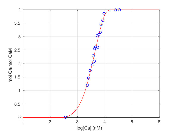
The third protein CaMKII, is a kinase, which is activated by the binding of Ca–CaM. In the fourth subfigure, we consider data from [15], representing the number of moles of Ca that is bound to CaM per mole of CaM in the presence of the enzyme CaMKII. As in subfigure 1, the curve is expected to be the graph of a function which is increasing, whose range is contained in , and which is originating from the origin.
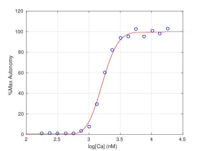
CaMKII molecules exist as dodecamers, consisting of two hexamer rings. A CaMKII unit that has bound CaM can autophosphorylate when sitting beside an active neighboring unit in the same hexamer ring. The phosphorylated unit can remain active even in the absence of Ca-CaM. In subfigure 5, the data comes from [1], and it describes the percentage phosphorylated CaMKII (autonomy in CaMKII activity) versus calcium concentration.
The method of the current paper is applied to data sets in order to fit curves which come close to the data points. The weights were set to for all examples and the parameter was chosen to be for the first two datasets and for the three last.
The same range was used for the variables as in Figure 12.3 of [10]. Instead of imposing a new type of condition corresponding to the limit as the independent variable tends to infinity, an additional data point was introduced, which forces the curve to come close to the maximum bound at the right endpoint of the interval. For example, for dataset 1, we demand that the curve comes close to the point . After doing this, the method of Section 5 could be used directly. The plots of Figure 1 were obtained, and these can be compared to the first five plots in Figure 12.3 of [10].
7. Applications for cumulative distribution functions and an example from cell cycle models
A second application to the technique of this paper, is for reconstructing an unknown distribution function given some data points.
Suppose that it is known that a sample comes from a distribution with an absolutely continuous distribution function, but that the exact form of the distribution is unknown. Then we could reconstruct the cumulative distribution function by using monotone splines. We first test the method from a sample of data points coming from a normal distribution.
Using , random points were generated following the normal distribution with expectation value and standard deviation . Then a histogram with bins was created using Matlab’s function histcounts. The vector with data values was created by using Matlab’s function cumsum. With , the method of this paper was used with the minor modification that is replaced by to create an approximation of the cumulative distribution function. By differentiating the obtained spline function an estimate for the density function could also be obtained. The results can be seen in Figure 2.


The method is more useful when the data does not come from a standard distribution, and the following is an example of such a situation arising in cell biology. The cell cycle consists of four distinct phases: , , and . For many types of cells, the time a cell spends in the phase is highly variable, and it is of interest to find the distribution for the time a cell spends in the phase. See for example [7], where such a distribution is used in an age structured cell cycle model. FUCCI is a fluorescence technology that can be used for tracking the time an individual cell spends in the phase [13, 14]. Using the movie S1 of the supplementary material of [13], the histogram data for the time that each cell in that movie stays in the phase was obtained. Using , the cumulative distribution function could be estimated and is shown in Figure 3


8. Acknowledgements
The author would like to thank Clyde Martin for reading and commenting on an earlier version of the manuscript and Olivia Eriksson for a useful discussion about the data sets occurring in Figure 1. She is also thankful to the reviewers for useful comments which led to an improvement of the paper.
References
- [1] Bradshaw, M., Kubota, Y., Meyer, T., and Schulman, H. An ultrasensitive ca2+/calmodulin-dependent protein kinase ii-protein phosphatase 1 switch facilitates specificity in postsynaptic calcium signaling. Proceedings of the National Academy of Sciences 100, 18 (2003), 10512–10517.
- [2] Charles, J., Sun, S., and Martin, C. Cumulative distribution estimation via control theoretic smoothing splines. In Three Decades of Progress in Control Sciences, X. Hu, U. Jönsson, B. Wahlberg, and B. Ghosh, Eds. Springer Berlin Heidelberg, 2010, ch. 7, pp. 95–104.
- [3] Egerstedt, M., and Martin, C. Control Theoretic Splines. Princeton University Press, Princeton and Oxford, 2010.
- [4] Elfving, T., and Andersson, L.-E. An algorithm for computing constrained smoothing spline functions. Numer. Math. 52, 5 (1988), 583–595.
- [5] Eriksson, O., Jauhiainen, A., Maad Sasane, S., Kramer, A., Nair, A., Sartorius, C., and Hellgren Kotaleski, J. Uncertainty quantification, propagation and characterization by bayesian analysis combined with global sensitivity analysis applied to dynamical intracellular pathway models. Bioinformatics 35, 2 (2019), 284–292.
- [6] Luenberger, D. G. Optimization by vector space methods. John Wiley & Sons, Inc. New York, London, Sydney, Toronto, 1969.
- [7] Maad Sasane, S. An age structured cell cycle model with crowding. J. Math. Anal. Appl. 444, 1 (2016), 768–803.
- [8] Mammen, E., and Thomas-Agnan, C. Smoothing splines and shape restrictions. Scand. J. Statist. 26, 2 (1999), 239–252.
- [9] Nagahara, M., and Martin, C. Monotone smoothing splines using general linear systems. Asian Journal of Control 15 (2013), 461–468.
- [10] Nair, A., Gutierrez-Arenas, O., Eriksson, O., Jauhiainen, A., Blackwell, K., and Kotaleski, J. Modeling intracellular signaling underlying striatal function in health and disease. In Progress in molecular biology and translational science, vol. 123. 2014, pp. 277–304.
- [11] O’Donnell, S., Yu, L., Fowler, A., and Shea, M. Recognition of -calcineurin by the domains of calmodulin: Thermodynamic and structural evidence for distinct roles. Proteins: Structure, Function, and Bioinformatics 79, 3 (2011), 765–786.
- [12] Rudin, W. Functional analysis. McGraw Hill international editions, 1991.
- [13] Sakaue-Sawano, A., Kurokawa, H., Morimura, T., Hanyu, A., Hama, H., Osawa, H., Kashiwagi, S., Fukami, K., Miyata, T., Miyoshi, H., Imamura, T., Ogawa, M., Masai, H., and Miyawaki, A. Visualizing spatiotemporal dynamics of multicellular cell-cycle progression. Cell 132 (2008), 487–498.
- [14] Sakaue-Sawano, A., Ohtawa, K., Hama, H., Kawano, M., Ogawa, M., and Miyawaki, A. Tracing the silhouette of individual cells in phases with fluorescence. Chemistry & Biology 15 (2008), 1243–1248.
- [15] Shifman, J., Choi, M., Mihalas, S., Mayo, S., and Kennedy, M. Ca2+/calmodulin-dependent protein kinase ii (camkii) is activated by calmodulin with two bound calciums. Proceedings of the National Academy of Sciences 103, 38 (2006), 13968–13973.
- [16] Stemmer, P., and Klee, C. Dual calcium ion regulation of calcineurin by calmodulin and calcineurin b. Biochemistry 33, 22 (1994), 6859–6866.
- [17] Struwe, M. Variational Methods. Springer Verlag, 1996.
- [18] Taylor, A., and Lay, D. Introduction to functional analysis. John Wiley & Sons, 1980.
- [19] Wahba, G. Spline models for observational data, vol. 59 of CBMS-NSF Regional Conference Series in Applied Mathematics. Society for Industrial and Applied Mathematics (SIAM), Philadelphia, PA, 1990.
- [20] Wang, Y. Smoothing Splines, Methods and Applications, vol. 121 of Monographs on Statistics and Applied Probability. CRC Press, 2011.