Evaluation of surface roughness of metal films using plasmonic Fano resonance in attenuated total reflection
Abstract
Attenuated total reflection (ATR) by surface plasmon polariton (SPP) is a method for evaluating the dispersion relation of SPP from the position of a dip in the reflection spectrum. However, recent studies have shown that the dips are displaced from SPP resonance because they are produced by a type of Fano resonance, i.e., the interference between the resonant reflection process accompanied by resonant excitation of SPP and the direct reflection process without resonant excitation. This result suggests that the system properties difficult to be achieved in the dispersion relation of SPP can be characterized using the ATR method. In this study, we investigate the effect of surface roughness due to nanosized dimples created in the initial stage of pitting corrosion on the ATR spectrum, from the viewpoint of Fano resonance. Using the temporal coupled-mode method, it is shown that the Fano resonance in ATR is caused by the phase change of direct reflection because of the absorption on the metal surface, and the spectral shape is determined by this phase, along with the ratio of the external (radiative) decay rate to the total decay rate of the resonant mode. Moreover, it is clarified that the internal and external decay rates extracted from the ATR spectrum provide information on corrosion, such as the effective thickness of the metal film and the randomness in dimple distribution.
I Introduction
Surface plasmon resonance sensors using resonant absorption by surface plasmon polariton (SPP) are practically realized as highly sensitive, refractive index sensors, and used widely in the fields of chemistry and biotechnology Liedberg et al. 1983; Homola et al. 1999; Homola 2008. Kretschmann configuration is the most popular structure of a surface plasmon resonance sensor, which uses the attenuated total reflection (ATR) caused by SPP on a thin metallic film evaporated on a prism Kretschmann and Raether 1968. ATR is a phenomenon that produces sharp dips in the reflection spectra at a specific incident angle or incident wavelength due to the resonant excitation of SPP through the evanescent wave produced by the total reflection of the prism.
It is considered that the dips in ATR originate from the material loss of the metal film during the resonant excitation of SPP, and that the dip position directly corresponds to the dispersion relation of SPP. In 1971, Kretschmann derived a Lorentzian spectral function typical for resonant phenomena by approximating an exact reflection coefficient for a three-layer structure near the resonant wavenumber of SPP Kretschmann 1971; Raether 1988. This result is the basis of the above view and was used in interpreting the results of subsequent studies. In this view, the change in the dispersion relation of SPP (relation between the incident angle and resonant frequency) appears directly in the position change of the dip, and enables to evaluate the change in the refractive index of the ambient medium using the expression of the dispersion relation.
However, recent studies Vinogradov et al. 2018; Nesterenko et al. 2018 have shown that resonant dips are produced by a type of Fano resonance Fano 1961. There appears a shift between the complex wavenumbers of the reflection coefficient pole (complex resonant wavenumber) and the reflection coefficient zero (complex zero-point wavenumber) due to the metallic loss. As a result, there appears an asymmetric peak-dip structure in the spectrum. Such behavior of the reflection coefficient can be interpreted as a result of the interference between the resonant reflection process accompanied by the excitation of the resonant mode and the direct reflection process without resonant excitation.
There is a shift between the dip and resonant positions in the Fano spectrum, whose size is determined by the interference of the two reflection processes and changes in a complicated manner with a change in the amplitude and phase of the reflected waves. Therefore, calibration using the measured value of the real system is necessary to precisely evaluate the refractive index of the ambient medium. On the other hand, using the notion of Fano resonance, the properties that are difficult to be achieved in the dispersion relation of SPP (the real part of the complex resonant frequency) can be evaluated. For example, diffusive scattering caused by the surface roughness affects the interference between resonantly reflected wave and directly reflected wave, and may shift the position of the dip (peak) produced by destructive (constructive) interference.

Indeed, there have long been studies evaluating the roughness of a metal surface using the ATR method Braundmeier and Arakawa 1974; Raether 1988. Experimental studies have shown that the effects of surface roughness are clearly seen as changes in dip position and width Hornauer et al. 1974; Braundmeier and Arakawa 1974; Orlowski et al. 1979; Sari et al. 1980; Chen et al. 2010; Agarwal et al. 2017. In addition, there have been attempts to study the corrosion resistance of the metal by observing these changes in the ATR method Bussjager and Macleod 1996; Oliveira et al. 2017. However, theoretical studies that treated the effect of roughness as perturbation have shown that second-order approximation is necessary for describing the influence of roughness on the SPP dispersion relation, which gives about a factor 10 smaller change in the dip position as compared to the observed data Raether 1983; Raether 1988. Although attempts have been made to explain the difference between theory and experiment in a specific situation Fontana and Pantell 1988, as far as we know, there is no theory that can quantitatively estimate the effect of roughness of a metal surface on the dip position in general systems. What is lacking here is the viewpoint that the dip and the dispersion relation of SPP are not directory related but displaced with each other due to Fano resonance. From this viewpoint, the results of experiments and theories obtained so far are consistent.
Thus, reconsideration of the ATR method from the viewpoint of Fano resonance will provide information on the system property, e.g., the progress of corrosion, with high accuracy. Especially, at the initial stage of pitting corrosion Frankel 1998; Kaesche 2003; McCafferty 2010, nanosized pits are created on the metal surface and can cause strong diffusive scattering to SPP. This is expected to influence the shape of the reflection spectrum via Fano resonance, and may enable the deduction of the initial progress of pitting corrosion from the spectral shape. Pitting is a type of localized corrosion that occurs in a metal with a passivation film, such as aluminum alloy or stainless steel. It is a dangerous process, causing accelerated localized dissociation of metals that trigger mechanical failures or stress corrosion cracking. Therefore, it is quite important to detect its initial process. If the roughness of the metal surface can be read accurately from the ATR spectrum, it will become possible to detect the initial process of pitting corrosion on nanoscale.
In this paper, to build a base to quantitatively deduce the roughness of metal surfaces from a spectral shape, the relation between the ATR spectrum and metal surface condition is clarified by analyzing the Fano resonance in the ATR of Kretschmann configuration using the temporal coupled mode (TCM) method Haus 1983; Fan et al. 2003; Nishida and Kadoya 2018 and the spatial coupled mode (SCM) method García-Vidal et al. 2005; Nishida et al. 2015; Nishida and Kadoya 2018. Especially, distribution of cylindrical dimples is used for a model of surface roughness or pits created in pitting corrosion. The effect of the periodic and random arrays of dimples on the ATR spectrum is studied in detail. Specifically, first, we identify the parameters that determine the shape of the resonant spectrum based on the expression of the reflection coefficient obtained using the TCM method. Next, we calculate the reflection spectrum by using the SCM method and extract parameters for a system composed of a flat metal film with various thicknesses and material loss and for a system composed of an aluminum film with a periodic or random array of cylindrical dimples. Finally, we study the correlation between the parameters and the condition of the metal film to verify the possibility of evaluating the pitting corrosion from the ATR spectrum shape.
System
Figure 1 shows a schematic of our concerned system. Cylindrical dimples are created periodically or randomly in the aluminum thin film evaporated on a SiO2 substrate. To account for the natural oxide film created on the surface of the aluminum film, a homogeneous Al2O3 film with a thickness of 2.7 nm covers the aluminum film even at the top of the dimple. Although it is plausible that the oxide film at the top of the dimple is removed, we omit this effect because it produces only a small change in the reflection spectrum.
In what follows, it is assumed that the radius and depth of the cylindrical dimple are and , respectively; the thickness of the aluminum film left below the bottom of the dimple is ; and the period of the periodic dimple array is , as shown in Fig. 1(b). The refractive indices of the SiO2 substrate and Al2O3 film are 1.457 and 1.6764, respectively, and the space above the Al2O3 film and the inner space of the dimples are filled with a NaCl solution whose refractive index is 1.338. The Drude-Lorentz model, proposed in Rakić et al. 1998, is used for the dielectric function of aluminum .
We focus on the resonant structure that appears in the incident-angle dependence of zeroth-order reflection when an incident light with wavelength nm is irradiated from the substrate side under the total reflection condition. We study the spectral change in the following three cases to reveal the influence of the surface condition on the spectral shape: without dimples ( nm, corresponding to a flat metal film), with a periodic dimple array (Fig. 1(c)), and with a random dimple array (Fig. 1(d) and (e)). Here, the random array is composed of randomly placed cylindrical dimples with a radius of 80 nm. We produce 100 samples of a random dimple array under the condition that the distance between adjacent dimples is not less than 60 nm and 100 dimples exist in the 4 m 4 m area, which is the calculation area imposed by the periodic boundary condition along the and directions. We select three samples from the 100 samples in which the effect of diffusive scattering is considered minimum (d), maximum (e), and near the average, judging from the analysis of the spectral shape factor described below. In what follows, we will present only the data of these three samples for random arrays.
II Methods
II.1 Temporal coupled mode method
Kretschmann configuration in plasmonic ATR is a system in which a cavity with a single resonant mode corresponding to SPP is attached to a single input/output port representing a connection with the incident and reflected waves. The TCM method describes resonant scattering phenomena in a unified way by considering the dynamics of cavities attached to ports Haus 1983; Fan et al. 2003; Nishida and Kadoya 2018. Therefore, our system can be described by the TCM method, which reproduces general features of the resonant spectrum by setting a few parameters, and is effective in understanding the origin of the resonance.
In the case where the cavity couples with the port weakly, the amplitude of the resonant mode with a resonant angular frequency of is described by the following coupled mode equation Haus 1983; Fan et al. 2003; Joannopoulos et al. 2008:
| (1) | ||||
Here, denotes the internal decay rate due to the loss of the materials composing the cavity and denotes the external decay rate due to the loss caused by the radiation to the port. The variables and denote the amplitudes incoming and outgoing the radiative modes through the port, respectively, where the mode fields are normalized so that denote the powers of the modes. The parameters and denote the magnitude and phase of the direct reflection coefficient, which determines the reflection process in which the incoming wave from the port is reflected directly to the port without the resonant excitation. The parameter () denotes the coupling constant between the incoming (outgoing) mode and cavity mode through the port.
In the case where the internal loss of the resonant mode, the energy absorption in the direct reflection process, and the coupling to the port are all weak, the parameters , , and can be approximately treated as independent of the internal decay rate and absorption in the direct reflection process. Considering the case where and the direct reflection coefficient is expressed as , the relations , , and are obtained from the principle of conservation of energy and the time-reversal symmetry Fan et al. 2003. For continuous-wave incidence with the angular frequency of , the reflection coefficient is expressed as
| (2) | ||||
| (3) |
Thus, the change in the phase of direct reflection due to absorption makes the shape of the reflection spectrum asymmetric and shifts the minimum from the resonance condition.
II.2 SCM method
The SCM method describes the electromagnetic field in the metal film with nanoholes by waveguide modes in the nanohole. It enables a semi-quantitative calculation for reflectance and transmittance with a small computational resource and high speed. However, because it is assumed that the electromagnetic field becomes zero inside the metal film in the SCM method developed so far, it is not possible to accurately describe a system with a thin metal film in which the effect of tunneling through the film is large. To make the SCM method applicable to the system with a thin metal film, we make the following improvements (see Supplemental Material for the derivation):
- •
To adopt the boundary condition considering the penetration of electromagnetic wave inside the metal (transition boundary condition Eriksson 2007 with in-plane wavenumber dependence).
- •
Not to use mean-field approximation for the inner product of the waveguide mode and plane wave Nishida et al. 2015.
- •
To fix reciprocity using the scattering matrix.
As mentioned in the last item, we use a scattering matrix that enables to calculate spectra for arbitrary multilayer films by using recurrence formula Weiss 2011. Therefore, the usual Kretschmann configuration without the layer of nanohole array can be treated similarly.
Through the above treatments, the quantitativity of the SCM method for a system that contains a metallic thin film is improved enough to yield almost the same result as that obtained using the rigorous coupled wave analysis (RCWA) method Weiss 2011. Figure 2 shows the incident angle dependence of the reflectance obtained by the RCWA method (solid lines) and SCM method (dotted lines). Note that the reflectances are shifted vertically by 0.2 for clarity.
(a)

(b)

III Results and Discussion
III.1 Fano resonance spectral profile in attenuated total reflection
Consider the case where the angular spectra near the resonant angle are obtained using a focused incident light with an angular frequency of , where is the speed of light in vacuum. The wavenumber dependence of resonant angular frequency in the narrow range near can be approximated as linear, and other parameters as constants. In this case, the concrete formula of wavenumber dependence of the reflectance can be obtained from the formula of the TCM method (2).
First, assuming that becomes when and the relation between and is linear with the gradient of the group velocity of SPP on the surface of the semi-infinite metal, the -dependence of , namely the dispersion relation of the resonant mode, is expressed as
| (4) |
Taking the values at for the parameters , , , and in Eq. (2), the reflectance becomes
| (5) |
Thus, the shape of the reflection spectrum as a function of the normalized wavenumber is determined using the following two parameters: ratio of external decay rate to total decay rate modified by the magnitude of the direct reflection coefficient ,
| (6) |
and the phase change due to the absorption during direct reflection. Here, is the direct reflection rate.
The wavenumbers and , which provide the maximum and minimum of Eq. (5), respectively, are given by the following equations using , which is the sign of , namely :
| (7) | ||||
| (8) |
The local maximum and the local minimum of reflectance are given by
| (9) |
Thus, the total absorption () is realized when
| (10) |
which is a modified critical coupling condition.
(a)

(b)

(c)

At the midpoint between the wavenumbers of the reflectance maximum and minimum, , the reflectance equals the direct reflection rate (see Supplemental Material for the derivation):
| (11) |
In addition,
| (12) |
Considering the relation ,
| (13) |
These characteristics of the reflection spectrum are shown in Fig. 3(a), where is an important factor that determines the spectrum shape. Therefore, we call the spectral shape factor (SSF) in the following.
Eq. (7) shows that the shift of the dip wavelength from the resonant wavelength is determined by the product of SSF and the decay rate . Though the shift basically increases with , the value of can change largely depending on the parameters. Figures 3 (b) and (c) show the behavior of the change in due to the system parameters. We can see that can become very large in the case where and or in the case of . Especially, in the region of a small phase, changes discontinuously depending on the value of . Therefore, it is important to investigate how parameters and change depending on the system configuration. Because the in-plane wavenumber is related to the incident angle by the relation , with being the refractive index of the prism, it is possible to evaluate the parameters , , , and from the information of the angular spectrum, such as the minimum and maximum points, as shown in the next section.
III.2 Parameter extraction methods
Because the reflection coefficient can be calculated rapidly by using the SCM method (scattering matrix method for homogeneous multilayer films), we can find the pole and the zero easily. Then, is evaluated as the ratio between and . From Eq. (3), we obtain
| (14) |
| (15) |
In this paper, we call this method parameter extraction by zero-point search (ZPS).
On the other hand, using Eqs. (7), (8), (9), (11), and (13) obtained by the analysis of the TCM method, the values of , , and can be deduced from the angle spectrum. The value of is obtained from the maximum point and minimum point using Eq. (11). Then, is determined by reflectance at the resonant wavelength using Eq. (13). Using Eq. (7), the decay rate can be expressed as and is determined by . Using Eq. (9), is obtained from , , and , and then using Eq. (8), and can be obtained by considering that becomes 0 and changes its sign under the critical coupling condition (10). Therefore, only is left for the determination of reflectance of the TCM method (5). In other words, if the value of is provided, all parameters included in the reflectance of the TCM method (5) are determined using the SCM spectral data, and the TCM spectral data, such as and , can be obtained. Thus, it is possible to determine the parameters consistently with the model of the TCM method by determining so as to minimize the difference between the and values evaluated using the SCM and TCM methods. In this paper, we call this method parameter extraction using the TCM method.
In what follows, after checking the consistence between the two parameter extraction methods, ZPS and TCM, we explore the possibility of characterization of the metal surface condition by studying the variation in SSF depending on the metal surface condition.
(a)

(b)

(c)

(d)

III.3 Flat metal film
First, in a usual Kretschmann configuration without dimples (), we calculate the dependence of the reflection coefficient on the thickness and the imaginary part of the permittivity of the metal film. Figure 4 compares the parameters extracted using ZPS and those extracted using the TCM method from the reflection coefficient data.
Here, the imaginary part of the permittivity of metal is controlled by the factor as with being the original permittivity of aluminum. In Fig. 4, the resonant wavenumber , the decay rate , the change in the direct reflection phase due to absorption, and the ratio of decay rates are shown as functions of the metal film thickness and the imaginary part factor of metal permittivity. The solid lines depict the parameters extracted by ZPS, while the dashed lines depict the parameters extracted by the TCM method. In the panels (a) and (c), we take and change from 22.2 nm to 7.2 nm. In panels (b) and (d), we take nm and change from 0.01 to 1.8. For comparison, the resonant wavenumber for the SPP on the semi-infinite metal surface is also indicated as a dotted line. These results indicate that appropriate values of parameters can be extracted by the TCM method using only the shape of the angular spectrum in the cases where the metal film thickness is not less than 10 nm or the imaginary-part factor is not more than 1.5.
(a)

(b)

(c)

(d)

(a)

(b)

(c)

Figure 5 shows the angular spectra of reflection, the dip angle, and the resonant angle. Panel (a) shows the change in the spectrum as the metal film thickness changes from 22.2 nm to 10.2 nm. The solid lines depict the results obtained by the SCM method, and the dashed lines depict the results obtained from Eq. (5) using the parameters extracted by the TCM method. We can see that the spectrum obtained by the TCM method reproduces well the behavior around resonance. Panel (b) shows the angular spectra of reflection calculated in the cases where the imaginary part of the metal permittivity is multiplied by a factor of . This result also indicates the consistency between the SCM results (solid lines) and TCM results (dashed lines). In panels (a) and (b), the resonant angles extracted by the TCM method are depicted by dotted lines, and the dip positions are depicted by arrows. The changes in these values are summarized in panels (c) and (d), which indicate that both the changes of and cause the shift of the resonant angle in the opposite direction to that of the dip angle and the shift of the resonant angle is smaller than that of the dip angle.
(a)

(b)

(c)

(d)

(e)

(f)

(a)

(b)

(c)

Extracting parameters from the angular reflection spectrum by the TCM method, we can obtain the total decay rate of the resonant mode, the external decay rate by radiation, the internal decay rate caused by the metal loss, and the phase change caused by absorption in the direct reflection. The changes in these parameters are shown in Fig. 6(a) and (b). Panel (a) shows that the external decay rate and the total decay rate increase as the metal film thickness decreases, while the internal decay rate decrease weakly. On the other hand, panel (b) shows that the internal decay rate and the total decay rate increase as the metal loss factor increases, while the external decay rate decreases weakly. In both panels, the direct reflection phase changes in the same direction as that of the change in the internal decay rate .
The coincidence between the changes in and is reasonable because both result from the absorption by the metal loss, whose effect decreases as the metal film thickness decreases. On the other hand, because the radiation from the resonance caused by SPP at the NaCl solution side becomes stronger as the metal film thickness decreases, the external decay rate increases accordingly.
Figure 6(c) shows the changes in and due to those in and on the color map of SSF . The lines with colors ranging from yellow to green denote the results for from 0.2 to 1.8, as shown in the figure legend. The circles on the lines denote the parameter values for different values of from 22.2 nm (lower right) to 7.2 nm (upper left). This figure indicates that the thickness of the metal film and the internal loss are reflected in the values of parameters and . In other words, and of a flat metal film can be deduced by determining the parameters and from the measured spectral shape of normalized reflectance.
III.4 Nano-dimple periodic array
The inhomogeneity on the metal surface is expected to change the internal decay rate of SPP or the amplitude and phase of direct reflection. To estimate this change, we study the change in the reflection spectrum and the parameters due to the formation of a periodic array of cylindrical dimples on the surface of the aluminum film. In what follows, we assume that the thickness of the aluminum film outside the dimple is 22.2 nm ().
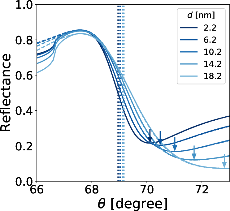
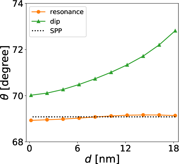
Figure 7 shows the dependences of the reflection spectrum, dip angle, and resonant angle on the radius of the dimple cylinder, ; period of the dimple array, ; and depth of the dimple, . Panels (a) and (d) show the results in the case where the value of is changed from 20 nm to 170 nm while fixing nm and nm. It is observed that as the dimple radius increases, the dip angle (arrows in panel (a)) and resonant angle (dotted lines in panel (a)) shift to the wider-angle side. Note that the change in the dip angle is much larger than that in the resonant angle. Panels (b) and (e) show the results in the case where the value of is changed from 600 nm to 250 nm while fixing nm and 80 nm. It is observed that as the period decreases, the dip angle and resonant angle shift to the wider-angle side. Moreover, the change in the dip angle is larger than that in the resonant angle. Panels (c) and (f) show the results in the case where the value of is changed from 2.2 nm to 18.2 nm while fixing nm and nm. It is observed that as the depth increases, the dip angle and resonant angle shift to the wider-angle side. Moreover, the change in the dip angle is larger than that in the resonant angle.
(a)
(b)
(c)

Figure 8 shows the decay rates, , and , and the direct reflection phase extracted by the TCM method. Panels (a), (b), and (c) show the results for the same condition as that in panels (a), (b), and (c) of Fig. 7, respectively. These results indicate that an increase in , decrease in , or increase in , namely increase in the ratio of the region of dimple in the metal film region, results in an increase in the decay rate and decrease in . However, the increase in the internal decay rate is rather small, and that in the decay rate mainly originates from the increase in the external decay rate . This tendency is similar to that observed when the thickness of a flat metal film is decreased. It can be interpreted that the formation of dimples reduces the effective thickness of the metal film and enhances the radiation from SPP at the NaCl solution side to the substrate side, to increase the external decay rate. The change in can be explained by the decrease in the effective thickness of the metal film, as in a flat metal film.
The trend of is opposite to that in the case of change in the thickness of a flat metal film. This behavior indicates that the diffraction of SPP by the dimple array enhances the internal decay. However, the change in is mainly determined by the material loss (volume of metal region) because the diffraction produced by the periodic array with the period comparable to the wavelength is restricted to a few diffraction orders and the influence on the direct reflection process is weak.
III.5 Random array
For the periodic array discussed in the previous section, the effect of diffusive scattering is weak because the radiative diffraction order is restricted. In this section, we discuss a system with randomly distributed dimples in order to include the effect of diffusive scattering. Figure 9 shows the dependence of (a) the angular spectrum, (b) dip and resonant angles, and (c) decay rates and the direct reflection phase on the depth of dimple for a sample whose extracted values are near the averaged values of randomly produced 100 samples. Here, is set to 80 nm, and is changed from 0.2 nm to 18.2 nm for the same distribution of dimples in the plane. In addition, in this section, the thickness of the aluminum film outside the dimple is assumed to be nm.
Comparing the results for the periodic array in Fig. 7 (c) and (f) and those for the random array in Fig. 9 (a) and (b), it is found that the extension of the width of the dip and the shift of the dip angle due to an increase in are larger in the random array. In addition, Fig. 8 (c) and 9 (c) show that increases with in a random array, contrary to the case of periodic array. These results are similar to those obtained when is increased in a flat metal film. Thus, the introduction of a random dimple array produces a similar effect as that of an increase in metal loss. The diffusive scattering produced by the random array suppresses the direct specular reflection, like absorption.
III.6 Effect of dimple array on parameters
From the above consideration, it is deduced that one of the effects of dimple formation is the reduction in the effective thickness of the aluminum film. This results in an increase in external decay, namely the enhancement of radiation from the resonant mode. The radiation from the resonant mode is limited by the tunneling process within the metal region, which depends exponentially on the product of the decay rate of the evanescent field in the direction, , and the thickness of the metal region. Here, is the wavenumber of SPP at an angular frequency of . Therefore, we define the effective thickness of the metal film as follows:
| (16) |
where the period of array is taken to be 400 nm in the random array case, considering the average density of the dimples.
Figure 10 shows the relation between the value of effective film thickness defined by Eq. (16) and the external decay rate. The black solid line depicts the results for a flat aluminum film with thickness . The light-blue dashed line denotes exponential dependence on , expressed by the left- hand side of Eq. (16), based on the value at nm. All data coincide well, which shows the validity of the estimation of effective thickness using Eq. (16). Thus, we can evaluate from the value of assuming the exponential dependence between them, and use it as an index for corrosion.

In Fig. 11 (a), the values of and extracted from the reflection spectra for various conditions of the periodic array (yellow circles) and random array (green squares) of dimples are plotted on the color map of the spectral shape factor , as in Fig. 6 (c). The black solid line depicts the result of a flat aluminum film with various thicknesses decreasing from the lower right to upper left, where the imaginary part factor is fixed to 1. Using the results shown in Fig. 6 (c), we can deduce the thickness of the aluminum film, , and the imaginary part factor, , for the metal film that provides the values of , , and at the points in Fig. 11 (a). Thus, we obtain a flat metal film model with thickness and imaginary part factor for each dimple array system. This model gives the same shape of the normalized reflection spectrum as the dimple array system. Figure 11 (b) and (c) show and as functions of effective thickness for periodic arrays (red dots), random arrays (green squares), and a flat aluminum film (black solid line). Panel (b) shows that corresponds rather well with , which is consistent with the notion that one of the effects of the dimple array is to reduce the effective thickness of the aluminum film and result in the exponential enhancement of radiative decay. While from panel (c), another effect of the dimple array can be considered to alter (enhance in most cases) the imaginary part of the permittivity of aluminum effectively. This effect seems to be produced by diffusive scattering, which depends on the configuration of the dimples. Indeed, we can see that random arrays provide higher enhancement than the periodic array.
These effects of the dimple array appear in each parameter value, such as the internal decay rate and the direct reflection coefficient , as shown in Fig. 11 (d) and (e). These parameters strongly depend on the structure and distribution of dimples, even though they provide the same effective thickness. Especially, the plots of for the flat films, periodic arrays, and random arrays are distributed separately. These results indicate that a more detailed characterization of the metal surface condition can be achieved by analyzing these parameters systematically, e.g., by using machine learning. However, this will be taken up in the future.
(a)

(b)

(c)

(d)

(e)

IV Conclusions
In this paper, we have shown the possibility of evaluating the surface roughness of a metal film by analyzing the ATR spectrum from the viewpoint of Fano resonance. Using the temporal coupled-mode method, it was found that the geometrical feature of the ATR spectrum is characterized by a single shape factor, which is determined by the following two parameters: direct reflection phase and ratio of decay rates. Based on this information, we have developed a method to extract key parameters, such as internal and external decay rates, from spectral data, and shown that these parameters provide corrosion information such as the effective thickness of the metal film and the distribution of nanosized dimples. These results form the basis for developing a novel method for characterizing the initial stage of pitting corrosion on a metal surface using plasmonic ATR.
Acknowledgments
This study was supported by JSPS KAKENHI Grant Numbers JP18K04980 and JP18K04979.
References
- Liedberg et al. (1983) B. Liedberg, C. Nylander, and I. Lunström, Sensors and Actuators 4, 299 (1983).
- Homola et al. (1999) J. Homola, S. S. Yee, and G. Gauglitz, Sensors and Actuators B: Chemical 54, 3 (1999).
- Homola (2008) J. Homola, Chemical Reviews 108, 462 (2008), pMID: 18229953, https://doi.org/10.1021/cr068107d .
- Kretschmann and Raether (1968) E. Kretschmann and H. Raether, Zeitschrift für Naturforschung A 23, 2135 (1968).
- Kretschmann (1971) E. Kretschmann, Zeitschrift für Physik A Hadrons and nuclei 241, 313 (1971).
- Raether (1988) H. Raether, Surface Plasmons on Smooth and Rough Surfaces and on Gratings (Springer, Berlin, Heidelberg, 1988).
- Vinogradov et al. (2018) A. P. Vinogradov, A. V. Dorofeenko, A. A. Pukhov, and A. A. Lisyansky, Phys. Rev. B 97, 235407 (2018).
- Nesterenko et al. (2018) D. V. Nesterenko, S. Hayashi, and Z. Sekkat, Phys. Rev. B 97, 235437 (2018).
- Fano (1961) U. Fano, Phys. Rev. 124, 1866 (1961).
- Braundmeier and Arakawa (1974) A. Braundmeier and E. Arakawa, Journal of Physics and Chemistry of Solids 35, 517 (1974).
- Hornauer et al. (1974) D. Hornauer, H. Kapitza, and H. Raether, Journal of Physics D: Applied Physics 7, L100 (1974).
- Orlowski et al. (1979) R. Orlowski, P. Urner, and D.-L. Hornauer, Surface Science 82, 69 (1979).
- Sari et al. (1980) S. O. Sari, D. K. Cohen, and K. D. Scherkoske, Phys. Rev. B 21, 2162 (1980).
- Chen et al. (2010) X. Chen, M. Pan, and K. Jiang, Microelectronic Engineering 87, 790 (2010), the 35th International Conference on Micro- and Nano-Engineering (MNE).
- Agarwal et al. (2017) S. Agarwal, Y. Prajapati, and V. Singh, Optics Communications 383, 113 (2017).
- Bussjager and Macleod (1996) R. J. Bussjager and H. A. Macleod, Appl. Opt. 35, 5044 (1996).
- Oliveira et al. (2017) L. C. Oliveira, A. Herbster, C. da Silva Moreira, F. H. Neff, and A. M. N. Lima, IEEE Sensors Journal 17, 6258 (2017).
- Raether (1983) H. Raether, Surface Science 125, 624 (1983).
- Fontana and Pantell (1988) E. Fontana and R. H. Pantell, Phys. Rev. B 37, 3164 (1988).
- Frankel (1998) G. S. Frankel, Journal of The Electrochemical Society 145, 2186 (1998), http://jes.ecsdl.org/content/145/6/2186.full.pdf+html .
- Kaesche (2003) H. Kaesche, Pitting corrosion, in Corrosion of Metals: Physicochemical Principles and Current Problems (Springer Berlin Heidelberg, Berlin, Heidelberg, 2003) pp. 324–388.
- McCafferty (2010) E. McCafferty, Introduction to Corrosion Science (Springer-Verlag New York, 2010).
- Haus (1983) H. A. Haus, Waves and Fields in Optoelectronics (Prentice Hall, Englewood Cliffs, NJ, 1983).
- Fan et al. (2003) S. Fan, W. Suh, and J. D. Joannopoulos, J. Opt. Soc. Am. A 20, 569 (2003).
- Nishida and Kadoya (2018) M. Nishida and Y. Kadoya, in Fano Resonances in Optics and Microwaves, edited by E. Kamenetskii, A. Sadreev, and A. Miroshnichenko (Springer, 2018) Chap. 14, pp. 331–355.
- García-Vidal et al. (2005) F. J. García-Vidal, E. Moreno, J. A. Porto, and L. Martín-Moreno, Phys. Rev. Lett. 95, 103901 (2005).
- Nishida et al. (2015) M. Nishida, N. Hatakenaka, and Y. Kadoya, Phys. Rev. B 91, 235406 (2015).
- Rakić et al. (1998) A. D. Rakić, A. B. Djurišić, J. M. Elazar, and M. L. Majewski, Appl. Opt. 37, 5271 (1998).
- Joannopoulos et al. (2008) J. D. Joannopoulos, S. G. Johnson, J. N. Winn, and R. D. Meade, Photonic Crystals: Molding the Flow of Light, 2nd ed (Princeton University Press, Princeton, NJ, 2008).
- Eriksson (2007) G. Eriksson, in 2007 IEEE International Symposium on Electromagnetic Compatibility (2007) pp. 1–6.
- Weiss (2011) T. Weiss, Advanced numerical and semi-analytical scattering matrix calculations for modern nano-optics, Ph.D. thesis, University of Stuttgart (2011).
Supplemental Material: Evaluation of surface roughness
of metal films using plasmonic Fano resonance in attenuated total reflection
Munehiro Nishida,1,∗ Taisei Matsumoto,1 Hiroya Koga,1
Terukazu Kosako,2 and Yutaka Kadoya1
1Graduate School of Advanced Science of Matter,
Hiroshima University, Higashi-Hiroshima, 739-8530, Japan
2YAZAKI Research and Technology Center, 1500 Mishuku, Susono-city,
Shizuoka, 410-1194, Japan
∗Electronic address: mnishida@hiroshima-u.ac.jp
(Dated: August 11, 2026)
S1 Temporal Coupled Method Considering Absorption in Direct Reflection Process
The temporal coupled mode (TCM) method describes resonant scattering phenomenon by considering the dynamics of cavities attached to ports Haus 1983; Fan et al. 2003; Nishida and Kadoya 2018. The Kretschmann configuration in plasmonic ATR can be modeled by a system such that a cavity with a single resonant mode corresponding to SPP is attached to a single input/output port representing a connection with the incident and reflected waves.
In the case where the cavity couples with the port weakly, the amplitude of the resonant mode with the resonant angular frequency of is described by the following coupled mode equation Haus 1983; Fan et al. 2003; Joannopoulos et al. 2008:
| (S1) | ||||
Here, denotes the internal decay rate due to the loss of the materials composing the cavity and denotes the external decay rate due to the loss by the radiation to the port. Variables and denote the amplitudes incoming and outgoing radiative modes through the port, respectively, where the mode fields are normalized so that equal the powers of the modes. The parameters and denote the magnitude and phase of the direct reflection coefficient, which determines the reflection process in which the incoming wave from the port is reflected directly to the port without resonance excitation. The parameter () denotes the coupling constants between the incoming (outgoing) mode and the cavity mode through the port.
If a continuous wave with angular frequency is incident, the amplitude of the resonant mode is given by
| (S2) |
and the outgoing wave is given by
| (S3) |
If the internal decay, energy absorption in the direct reflection process, and coupling between the cavity and the port are all weak, the parameters , , and are approximately independent of the internal decay rate and the absorption of the direct reflection process. Therefore, the relations among , , and can be derived without considering material loss. Suppose for a while that there is no material loss. In this case, and the direct reflection coefficient can be expressed as . The same discussion as in Fan et al. 2003 applies to this case. From energy-conservation and time-reversal symmetry, we obtain
| (S4) | ||||
| (S5) | ||||
| (S6) |
Therefore,
| (S7) | ||||
| (S8) | ||||
| (S9) | ||||
| (S10) |
Consider the case in which the angular spectra near the resonant angle are obtained using a focused incident light with the angular frequency of , where is the speed of light in vacuum. Assuming that becomes when and the relation between and is linear with the gradient of the group velocity of SPP on the surface of a semi-infinite metal, the -dependence of , namely the dispersion relation of the resonant mode, is expressed as
| (S11) |
The parameters in Eq. (S7), , , , and , are set to the values at , and the reflection coefficient for reads
| (S12) | ||||
| (S13) |
Then, the normalized reflectance is given by the following equation:
| (S14) | ||||
| (S15) |
When , solving the equation , the in-plane wavenumbers and at which is minimum and maximum, respectively, are given as
| (S16) |
and the minimum value and maximum value are given as
| (S17) |
where is the sign of , namely , and
| (S18) |
Thus, total absorption () occurs when
| (S19) |
When , there is no maximum of , and for the minimum,
| (S20) | ||||
| (S21) |
Thus, total absorption () occurs when
| (S22) |
Noting that
| (S23) | ||||
| (S24) |
we obtain
| (S25) |
Then, from Eq. (S17) and Eq. (S25),
| (S26) |
In addition, we obtain
| (S27) | ||||
| (S28) |
S2 Improvement in Spatial Coupled Mode Method
The spatial coupled mode (SCM) method derives a set of coupled equations for waveguide modes of nanoholes perforated in a metal film García-Vidal et al. 2005; de León-Pérez et al. 2008; Nishida et al. 2015; Nishida and Kadoya 2018. The electromagnetic (EM) fields outside the metal film are expressed by a linear combination of plane-wave modes specified by the parallel wave vector and the polarization , where and are the incident parallel wave vector and reciprocal lattice vector of the nanohole array, respectively. The EM fields in the metal film region are expressed by the superposition of the waveguide modes of a nanohole and evanescent plane waves in order to account for the penetration of the EM field into the metal region. Here, we assume that the dielectrics inside the nanohole and outside the metal film are the same with the relative permittivity of .
We use Dirac’s notation to describe the electric field components parallel to the -plane for mode , such that
| (S29) |
Here, the mode index represents the full information of the modes of a nanohole, such as the “HE11 horizontal mode” Roberts 1987. This may also represent the parallel wave vector and the polarization for plane-wave modes. Because the magnetic field components parallel to the -plane are determined by the position-dependent admittance Nishida et al. 2015; Nishida and Kadoya 2018, we use the admittance operator to express them, such that
| (S30) |
For the plane-wave mode in the dielectric, this relation is reduced to
| (S31) | ||||
| (S32) |
where and are the impedance and wavenumber in the vacuum, respectively, and is the -component of the wave vector.
We define the internal product of the two fields as
| (S33) | ||||
| (S34) |
where denotes the complex conjugate. Here, the mode fields are normalized by . Then, the orthogonality condition for the plane-wave modes is expressed as
| (S35) |
However, due to the metal loss, the orthogonality condition for the waveguide modes should be modified as
| (S36) |
based on the Lorentz reciprocity theorem Lorentz 1895; de Hoop 1960; Lalanne et al. 2005.
Consider a metal film with nanohole array located at the region . At the interface between the metal and the dielectric at , the EM fields on the dielectric side, , , and on the metal side, ,, are given by
| (S37) | ||||
| (S38) | ||||
| (S39) | ||||
| (S40) |
Similarly, the EM fields at are given by
| (S41) | ||||
| (S42) | ||||
| (S43) | ||||
| (S44) |
Here, is the propagation constant of the waveguide mode and , with being the dielectric function for the metal.
Using these definitions, the coupled-mode equations can be derived in a similar manner as the original derivation de León-Pérez et al. 2008. Under the condition that the projection of the EM field onto the electric field of the plane wave and that of the magnetic field onto the electric field of the waveguide mode are continuous at the two interfaces at and , we can derive a coupled system of equations for the coefficients of waveguide modes as follows:
| (S47) | ||||
| (S48) | ||||
| (S49) | ||||
| (S50) |
| (S51) |
| (S52) |
where we assume that in the metal film region, the electric field inside the nanohole, , and the magnetic field outside the nanohole, , are orthogonal, and
| (S53) | ||||
| (S54) | ||||
| (S55) |
However, the scattering coefficients and , calculated using Eqs. (S51) and (S52), do not obey the reciprocity relation de Hoop 1960; Potton 2004; Mansuripur and Tsai 2011:
| (S56) | ||||
| (S57) |
Therefore, we define the scattering coefficients that guarantee reciprocity, as
| (S58) | ||||
| (S59) |
Using Eqs. (S58) and (S59), we can calculate the reflection and transmission coefficients between various diffraction orders to form reflection and transmission matrices and . Then, we can define a scattering matrix as
| (S60) |
The full scattering matrix for the multilayer system, including nanohole array layers, can be calculated using recurrence formula Weiss 2011. If the system is divided into two parts whose scattering matrices are given by and , then the total scattering matrix is given by
| (S61) |
where the operation is defined by
| (S62) |
References
- Haus (1983) H. A. Haus, Waves and Fields in Optoelectronics (Prentice Hall, Englewood Cliffs, NJ, 1983).
- Fan et al. (2003) S. Fan, W. Suh, and J. D. Joannopoulos, J. Opt. Soc. Am. A 20, 569 (2003).
- Nishida and Kadoya (2018) M. Nishida and Y. Kadoya, in Fano Resonances in Optics and Microwaves, edited by E. Kamenetskii, A. Sadreev, and A. Miroshnichenko (Springer, 2018) Chap. 14, pp. 331–355.
- Joannopoulos et al. (2008) J. D. Joannopoulos, S. G. Johnson, J. N. Winn, and R. D. Meade, Photonic Crystals: Molding the Flow of Light, 2nd ed (Princeton University Press, Princeton, NJ, 2008).
- García-Vidal et al. (2005) F. J. García-Vidal, E. Moreno, J. A. Porto, and L. Martín-Moreno, Phys. Rev. Lett. 95, 103901 (2005).
- de León-Pérez et al. (2008) F. de León-Pérez, G. Brucoli, F. J. García-Vidal, and L. Martín-Moreno, New J. Phys. 10, 105017 (2008).
- Nishida et al. (2015) M. Nishida, N. Hatakenaka, and Y. Kadoya, Phys. Rev. B 91, 235406 (2015).
- Roberts (1987) A. Roberts, J. Opt. Soc. Am. A 4, 1970 (1987).
- Lorentz (1895) H. A. Lorentz, Versl. Kon. Akad. Wetensch. Amsterdam 4, 176 (1895).
- de Hoop (1960) A. T. de Hoop, Applied Scientific Research, Section B 8, 135 (1960).
- Lalanne et al. (2005) P. Lalanne, J. P. Hugonin, and J. C. Rodier, Phys. Rev. Lett. 95, 263902 (2005).
- Potton (2004) R. J. Potton, Reports on Progress in Physics 67, 717 (2004).
- Mansuripur and Tsai (2011) M. Mansuripur and D. P. Tsai, Optics Communications 284, 707 (2011).
- Weiss (2011) T. Weiss, Advanced numerical and semi-analytical scattering matrix calculations for modern nano-optics, Ph.D. thesis, University of Stuttgart (2011).