Studying polymer diffusiophoresis with Non-Equilibrium Molecular Dynamics
Abstract
We report a numerical study of the diffusiophoresis of short polymers using non-equilibrium molecular dynamics simulations. More precisely, we consider polymer chains in a fluid containing a solute which has a concentration gradient, and examine the variation of the induced diffusiophoretic velocity of the polymer chains as the interaction between the monomer and the solute is varied. We find that there is a non-monotonic relation between the diffusiophoretic mobility and the strength of the monomer-solute interaction. In addition we find a weak dependence of the mobility on the length of the polymer chain, which shows clear difference from the diffusiophoresis of a solid particle. Interestingly, the hydrodynamic flow through the polymer is much less screened than for pressure driven flows.
I Introduction
In a bulk fluid, concentration gradients cannot cause fluid flow. However, a gradient in the chemical potential of the various components in a fluid mixture, can cause a net hydrodynamic flow in the presence of an interface that interacts differently with the different components of the mixture. Such flow induced by chemical potential gradients is usually referred as diffusio-osmosis (see e.g. Anderson and Prieve 1984). The same mechanism that causes diffusio-osmosis can also drive the motion of a colloid, or other mesoscopic moiety, under the influence of chemical potential gradients in embedding fluid. Clearly, if the mesoscopic particle (say a colloid) is very large compared to the characteristic length scale on which adsorption or depletion occurs, it is reasonable to use the Derjaguin approximation Derjaguin et al. 1947; Derjaguin, Churaev, and Muller 1987, i.e. to describe the colloid-fluid interface as locally flat, and thus estimate the speed of diffusiophoresis. However, the Derjaguin approach is likely to fail if the particles that are subject to phoresis are no longer large compared to the range of adsorption/depletion. There is yet another situation where the Derjaguin approach is obviously questionable, namely in the case of particles that do not have a well-defined surface. One particularly important example is the case of diffusiophoresis of polymers: molecules that have a fluctuating shape and an intrinsically fuzzy surface. One manifestation of this fuzziness is the fact that the magnitude of the Kirkwood approximation for the hydrodynamic radius of a long self-avoiding polymer is about 63% of the radius of gyration Clisby and Dünweg 2016: for a smooth sphere, this ratio would be 107% (the Kirkwood expression for is only an approximation: the point is that the averages are different and that hydrodynamic radius is smaller than for a corresponding solid object). This difference implies that the density inhomogeneity of a self-avoiding polymer results in penetration of hydrodynamic flow fields into its outer “fuzzy ” layer. In addition, solutes can diffuse through the polymer. This fuzziness clearly makes it difficult to describe a polymer as a solid sphere surrounded with pure liquid, and hence a Derjaguin approach is questionable. The lack of predictive power of the colloidal approximation was pointed out previously by experiments with -DNA by Palacci et al Palacci et al. 2010; Palacci et al. 2012.
There is another factor that makes diffusiophoresis of polymers unusual: since the driving force for diffusiophoresis comes from an excess (or deficit) of solute in the fluid surrounding the polymer, the stronger a solute is attracted to a polymer, the larger this excess will be. However, a strongly binding solute may result in the collapse of the polymer to a compact globule (scaling exponent 1/3). Hence, unlike in the case of colloids, one cannot assume that the size of polymers subject to diffusiophoresis is independent of the polymer-solute interaction. Furthermore, a solute excess/deficit may not be sufficient for the occurrence of diffusiophoresis: if the solutes are strongly adsorbed onto the polymer, they become effectively immobile relative to the polymer, in which case the excess/deficit do not contribute to diffusiophoresis.
In this paper, we report systematic molecular dynamic simulations of diffusiophoretic transport of short polymers. Specifically, we apply non-equilibrium molecular dynamic simulations using a microscopic force acting on each species, and examine the effect of interaction parameters between the monomer and the solute on the induced diffusiophoretic velocity of the polymer. Our simulations indeed reveal a non-monotonic dependence of the phoretic mobility on , the interaction strength between the polymer and solute. We have investigated the influence of the size of the polymer on its diffusiophoretic mobility. We find a weak polymer-size dependence of the mobility. We compare these findings with the corresponding theoretical predictions for a colloidal particle.
II Thermodynamics forces and their microscopic representation
Conceptually the most straightforward way of simulating diffusiophoresis would be to carry out a Non-Equilibrium Molecular Dynamics (NEMD) with an imposed concentration gradient, following a procedure similar to Heffelfinger and Van Swol Heffelfinger and Swol 1994 and Thompson and Heffelfinger Thompson and Heffelfinger 1999. Nonetheless, there are several drawbacks associated with this approach for modeling diffusiophoresis, the most significant being that periodic boundary conditions are incompatible with the existence of constant concentration gradients as advection deforms the concentration profiles (see Supplementary Material). However, in analogy with simulations of systems in homogeneous electrical fields, we can replace the gradient of a chemical potential by an equivalent force per particle that can be kept constant, and therefore compatible with periodic boundary conditionsYoshida, Marbach, and Bocquet 2017; Liu, Ganti, and Frenkel 2018. This field-driven non-equilibrium approach has been often applied in other contexts Evans and Morriss 2008. The idea is to impose a mechanical constraint (i.e an external field) that mimics the effect of the force Ciccotti, Jacucci, and McDonald 1979. To see how this approach works in the systems that we study, we first consider diffusio-osmosis in a binary mixture of solvent () and solute () particles, which are subjected to a gradient of chemical potential of one of the species (e.g. ), and a gradient in the pressure (in bulk fluids in the absence of external body forces, the pressure gradient will typically vanish). We assume that the system is at constant temperature. Ajdari and Bocquet Ajdari and Bocquet 2006 derived an expression for the transport matrix that relates the fluxes,viz. the total volume flow and the excess solute flux , with the gradient of pressure and the gradient of the chemical potential of one of the species; where is the solute concentration in the bulk . There are only two independent thermodynamic driving forces as, at constant temperature, only two of the three quantities , the solute and the solvent are independent. In fact, it is convenient to define a slightly modified chemical potential gradient by , in which is the ratio between the solute (s) and solvent (f) concentrations in the bulk. With this definition, the linear transport equations can be written as
| (1) |
where ’s are the Onsager transport coefficients connecting the different fluxes with the thermodynamic driving forces. In what follows, it is convenient to replace the gradient of the chemical potential on species by an equivalent external force , such that . This approach to replace the chemical potential gradient by an equal (and opposite) “color” force was previously used in the context of diffusion and transport in microporous materials by Maginn et al. Maginn, Bell, and Theodorou 1993; Arya, Chang, and Maginn 2001. In the context of diffusio-osmosis, Liu et al. Liu, Ganti, and Frenkel 2018 showed that simulations using color forces yield the same results as those obtained with explicit gradients of concentration. Furthermore, Yoshida et al. Yoshida, Marbach, and Bocquet 2017 used the Green-Kubo formalism Hansen and McDonald 2006 to show that Onsager’s reciprocity is also fulfilled. Ganti et al. have applied and validated a similar approach in the context thermo-osmosis Ganti, Liu, and Frenkel 2017a; Ganti, Liu, and Frenkel 2017b.
Having considered the case of a binary solvent-solute mixture, we now add a third component, namely the polymer, to the system. Again, not all chemical potential gradients are independent, as it follows from the Gibbs-Duhem equation:
| (2) |
In what follows, we assume there are no global pressure and thermal gradients in the system. As a consequence, we can write:
| (3) |
where ,, denote the equivalent forces on the polymer, solute and solvents mimicking the corresponding chemical potential gradients. , refer to the total number of solutes and solvents in the system as a whole. This equation simply expresses the fact that there can be no net external force on the fluid: if there were, the system would accelerate without bound, as there are no walls or other momentum sinks in the system. In simulations, it is convenient to work with a force per monomer, rather than a force on the center-of-mass of the polymer: , where denotes the number of beads in the polymer. Equation (3) establishes a connection between all chemical potential gradients (or the corresponding microscopic forces), which must be balanced throughout the system as phoretic flow cannot cause bulk flow.
We will now compute the rate of polymer diffusiophoresis using Eq. (3) as our starting point.
III Molecular Dynamics (MD) simulations
We performed non-equilibrium Molecular Dynamics (NEMD) simulations using LAMMPS Plimpton 1995. In most simulations, particles interact via a 12-6 Lennard-Jones potential (LJ) shifted and truncated at , such that
| (4) |
The indices and denote the particle types in our simulations: solutes (), solvents () and monomers (). To keep the model as simple as possible, we assume that in the bulk the solute and solvent behave as an ideal mixture. We therefore choose the same Lennard-Jones interaction for the particle pairs , , with and . We use these same parameters also for the monomer-solvent interaction . However, the monomer-solute interaction strength was varied to control the degree of solute adsorption or depletion around the polymer. Yet, we kept equal to . For the monomer-monomer interaction, we use a purely repulsive Weeks-Chandler-Andersen potential Weeks, Chandler, and Andersen 1971, i.e. a Lennard-Jones potential truncated and shifted at the minimum of the LJ potential, . For all other interactions, . Finally, neighboring monomers are connected by a finite extensible, nonlinear elastic (FENE) anharmonic potential , Bishop, Kalos, and Frisch 1979; Dünweg and Kremer 1993
| (5) |
with and . In what follows, we use the mass of all the particles (, and ) as our unit of mass and we set our unit of energy equal to , whilst our unit of length is equal to , all other units are subsequently expressed in term of these basic units. As a result, forces are expressed in units , and our unit of time is .
III.1 Equilibration
We studied the diffusiophoresis of a single polymer chain composed of 30 monomers, , suspended in an equimolar ideal mixture of solute and solvent molecules.
The initial simulation box dimensions were , , and the number of fluid particles was 8748.
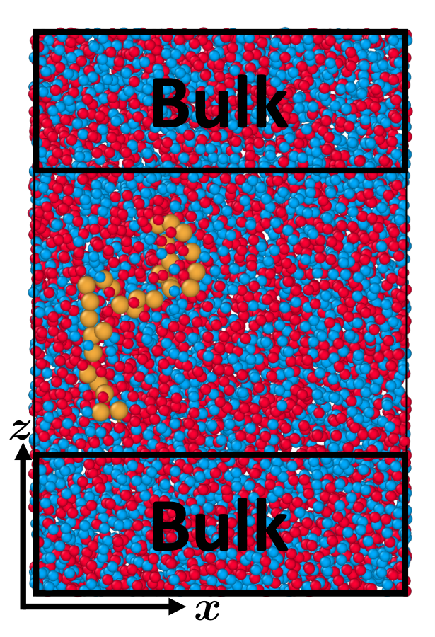
After equilibration, chemical potential gradients were applied along the -axis. We distinguished two types of domains in the simulation box: one periodically repeated domain with width in the -direction centered around the polymer’s center of mass in the -coordinate. The remainder of the system ( a domain with width ), contains only bulk fluid (see Fig 1 – note that because this figure is centered around the polymer, one half of the bulk domain is shown above and one half below the polymer domain). We verified that the composition of the mixture in this bulk domain is not influenced by the presence of the polymer in the other domain (See Supplementary material). The system is periodically repeated on each direction.
Our aim was to carry out simulations under conditions where the composition of the bulk fluid was kept fixed, even as we varied the monomer-solute interaction. Moreover, we prepared all systems at the same hydrostatic pressure. Therefore, we performed NPT simulations using a Nosé-Hoover thermostat/barostat Hoover 1985. The equations of motion were integrated using a velocity-Verlet algorithm with time step . After the relaxation of the initial configuration, the box was allowed to fluctuate in the direction, fixing and for steps.
During the NPT equilibration, fixing the bulk concentration of the liquid requires a careful protocol, in particular in cases where the solute binds strongly to the polymer. In our simulations, we accelerated the equilibration of the solute adsorption on the polymer by attempting to swap solvent and solute molecules times for every MD step throughout the simulation box. Simultaneously, we swapped solutes and solvents in the bulk, to ensure that adsorption on the polymer does not deplete the solute concentration in the bulk. To this end, we swapped solutes and solvents in the bulk every 200 steps such that the bulk solute concentration remained fixed at . Note that these swaps were only carried out during equilibration.
III.2 Field-driven simulation
Having prepared a system of polymer in a fluid mixture with a pre-determined pressure and bulk composition, we now consider the effect of chemical potential gradients on the phoretic motion of the polymer in NVT simulations. As discussed above, we represent the chemical potential gradients by equivalent external forces that are compatible with the periodic boundary conditions. Importantly, the forces are chosen such that a) there is no net force on the system as a whole and b) there is no net force on the bulk solution away from the polymer. These two conditions imply that there is only one independent force that can be defined in the system. In the present case, we chose to fix the force on the solutes , which was varied between and for different runs. During all the field-driven simulations, we employed a dynamical definition of the bulk and polymer domains such that the -coordinate of the center of mass of the polymer is always in the middle of the polymer domain. This procedure ensures that the “bulk” region remains unperturbed by the polymer. Having specified the force on the solute, the force on the solvent particles follows from mechanical equilibrium in the bulk in Eq. (3) (see Fig. 1):
| (6) |
where , denote the number of solutes and solvent in the bulk region. Once the forces in the bulk have been specified, the phoretic force on the polymer is obtained by imposing force balance on the system as a whole (Eq. (3)).
Due to the finite size of the bulk domain there are inevitably fluctuations in the composition of this domain. These fluctuations would lead to unphysical velocity fluctuations in the bulk (unphysical because in the thermodynamic limit this effect goes away). These velocity fluctuations would contribute to the noise in the observed phoretic flow velocity. To suppress this effect, we could either adjust the composition in the bulk domain at every time step, or adjust the forces on solute and solvent ( and ) such that the external force on the bulk domain is always rigorously equal to zero. We opted for the latter approach, because particle swaps would affect the stability of the MD simulations.
IV Results and discussion
IV.1 Phoretic velocity
In Fig 2 the polymer velocities in the direction of the gradient are plotted for three different pair of LJ parameters. When there is adsorption of solutes around the polymer (, the polymer follows the gradient, migrating towards regions where the solute concentration is higher. Conversely, when there is depletion ( the polymer will move in the opposite direction. As a null check, we also performed simulations for the case where the . In that case, there should be no phoresis, as is indeed found in the data shown in Fig. 2. The inversion of the velocity depending on the sign of the monomer-solute interaction is expected on the basis of irreversible thermodynamics Anderson and Prieve 1984 and has previously been observed in simulations of for nano-dimers, using hybrid molecular dynamics-multiparticle collision (MD-MPC) dynamics Rückner and Kapral 2007; Tao and Kapral 2008.
The figure also shows that our simulations appear to be in the linear regime, as the magnitude of the phoretic velocity increases linearly with the strength of the applied field.
IV.2 Mobility dependence on the interaction
The mobility of a polymer moving under the influence of a gradient in the solute chemical potential is defined through:
| (7) |
We can compute as a function of the polymer-solute interaction strength from the slope of the vs. plots, such as the ones shown in Fig 2. This procedure allows us to obtain as a function of the monomer-solute interaction strength . We stress that, whilst we determine by varying , we keep the bulk composition of the mixture fixed (as well as the temperature and the pressure). The resulting relation between and is shown in Fig 3. As expected, is linear in when is close to one. However, as the monomer-solute interaction gets stronger, saturates, and subsequently decays with increasing .
The observed decrease of for large values of suggests that when solute particles bind strongly to the polymer, they become effectively immobilised and hence cannot contribute to the diffusio-osmotic flow through and around the polymer. This argument would suggest that the diffusiophoretic velocity should vanish as becomes much larger than the thermal energy. However, that does not seem to be the case: rather seems to level off at a small but finite value. This suggests that not all fluid particles involved in the phoretic transport are tightly bound to the polymer. One obvious explanation could be that the LJ potential that we use is sufficiently long-ranged to interact with solute particles that are in the second-neighbour shell around the monomeric units of the polymer. To test whether this is the case, we repeated the simulations with a shorter-ranged short-ranged Lennard-Jones-like potential (SRLJ)Wang et al. 2019 that has a smaller cut-off distance ( ) where the potential and its first derivative vanish continuously. In the insert of Fig. 3 this narrower potential is shown compared with the standard truncated and shifted LJ potential with , and . In our simulations we only used the SRLJ potential for the monomer-solute interactions. For all other interactions we still use the standard LJ potential.
Figure 3 shows a comparison of the results obtained with the LJ and the SRLJ potentials. Interestingly, even with the short-ranged monomer-solute interaction for which next-nearest neighbour interactions are excluded, still does not decay to zero at large . This suggests that the phoretic force is not just probing the excess of solute particles that are directly interacting with the polymer, but also the density modulation of solutes (and solvent) that is due to the longer-ranged structuring of the mixture around the polymer coil. In Fig. 4, we show an extreme case () where the polymer has collapsed and particles within a hydrodynamic radius from the center of mass do not contribute to phoresis as they are tightly bound. In contrast, particles in the structured liquid layer further away from the center of the polymer () are mobile and can therefore contribute to the diffusio-osmotic flow.
IV.3 Scaling of the phoretic mobility with the length of the polymer
For colloidal particles with a radius much larger than the range of the colloid solute interaction, the diffusiophoretic mobility is independent of the colloidal radius Anderson, Lowell, and Prieve 1982. As the diffusion of a polymer in a fluid is often described as that of a colloid with an equivalent “hydrodynamic radius” , one might be inclined to assume that the diffusiophoretic mobility of a sufficiently large polymer might also be size independent. To our knowledge, this size dependence has not been tested in simulations. However, experiments by Rauch and Köhler Rauch and Köhler 2005 showed that thermophoretic mobility of polymers varies with the molecular weight for short polymers (fewer than 10 monomers), but very little for longer polymers (10-100 monomers).
For colloids, Anderson Anderson, Lowell, and Prieve 1982 derived an expression for the diffusiophoretic mobility of colloids in the case where the interfacial layer thickness is smaller, but not much smaller than the radius of the colloid. Introducing the small parameter , Anderson derived the following asymptotic expression for the diffusiophoretic velocity of a colloidal particle:
| (8) |
In this approximation, the first term corresponds to the Derjaguin limit :
| (9) |
where is the magnitude of the concentration gradient, , is the shear viscosity and is the potential of mean force experienced by solutes at a distance from the surface of the colloid. , , are proportional to moments of the excess solute distribution ,
| (10) |
| (11) |
| (12) |
The corrections terms in Eq. (8) account for the effect of the curvature of the particle. All the above equations apply to the case where there is no hydrodynamic slip on the surface of the colloid. However, if solute particles are strongly adsorbed to the colloid, they become immobile and the result is simply that the surface of no slip, and hence the effective colloidal radius, increases. Eq. (8) was derived assuming no-slip boundary conditions to solve the Navier-Stokes equation. However, Ajdari and Bocquet Ajdari and Bocquet 2006 showed that a correction due to the hydrodynamic slip captures the transport enhancement at interfaces. Including the amplification factor due the surface slip, for moderate adsorption or depletion of solutes, the corrected diffusiophoretic velocity reduces to:
| (13) |
where is the hydrodynamic slip length.
To study the dependence of the phoretic motion of a polymer on the number of monomers of the chain , simulations were performed for a range of from to . As our polymers are fully flexible (but self-avoiding) a chain of 60 beads corresponds to a medium-sized polymer. The simulation box was scaled accordingly with the Flory exponent for a polymer in a good solvent thus ensuring that the chain could not overlap with its periodic images. All the NEMD simulations were carried out for time steps.
In Fig. 5, the simulation results are shown together with theoretical predictions replacing the polymer by an equivalent hard sphere with a radius , with the hydrodynamic radius given by Stokes-Einstein relation (Comparison with the Kirkwood approximation for Kirkwood 1954 are shown in SI ),
| (14) |
where denotes the viscosity of the solution in the bulk, which was computed independently, using the Green-Kubo expression relating to the stress auto-correlation function, in an equilibrium simulation of the bulk fluid (see, e.g. Hansen and McDonald 2006). The diffusion coefficient was also computed from equilibrium simulations Frenkel and Smit 2002 taking into account the different interactions . Fig. 5 shows that the diffusiophoretic mobility of the polymer increases with . The large quantitative differences between the simulations and the theoretical approximations for a colloid with the same hydrodynamic radius are to be expected: First of all, the assumption that the polymer coil behaves as a hard sphere with is rather drastic. To be more precise, this approximation (that was also used by Kirkwood Kirkwood 1954) assumes that the liquid molecules within the coil region move together, such that the whole assembly moves as a rigid sphere (see e.g. Strobl 2007). This might be a good approximation for the diffusion of long polymer coils, but in the case of phoresis, it is unrealistic to assume that no solute/solvent can be transported through the polymer at distances less than . The second (but related) questionable approximation is that defines the surface of the equivalent colloid in the integrals in Eqs. (10)-(12). As a consequence, the contribution of any excess solute at a distance less than from the polymer center is ignored. As is clear from Fig. 4 this assumption is incorrect and is likely to underestimate the real diffusiophoretic flow, in view of the fact that Fig. 6(b) shows that there can be considerable solute advection for .
Our simulations suggest that better theoretical models for polymer diffusiophoresis are needed. In Fig. 6 we show the velocity field for a polymer with for two cases: when it is subjected to a body force i.e pressure gradient 6(a) and under the influence of diffusiophoresis 6(b). As is obvious from the figure, in both cases there is fluid motion within the polymer at distances less than from its center of mass. However, there is an important difference between the flows inside the polymer for the pressure-driven and phoretically driven flows: strong hydrodynamic screening is found in the case of a pressure gradient while for diffusiophoresis, screening seems to be effectively absent. Notice that the density profile is somewhat asymmetric due to the advection produced by the pressure-driven flow.
Shin et al. reported evidence for a similar absence of hydrodynamic screening in a dense plug of colloidal particles moving under the influence of diffusiophoresis Shin et al. 2017. Shin et al. argued that the difference in screening in the case of phoretic flow, as opposed to flow due to body forces or pressure gradients, could be attributed to the difference in the range of the hydrodynamic flow fields in these two cases (() for body-forces and pressure driven flow, () of phoretically induced flows Anderson 1989.
V Conclusions
We have performed molecular dynamics simulation on the diffusiophoresis of polymers in a fluid mixture under the influence of a concentration gradient of solutes. In our non-equilibrium molecular dynamics simulation, we mimicked the effect of an explicit concentration gradient in the system by imposing equivalent microscopic forces on the solute, solvent and monomers. This approach allows us to use periodic boundary conditions and facilitates a systematic investigation of diffusiophoresis. Our results reveal a non-monotonic relation between the diffusiophoretic mobility and the interaction strength between the polymer and the solute. The findings imply that, in the strong interaction regime, the phoretic mobility decreases with increasing monomer-solute interaction strength. This result can be understood by noting that solutes that are strongly bound to the polymer cannot contribute to diffusiophoresis. Furthermore, we have demonstrated that the diffusiophoretic mobility of a (short) polymer cannot be explained in terms of a model that assumes that polymers behave like colloids with the same hydrodynamic radius. Finally, we found effectively no screening of hydrodynamic flow inside a polymer moving due to diffusiophoresis, as opposed to what is observed in the case of a polymer that is moved through a fluid by an external force.
VI Supplementary Material
In the supplementary material we show the concentration distribution of solvent, solute, and solution as a function of radial coordinate from the center of mass of the polymer for . We discuss simulations of a single, fixed colloid in a concentration gradient, and finally we show the diffusiophoretic mobilities of the polymer vs the number of monomers in the polymer and compare with theoretical predictions based on the Kirkwood approximation for the hydrodynamic radius.
VII Acknowledgements
This work was supported by the European Union Grant No. 674979 [NANOTRANS]. DF and LB acknowledge support from the Horizon 2020 program through 766972-FET-OPEN-NANOPHLOW. We would like to thank Richard P. Sear, Raman Ganti, Stephen Cox and Patrick Warren for the illuminating discussions.
VIII Data Availability
The data that support the findings of this study are available from the corresponding author upon reasonable request.
References
- Anderson and Prieve (1984) J. L. Anderson and D. C. Prieve, Separation and Purification Methods 13, 67 (1984).
- Derjaguin et al. (1947) B. V. Derjaguin, G. P. Sidorenkov, E. A. Zubashchenkov, and E. V. Kiseleva, Kolloidn. zh 9, 335 (1947).
- Derjaguin, Churaev, and Muller (1987) B. Derjaguin, N. Churaev, and V. Muller, Surface Forces (Springer Science+Business Media, LLC, 1987) p. 398.
- Clisby and Dünweg (2016) N. Clisby and B. Dünweg, Physical Review E 94, 052102 (2016).
- Palacci et al. (2010) J. Palacci, B. Abécassis, C. Cottin-Bizonne, C. Ybert, and L. Bocquet, Physical Review Letters 104, 138302 (2010).
- Palacci et al. (2012) J. Palacci, C. Cottin-Bizonne, C. Ybert, and L. Bocquet, Soft Matter 8, 980 (2012).
- Heffelfinger and Swol (1994) G. S. G. Heffelfinger and F. v. Swol, Journal of Chemical Physics 100, 7548–7552 (1994).
- Thompson and Heffelfinger (1999) A. P. Thompson and G. S. Heffelfinger, The Journal of Chemical Physics 110, 10693 (1999).
- Yoshida, Marbach, and Bocquet (2017) H. Yoshida, S. Marbach, and L. Bocquet, Journal of Chemical Physics 146, 194702 (2017).
- Liu, Ganti, and Frenkel (2018) Y. Liu, R. Ganti, and D. Frenkel, Journal of Physics Condensed Matter 30, 205002 (2018).
- Evans and Morriss (2008) D. J. Evans and G. Morriss, Statistical Mechanics of Nonequilibrium Liquids, 2nd ed. (Cambridge University Press, 2008).
- Ciccotti, Jacucci, and McDonald (1979) G. Ciccotti, G. Jacucci, and I. R. McDonald, Journal of Statistical Physics 21, 1 (1979).
- Ajdari and Bocquet (2006) A. Ajdari and L. Bocquet, Physical Review Letters 96, 186102 (2006).
- Maginn, Bell, and Theodorou (1993) E. J. Maginn, A. T. Bell, and D. N. Theodorou, The Journal of Physical Chemistry 97, 4173 (1993).
- Arya, Chang, and Maginn (2001) G. Arya, H. C. Chang, and E. J. Maginn, Journal of Chemical Physics 115, 8112 (2001).
- Hansen and McDonald (2006) J. P. Hansen and I. R. McDonald, Theory of simple liquids, 3rd ed. (Academic Press, 2006).
- Ganti, Liu, and Frenkel (2017a) R. Ganti, Y. Liu, and D. Frenkel, Physical Review Letters 119, 038002 (2017a).
- Ganti, Liu, and Frenkel (2017b) R. Ganti, Y. Liu, and D. Frenkel, Physical Review Letters 121, 068002 (2017b).
- Plimpton (1995) S. Plimpton, Journal of Computational Physics 117, 1 (1995).
- Weeks, Chandler, and Andersen (1971) J. D. Weeks, D. Chandler, and H. C. Andersen, Journal of Chemical Physics 54, 5237 (1971).
- Bishop, Kalos, and Frisch (1979) M. Bishop, M. H. Kalos, and H. L. Frisch, Journal of Chemical Physics 70, 1299 (1979).
- Dünweg and Kremer (1993) B. Dünweg and K. Kremer, The Journal of Chemical Physics 99, 6983 (1993).
- Hoover (1985) W. G. Hoover, Physical Review A 31, 1695 (1985).
- Rückner and Kapral (2007) G. Rückner and R. Kapral, Physical Review Letters 98, 13 (2007).
- Tao and Kapral (2008) Y. G. Tao and R. Kapral, Journal of Chemical Physics 128 (2008), 10.1063/1.2908078.
- Wang et al. (2019) X. Wang, S. Ramírez-Hinestrosa, J. Dobnikar, and D. Frenkel, Physical Chemistry Chemical Physics (2019).
- Anderson, Lowell, and Prieve (1982) J. L. Anderson, M. E. Lowell, and D. C. Prieve, Journal of Fluid Mechanics 117, 107 (1982).
- Rauch and Köhler (2005) J. Rauch and W. Köhler, Macromolecules 38, 3571 (2005).
- Kirkwood (1954) J. G. Kirkwood, Journal of Polymer Science 12, 1 (1954).
- Frenkel and Smit (2002) D. Frenkel and B. Smit, Academic, New York, 2nd ed. (Academic Press, 2002).
- Strobl (2007) G. Strobl, The Physics of Polymers: Concepts for Understanding their Structure and Behavior, 3rd ed. (Springer-Verlag, 2007).
- Shin et al. (2017) S. Shin, J. T. Ault, P. B. Warren, and H. A. Stone, Physical Review X 7, 041038 (2017).
- Anderson (1989) J. L. Anderson, Annual Review of Fluid Mechanics 21, 61 (1989).