Bayesian parameter estimation using conditional variational autoencoders for gravitational-wave astronomyPreprint: APS/123-QED
GW (GW) detection is now commonplace Abbott et al. 2019; Abbott et al. 2021a; Abbott et al. 2017 and as the sensitivity of the global network of GW detectors improves, we will observe on the order of 100s of transient GW events per year Abbott et al. 2018. The current methods used to estimate their source parameters employ optimally sensitive Searle et al. 2009 but computationally costly Bayesian inference approaches Veitch et al. 2014 where typical analyses have taken between 6 hours and 6 days gra. For BNS (BNS) and NSBH (NSBH) systems prompt counterpart EM (EM) signatures are expected on timescales of 1 second – 1 minute and the current fastest method for alerting EM follow-up observers Singer and Price 2016, can provide estimates in on the order of 1 minute, on a limited range of key source parameters. Here we show that a CVAE (CVAE) Tonolini et al. 2020; Pagnoni et al. 2018 pre-trained on BBH (BBH) signals can return Bayesian posterior probability estimates. The training procedure need only be performed once for a given prior parameter space and the resulting trained machine can then generate samples describing the posterior distribution orders of magnitude faster than existing techniques.
The problem of detecting GW has largely been solved through the use of template based matched-filtering, a process recently replicated using machine learning techniques George and Huerta 2018; Gabbard et al. 2018; Gebhard et al. 2017. Once a GW has been identified through this process, Bayesian inference, known to be the optimal approach Searle et al. 2009, is used to extract information about the source parameters of the detected GW signal.
In the standard Bayesian GW inference approach, we assume a signal and noise model and both may have unknown parameters that we are either interested in inferring or prefer to marginalise away. Each parameter is given a prior astrophysically motivated probability distribution and in the GW case, we typically assume a Gaussian additive noise model (in reality, the data is not truly Gaussian). Given a noisy GW waveform, we would like to find an optimal procedure for inferring some set of the unknown GW parameters. Such a procedure should be able to give us an accurate estimate of the parameters of our observed signal, whilst accounting for the uncertainty arising from the noise in the data.
According to Bayes’ Theorem, a posterior probability distribution on a set of parameters, conditional on the measured data, can be represented as
| (1) |
where are the parameters, is the observed data, is the posterior, is the likelihood, and is the prior on the parameters. The constant of proportionality, which we omit here, is , the probability of our data, known as the Bayesian evidence or the marginal likelihood. We typically ignore since it is a constant and for parameter estimation purposes we are only interested in the shape of the posterior.
Due to the size of the parameter space typically encountered in GW parameter estimation and the volume of data analysed, we must stochastically sample the parameter space in order to estimate the posterior. Sampling is done using a variety of techniques including Nested Sampling Skilling 2006; Veitch et al. 2017; Speagle 2019 and Markov chain Monte Carlo methods Foreman-Mackey et al. 2013; Vousden et al. 2015. The primary software tools used by the LIGO (LIGO) parameter estimation analysis are LALInference and Bilby Veitch et al. 2014; Ashton et al. 2018, which offer multiple sampling methods.
Machine learning has featured prominently in many areas of GW research over the last few years. These techniques have shown to be particularly promising in signal detection George and Huerta 2018; Gabbard et al. 2018; Gebhard et al. 2017, glitch classification Zevin et al. 2017, earthquake prediction Coughlin et al. 2017, and to augment existing Bayesian sampling methods Graff et al. 2012. We also highlight recent developments in GW parameter estimation (independent to this work) where one- and two-dimensional marginalised Bayesian posteriors are produced rapidly using neural networks Chua and Vallisneri 2019, and where normalised flows in conjunction with CVAE can reproduce Bayesian posteriors for a single GW detector case Green et al. 2020; Green and Gair 2021. These methods, including the one presented in this paper, are known as “likelihood-free” approaches in which there is no requirement for explicit likelihood evaluation Cranmer et al. 2020, only the need to sample from the likelihood. Nor is it the case that pre-computed posterior distributions are required in the training procedure.
Recently, a type of neural network known as CVAE was shown to perform exceptionally well when applied towards computational imaging inference Tonolini et al. 2020; Sohn et al. 2015, text to image inference Yan et al. 2015, high-resolution synthetic image generation Nguyen et al. 2016 and the fitting of incomplete heterogeneous data Nazabal et al. 2018. CVAE, as part of the variational family of inference techniques are ideally suited to the problem of function approximation and have the potential to be significantly faster than existing approaches. It is therefore this type of machine learning network that we apply in the GW case to accurately approximate the Bayesian posterior , where represents the physical parameters that govern the GW signal, and are the quantities we are interested in inferring. The data represents the noisy measurement containing the GW signal and obtained from a network of GW detectors.
The construction of a CVAE begins with the definition of a quantity to be minimised (referred to as a cost function). In our case we use the cross entropy, defined as
| (2) |
between the true posterior and , the parametric distribution that we will use neural networks to model and which we aim to be equal to the true posterior. The parametric model is constructed from a combination of 2 (encoder and decoder) neural networks and where
| (3) |
In this case the subscripts represent sets of trainable neural network parameters and the variable represents locations within a latent space. This latter object is typically a lower dimensional space within which an encoder can represent the input data, and via marginalisation allows the construction of a rich family of possible probability densities.
Starting from Eq. 2 it is possible to derive a computable bound for the cross-entropy that is reliant on the and networks and a third “recognition” encoder network governed by the trainable parameter-set . The details of the derivation are described in the methods section and in Tonolini et al. 2020 but equate to an optimisation of the ELBO (ELBO). The final form of the cross-entropy cost function is given by the bound
| (4) |
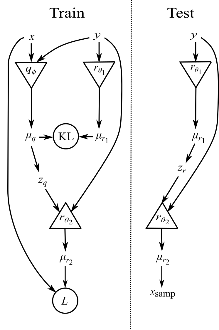
which is also represented graphically in Fig. 1. The cost function is composed of 2 terms, the “reconstruction” cost which is a measure of how well the decoder network predicts the true signal parameters , and the KL (KL)-divergence cost that measures the similarity between the distributions modelled by the and encoder networks. In practice, for each iteration of the training procedure, the integrations over and are approximated by a sum over a batch of draws from the user defined prior , the known likelihood , and the recognition function . Details of the training procedure are given in the methods section.
The implementation of the CVAE that we employ in this letter has a number of specific features that were included in order to tailor the analysis to GW signals. The details of these enhancements are described in the Methods section but in summary, the primary modifications are as follows, 1) Physically appropriate output decoder distributions are used for each output parameter: von Mises-Fisher distribution on the sky location parameters, von Mises distributions on all parameters with cyclic prior bounds, and truncated Gaussians for parameters with defined prior bounds. 2) Each of the functions , and are modelled using deep convolutional neural networks with multi-detector time-series represented as independent input channels. 3) The encoder models an component Gaussian mixture model within the dimensional latent space in order to capture the corresponding typical multi-modal nature of GW posterior distributions. 4.) All cyclic parameters are represented as points in an abstract 2D plane.
We present results on multi-detector GW test BBH waveforms in simulated advanced detector noise ali from the LIGO Hanford, Livingston and Virgo detectors. We compare between variants of the existing Bayesian approaches and our CVAE implementation which we call VItamin 11 1 https://github.com/hagabbar/VItamin.git. Posteriors produced by the Bilby inference library Ashton et al. 2018 are used as a benchmark in order to assess the efficiency and quality of our machine learning approach with the existing methods for posterior sampling.
For the benchmark analysis we assume that 14 parameters are unknown: the component masses , the luminosity distance , the sky position , the binary inclination , the GW polarisation angle , the time of coalescence , and the spin parameters . We do not include phase in our results because we apply phase marginalisation to all Bayesian samplers since this improves overall stability and runtime Ashton et al. 2018.For each parameter we use a uniform prior with the exception of the declination, inclination, and tilt angle parameters for which we use priors uniform in , , , and respectively. The prior on the component masses are conditional, such that . The corresponding prior ranges are defined in Table 2 and result in a SNR (SNR) distribution that has a median value of and ranging between 0 and 75. We use a sampling frequency of Hz, a time-series duration of 1 second, and the waveform model used is IMRPhenomPv2 Khan et al. 2018 with a minimum cutoff frequency of Hz. For each input test waveform we run the benchmark analysis using multiple sampling algorithms available within Bilby. For each run and sampler we extract on the order of 8000 samples from the posterior on the 14 physical parameters.
The VItamin training process uses as input whitened waveforms corresponding to parameters drawn from the same priors as assumed for the benchmark analysis. The waveforms are also of identical duration, sampling frequency, and use the same waveform model as in the benchmark analysis. The signals are whitened22 2 The whitening is used primarily to scale the input to a magnitude range more suitable to neural networks. The true PSD (PSD) does not have to be used for whitening, but training data and test data must be contain signals that share the same PSD. using the same advanced detector PSD ali as assumed in the benchmark analysis. When each whitened waveform is placed within a training batch it is given a unique detector Gaussian noise realisation (after signal whitening this is simply zero mean, unit variance Gaussian noise). The VItamin posterior results are produced by passing each of our whitened noisy testing set of GW waveforms as input into the testing path of the pre-trained CVAE (Fig. 1). For each input waveform we sample until we have generated posterior samples on 15 physical parameters, collectively denoted here as . Comparison results between VItamin and Bayesian samplers do not use since it is marginalised out in the Bayesian sampler inference process.

We can immediately illustrate the accuracy of our machine learning predictions by directly plotting 2 and one-dimensional marginalised posteriors generated using the output samples from our VItamin and Bilby approaches superimposed on each other. We show this for one example test dataset in Fig. 2 where strong agreement between the Bilby sampler Dynesty in blue, and the CVAE (red) is clear. It is also evident that whilst we refer to the Bilby sampler results as benchmark cases, different existing samplers do not perfectly agree with each other (i.e. ptemcee in green) despite using expert recommended sampler settings shown in Tab. 4. For each of our 250 test cases we see reasonable levels of agreement between pairs of benchmark samplers and between any benchmark sampler and our CVAE results.
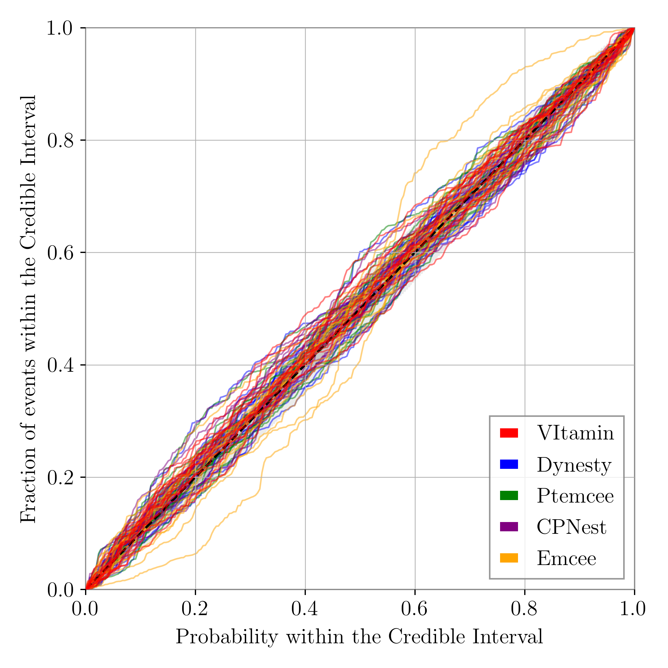
Figures 4 and 5 (see the Methods section) show the results of 2 statistical tests (the PP (PP) plot test and JS (JS)-divergence tests) performed on the entire test dataset and between all samplers (Dynesty, ptemcee, CPNest, emcee, and VItamin). In both tests the quality of the VItamin results are reasonably consistent with the benchmark samplers. The PP plot results specifically indicate that the Bayesian one-dimensional marginalised posteriors from each approach are self-consistent from a frequentist perspective (e.g., the true values lie within the confidence interval for of the test cases). The second test computes the distribution of JS-divergences between posteriors conditioned on the same test data from the “gold standard” benchmark sampler Dynesty and every other benchmark sampler (including VItamin). This measure of “ distribution similarity” shows that the results of VItamin vs. Dynesty generally lie between those of CPNest vs. Dynesty and ptemcee vs. Dynesty.
The dominating computational cost of running VItamin lies in the training time, which takes on the order of 7 days to complete. We stress that once trained, there is no need to retrain the network unless the user wishes to use different priors or assume different noise characteristics. The speed at which posterior samples are generated for all samplers used, including VItamin, is shown in Table 1. Run-time for the benchmark samplers is defined as the time to complete their analyses when configured using the parameter choices defined in Table 4. For VItamin, this time is defined as the total time to produce samples. For our test case of BBH signals VItamin produces samples from the posterior at a rate which is orders of magnitude faster than our benchmark analyses using current inference techniques.
| sampler | run time (seconds) | ratio | ||
|---|---|---|---|---|
| min | max | median | ||
| Dynesty33 3 The benchmark samplers all produced on the order of 8000 samples dependent on the default sampling parameters used. Speagle 2019 | 21564 | 261268 | 45607 44 4 We note that there are a growing number of specialised techniques Smith et al. 2016; Wysocki et al. 2019; Talbot et al. 2019; Pankow et al. 2015 designed to speed up traditional sampling algorithms that could be used to reduce the runtimes quoted here by approximately 1-2 orders of magnitude. | |
| emcee Foreman-Mackey et al. 2013 | 16712 | 39930 | 19821 | |
| ptemcee Vousden et al. 2015 | 2392 | 501632 | 41151.0 | |
| CPNest Veitch et al. 2017 | 10309 | 437008 | 83807 | |
| VItamin55 5 For the VItamin sampler samples are produced as representative of a typical posterior. The run time is independent of the signal content in the data and is therefore constant for all test cases. | 1 | |||
In this letter we have demonstrated that we are able to reproduce, to a high degree of accuracy, Bayesian posterior probability distributions generated through machine learning. This is accomplished using a CVAE trained on simulated GW signals and does not require the input of precomputed posterior estimates. We have demonstrated that our neural network model, which when trained, can produce complete and accurate posterior estimates in a fraction of a second, achieves the same quality of results as the trusted benchmark analyses used within the LVC (LVC).
The significance of our results is most evident in the orders of magnitude increase in speed over existing algorithms. We have demonstrated the approach using BBH signals but with additional work to increase sample rate and signal duration, the method can also be extended for application to signals from BNS mergers (e.g., GW170817 Abbott et al. 2017, and GW190425 Abbott et al. 2020) and NSBH Abbott et al. 2021b systems where improved low-latency alerts will be especially pertinent. By using our approach, parameter estimation speed will no longer be limiting factor66 6 A complete low-latency pipeline includes a number of steps. The process of GW data acquisition is followed by the transfer of data. There is then the corresponding candidate event identification, parameter estimation analysis, and the subsequent communication of results to the EM astronomy community after which there are physical aspects such as slewing observing instruments to the correct pointing. in observing the prompt EM emission expected on shorter time scales than is achievable with existing LVC analysis tools such as Bayestar Singer and Price 2016.
The predicted number of future detections of BNS mergers ( Abbott et al. 2018) will severely strain the GW community’s current computational resources using existing Bayesian methods. We anticipate that future iterations of our approach will provide full-parameter estimation on all classes of CBC (CBC) signals in approximately 1 second on single GPU. Our trained network is also modular, and can be shared and used easily by any user to produce results. The specific analysis described in this letter assumes a uniform prior on the signal parameters. However, this is a choice and the network can be trained with any prior the user demands, or users can cheaply resample accordingly from the output of the network trained on the uniform prior. We also note that our method will be invaluable for population studies since populations may now be generated and analysed in a fully-Bayesian manner on a vastly reduced time scale.
For BBH signals, GW data is usually sampled at — kHz dependent upon the mass of the binary. We have chosen to use the noticeably low sampling rate of 1024Hz in order to decrease the computational time required to develop our approach and the computational burden of computing our 250 benchmark analyses for each of 4 benchmark samplers. We have found that increasing the sampling frequency of our input comes at the cost of an increase in training time and a similar increase on the GPU memory requirement. We note that with the exception of requiring one-dimensional convolutional layers and an increase in the amount of training data to efficiently deal with a multi-detector analysis, the network complexity has not increased with the dimensionality of the physical parameter space nor with the sampling rate of the input data. We therefore do not anticipate that extending the parameter space to lower masses will be problematic.
In reality, GW detectors are affected by non-Gaussian noise artefacts and time-dependent variation in the detector noise PSD. Existing methods incorporate a parameterised PSD estimation into their inference Littenberg and Cornish 2015. To account for these and to exploit the “likelihood-free” nature of the CVAE approach, we could re-train our network at regular intervals using samples of real detector noise (preferably recent examples to best reflect the state of the detectors). In this case we could also apply transfer learning to speed up each training instance based on the previously trained network state. Alternatively, since the PSD is an estimated quantity, we could marginalise over its uncertainty by providing training data whitened by samples drawn from a distribution of possible PSD. Our work can naturally be extended to include the full range of CBC signal types but also to any and all other parameterised GW signals and to analyses of GW data beyond that of ground based experiments. Given the abundant benefits of this method, we hope that a variant of this of approach will form the basis for future GW parameter estimation.
I Acknowledgements.
We would like to acknowledge valuable input from the LIGO-Virgo Collaboration, specifically from Will Farr, Tom Dent, Jonah Kanner, Alex Nitz, Colin Capano and the parameter estimation and machine-learning working groups. We would additionally like to thank Szabi Marka for posing this challenge to us and the journal referees for their helpful and constructive comments. We thank Nvidia for the generous donation of a Tesla V-100 GPU used in addition to LVC computational resources. The authors also gratefully acknowledge the Science and Technology Facilities Council of the United Kingdom. CM and SH are supported by the Science and Technology Research Council (grant No. ST/ L000946/1) and the European Cooperation in Science and Technology (COST) action CA17137. FT acknowledges support from Amazon Research and EPSRC grant EP/M01326X/1, and RM-S EPSRC grants EP/M01326X/1, EP/T00097X/1 and EP/R018634/1.
II addendum
II.1 Competing Interests
The authors declare that they have no competing financial interests.
II.2 Correspondence
Correspondence and requests for materials should be addressed to Hunter Gabbard (email: hunter.gabbard@gmail.com).
III Methods
A CVAE is a form of variational autoencoder that is conditioned on an observation, where in our case the observation is a one-dimensional GW time-series signal . The autoencoders from which variational autoencoders are derived are typically used for problems involving image reconstruction and/or dimensionality reduction. They perform a regression task whereby the autoencoder attempts to predict its own given input (model the identity function) through a “bottleneck layer” — a limited and therefore distilled representation of the input parameter space. An autoencoder is composed of two neural networks, an encoder and a decoder Gallinari et al. 1987. The encoder network takes as input a vector, where the number of dimensions is a fixed number predefined by the user. The encoder converts the input vector into a (typically) lower dimensional space, referred to as the latent space. A representation of the data in the latent space is passed to the decoder network which generates a reconstruction of the original input data to the encoder network. Through training, the two sub-networks learn how to efficiently represent a dataset within a lower dimensional latent space which will take on the most important properties of the input training data. In this way, the data can be compressed with little loss of fidelity. Additionally, the decoder simultaneously learns to decode the latent space representation and reconstruct that data back to its original form (the input data).
The primary difference between a variational autoencoder Pagnoni et al. 2018 and an autoencoder concerns the method by which locations within the latent space are produced. In our variant of the variational autoencoder, the output of the encoder is interpreted as a set of parameters governing statistical distributions. In proceeding to the decoder network, samples from the latent space () are randomly drawn from these distributions and fed into the decoder, therefore adding an element of variation into the process. A particular input can then have a range of possible outputs. Any trainable network architectures can be used in both the decoder and the encoder networks and within VItamin we use deep convolutional neural networks in both cases.
III.1 Cost function derivation
We will now derive the cost function and the corresponding network structure and we begin with the statement defining the aim of the analysis. We wish to obtain a function that reproduces the posterior distribution (the probability of our physical parameters given some measured data ). The cross-entropy between 2 distributions is defined in Eq. 2 where we have made the distributions explicitly conditional on (our measurement). In this case is the target distribution (the true posterior) and is the parametric distribution that we will use neural networks to construct. The variable represents the trainable neural network parameters.
The cross-entropy is minimised when and so by minimising
| (5) |
where indicates the expectation value over the distribution of measurements , we therefore make the parametric distribution as similar as possible to the target for all possible measurements .
Converting the expectation value into an integral over weighted by and applying Bayes’ theorem we obtain
| (6) |
where is the prior distribution on the physical parameters , and is the likelihood of (the probability of measuring the data given the parameters ).
The CVAE network outlined in Fig. 1 makes use of a conditional latent variable model and our parametric model is constructed from the product of 2 separate distributions marginalised over the latent space as defined in Eq. 3. We have used and to indicate that the 2 separate networks modelling these distributions will be trained on these parameter sets respectively. The encoder takes as input the data and outputs parameters that describe a probability distribution within the latent space. The decoder takes as input a single location within the latent space together with the data and outputs sets of parameters describing a probability distribution in the physical parameter space.
One could be forgiven for thinking that by setting up networks that simply aim to minimise over the and would be enough to solve this problem. However, as shown in Sohn et al. 2015 this is an intractable problem and a network cannot be trained directly to do this. Instead we introduce a recognition function , modelled by an additional neural network and governed by the trainable network parameters , that will be used to derive an ELBO.
Let us first define the KL-divergence between the recognition function and the distribution as
| KL | (7) | |||
from which it can be shown that
| (8) |
where the ELBO is given by
| ELBO | (9) |
It is so-named since the KL-divergence has a minimum of zero and cannot be negative. Therefore, if we were to find a function (optimised on ) that minimised the KL-divergence defined in Eq. 7 then we can state that
| (10) |
After some further manipulation of Eq. 9 we find that
| (11) |
We can now substitute this inequality into our cost function as defined by Eq. 6 to obtain
| (12) |
which can in practice be approximated as a stochastic integral over draws of from the prior, from the likelihood function , and from the recognition function, giving us Eq. Bayesian parameter estimation using conditional variational autoencoders for gravitational-wave astronomy, the actual function evaluated within the training procedure. In standard sampling algorithms it is required that the likelihood is calculated explicitly during the exploration of the parameter space and hence an analytic noise and signal model must be assumed. For a CVAE implementation we are required only to sample from the likelihood distribution, i.e., generate simulated noisy measurements given a set of signal parameters. This gives us the option of avoiding the assumption of detector noise Gaussianity in the future by training the CVAE using “real” non-Gaussian detector noise.

| Parameter name | symbol | min | max | units |
| mass 1 | 35 | 80 | solar masses | |
| mass 2 | 77 7 Additionally is constrained such that . | 35 | 80 | solar masses |
| luminosity distance | 1 | 3 | Gpc | |
| time of coalescence | 0.65 | 0.85 | seconds | |
| phase at coalescence | 0 | radians | ||
| right ascension | 0 | radians | ||
| declination | radians | |||
| inclination | 0 | radians | ||
| polarisation | 0 | radians | ||
| spin magnitude 1 | 0 | 0.8 | - | |
| spin magnitude 2 | 0 | 0.8 | - | |
| tilt angle 1 | 0 | radians | ||
| tilt angle 2 | 0 | radians | ||
| azimuthal angle | 0 | radians | ||
| azimuthal position | 0 | radians | ||
| epoch | 1126259642 | GPS time | ||
| detector network | LIGO H1,L1, & Virgo V1 | - | ||
III.2 Network design
The CVAE network outlined in Fig. 1 is constructed from the 3 separate neural networks modelling the encoder and decoder distributions and as well as the recognition function . Each of these components is a deep convolutional network consisting of a series of one-dimensional convolutional layers followed by a series of fully-connected layers, where convolutional layers are shared between all 3 networks. The details of each network structure are given in Table 3 where we indicate the activations used and additional dropout and batch-normalisation layers.
| Input | [1024,3]88 8 The shape of the data [one-dimensional dataset length, No. channels]. | [1024,3] | [1024,3] |
|---|---|---|---|
| Layer 1 | conv(64,3,96)99 9 one-dimensional convolutional filter with arguments (filter size, No. channels, No. filters). | — | — |
| L2Reg(0.001)1010 10 L2 regularization funciton applied to the kernel weights matrix. | — | — | |
| act1111 11 The activation function used.=LeakyReLU | — | — | |
| Layer 2 | conv(32,96,96) | — | — |
| stride(4)1212 12 Striding layer with arguments (stride length). | — | — | |
| L2Reg(0.001) | — | — | |
| act=LeakyReLU | — | — | |
| Layer 3 | conv(32,96,96) | — | — |
| L2Reg(0.001) | — | — | |
| act=LeakyReLU | — | — | |
| Layer 4 | conv(16,96,96) | — | — |
| stride(2) | — | — | |
| L2Reg(0.001) | — | — | |
| act=LeakyReLU | — | — | |
| Layer 5 | conv(16,96,96) | — | — |
| L2Reg(0.001) | — | — | |
| act=LeakyReLU | — | — | |
| Layer 6 | conv(16,96,96) | — | — |
| stride(2) | — | — | |
| L2Reg(0.001) | — | — | |
| act=LeakyReLU | — | — | |
| Input | flatten1313 13 Take the multi-channel output of the previous layer and reshape it into a one-dimensional vector.[6144] | flatten[6144] | flatten[6144] |
| append1414 14 Append the argument to the current dataset.()[6159] | append()[6159] | ||
| Layer 7 | FC(6159,4096)1515 15 Fully connected layer with arguments (input size, output size). act=LeakyReLU | FC(6159,4096) act=LeakyReLU | FC(6159,4096) act=LeakyReLU |
| Layer 8 | FC(4096,2048) act=LeakyReLU | FC(4096,2048) act=LeakyReLU | FC(4096,2048) act=LeakyReLU |
| Layer 9 | FC(2048,1024) act=LeakyReLU | FC(2048,1024) act=LeakyReLU | FC(2048,1024) act=LeakyReLU |
| Layer 10 | FC(1024,960) act=None output= [15,32,2]1616 16 The output has size [latent space dimension, No. modes, No. parameters defining each component per dimension]. | FC(1024,30) act=(Sigmoid,-ReLU)1717 17 Different activations are used for different parameters. For the scaled parameter means we use sigmoids and for log-variances we use negative ReLU functions. output= [19,2]1818 18 The output has size [physical space dimension+additional cyclic dimensions, No. parameters defining the distribution per dimension]. The addtional cyclic dimensions account for the 2 parameters each cyclic parameter is represented by in the abstract 2D plane. | FC(1024,30) act=None output= [15,2]1919 19 The output has size [latent space dimension, No. parameters defining the distribution per dimension]. |
The network takes the input time-series data in the form of multi-channel 1-dimensional vectors where channels represent different GW detectors. After passing through a series of one-dimensional convolutional and fully connected layers, the output then defines the parameters of a -dimensional (diagonal) Gaussian mixture model in the latent space. We label these parameters as containing means and log-covariances, where mixture component weights and . The motivation for using this mixture model representation comes from the multi-modal nature of GW posterior distributions. The encoder network can use this flexibility to represent the time-series data as belonging to multiple possible latent space regions.
The recognition function network is very similar to the network with only 2 differences. The network takes as input the time-series and the true signal parameters , however, only the data is passed through the one-dimensional convolutional layers. Only after the final convolutional layer where the output is flattened is the data appended. It is then this compound time-series data “feature-space” and true signal parameters that are processed using the remaining fully-connected layers. The second difference is that the output of the network defines a single-modal (diagonal) -dimensional Gaussian. We label these parameters as containing means and log-covariances. The rationale behind this choice is that since the distribution is conditional on the true signal parameters, there should be no ambiguity as to which mode in the latent space that a particular time-series belongs to.
The output represents the parameters () that govern an -dimensional distribution in the physical parameter space and we have carefully chosen appropriate distributions for each of the physical parameters. For the two component masses, luminosity distance, the binary inclination, the time of coalescence, and spin parameters we have adopted truncated Gaussian distributions where the truncation occurs at the predefined prior boundaries of the respective parameter space dimensions. Independent von Mises distributions are applied for the polarization angle, phase, and spin parameters in order to capture the periodic nature of these parameters. Finally, we use the von Mises-Fisher distribution to model the right ascension and declination (sky) parameters. Each cyclic parameter is represented as two predicted numbers in an abstract 2D plane, whereby the angle between the two numbers is representative of each cyclic parameter value. This 2D representation is beneficial because there are no boundaries in this space and thus it is easier for the neural network to produce predictions which lie on the wrapped edges of the periodic bounds of each cyclic parameter.
We additionally reparameterise phase and the polarisation angle. This is done in order to simplify the search space for the neural network and was partly influenced by the work of Jones 2015. This is accomplished by representing and as two new parameters and . is given as the modulus of and is given as the modulus of . The parameterisation given above acts to effectively reduce the number of modes seen by the network, thus making the search space simpler. After training, the network will output posterior samples in the space and we must then convert back to the original and space to produce our final set of posterior samples. Whilst this parameterisation is completely acceptable for spinning and precessing waveforms, it is not appropriate when considering higher order modes since the degeneracy is broken.
III.3 Training procedure
Our cost function is composed of 3 probability distributions modelled by neural networks with well defined inputs and outputs where the mapping of those inputs to outputs is governed by the parameter sets and . These parameters are the weights and biases of 3 neural networks acting as (variational) encoder, decoder, and encoder respectively. To train such a network one must connect the inputs and outputs appropriately to compute the cost function (Eq. Bayesian parameter estimation using conditional variational autoencoders for gravitational-wave astronomy) and back-propagate cost function derivatives to update the network parameters.
Training is performed via a series of steps illustrated schematically in Fig. 1. A batch of data composed of pairs of time-series and their corresponding true GW signal parameters are passed as input and the following steps are applied to each element of the batch.
- 1.
The encoder takes both the time-series and the true parameters defining the GW signal. It then encodes these instances into parameters defining an uncorrelated (diagonal covariance matrix) -dimensional Gaussian distribution in the latent space.
- 2.
The encoder is given only the time-series data and encodes it into a set of variables defining a multi-component multivariate Gaussian mixture distribution in the latent space.
- 3.
We then draw a sample from the distribution described by giving us a location within the latent space.
- 4.
This sample, along with its corresponding data, are then passed as input to the decoder . This decoder outputs comprising a set of parameters that define a distribution in the physical space.
- 5.
The first term of the loss function, the reconstruction loss (defined as in Eq. Bayesian parameter estimation using conditional variational autoencoders for gravitational-wave astronomy), is then computed by evaluating the probability density defined by at the true training value (the average is then taken over the batch of input data).
- 6.
The second loss component, the KL-divergence between the distributions and (described by the parameter sets and ), is approximated as
KL (13) where is the sample drawn from in the first training stage. We use this single-sample Monte-Carlo integration approximation since the KL-divergence between a single-component and a multi-component multivariate Gaussian distribution has no analytic solution (the average is then taken over the batch of input data).
- 7.
The 2 loss components are then summed according to Eq. Bayesian parameter estimation using conditional variational autoencoders for gravitational-wave astronomy and all trainable network parameters (defined by ) are updated based on the derivative of the cost function with respect to these parameters.
A problematic aspect of training relates to the behaviour of the network during the initial stages of training. The network has a strong tendency to become trapped in local minima resulting in a decreasing cost component (the reconstruction cost) but a non-evolving KL-divergence term that remains close to zero. To avoid this state we apply an annealing process in which the KL-divergence term is initially ignored but its contribution is then increased logarithmically from 0 to 1 between the epoch indices —. This allows the encoder to learn the latent space representation of the data via the reconstruction cost before being required to try to best match its distribution to that modelled by the encoder. In parallel with the gradual introduction of the KL cost term, we also find that the stability of training is negatively affected by the complexity of our tailored output decoder likelihood functions. To resolve this we apply the same annealing procedure over the same epoch range in transitioning between unbound Gaussian likelihoods on all physical parameters to the tailored likelihoods, where the boundaries of the Gaussian likelihoods are brought in from to on the lower bound and to on the upper bound.
As is standard practice in machine learning applications, the cost is computed over a batch of training samples and repeated for a pre-defined number of epochs. An epoch is defined as the point at which the network has been trained on a number of samples equivalent to . For our purposes, we found that training epochs, a batch size of training samples and a learning rate of was sufficient. We used a total of training samples in order to adequately cover the BBH parameter space. We additionally ensure that an (effectively) infinite number of noise realizations are employed by making sure that every time a training sample is used it is given a unique noise realisation despite only having a finite number of waveforms. Every 4 epochs we load a new set of training samples. When loading in a new set we augment the data on the amplitude, phase and time of arrival by shifting all the parameters randomly within the bounds defined by the prior.
Completion of training is determined by comparing output posteriors on test samples with those of Bilby iteratively during training. This comparison is done using standard figures of merit such as the PP-plot JS-divergence (see Figs. 4 and 5). We also assess training completion based on whether the evolution of the cost function and its component parts (Fig. 3) have converged. We use a single Nvidia Tesla V100 GPU with Gb of RAM although consumer grade “gaming” GPU cards are equally fast for this application.
III.4 The testing procedure
After training has completed and we wish to use the network for inference we follow the procedure described in the right hand panel of Fig. 1. Given a new data sample (not taken from the training set) we simply input this into the trained encoder from which we obtain a single value of describing a distribution (conditional on the data ) in the latent space. We then repeat the following steps:
- 1.
We randomly draw a latent space sample from the latent space distribution defined by .
- 2.
The sample and the corresponding original data are fed as input to our pre-trained decoder network . The decoder network returns a set of parameters which describe a multivariate distribution in the physical parameter space.
- 3.
We then draw a random realisation from that distribution.
A comprehensive representation in the form of samples drawn from the entire joint posterior distribution can then be obtained by simply repeating this procedure and hence sampling from our latent model (see Eq. 3).
III.5 Additional tests
| sampler | parameters |
|---|---|
| Dynesty Speagle 2019 | live-points , dlogz , nact , npool , bound None, sample uniform |
| ptemcee Vousden et al. 2015 | |
| CPNest Veitch et al. 2017 | live-points , maxmcmc , nthreads 1, seed, dlogz |
| emcee Foreman-Mackey et al. 2013 | nwalkers , nsteps , nburn, a, burninfraction, burninact=3 |
A standard test used within the GW parameter estimation community is the production of so-called PP plots which we show for our analysis and the benchmark comparisons in Fig. 4. The plot is constructed by computing a cumulative probability for each 1-dimensional marginalised test posterior evaluated at the true simulation parameter value (the fraction of posterior samples the simulation value). We then plot the cumulative distribution of these values Veitch et al. 2014. Curves consistent with the black dashed diagonal line indicate that the 1-dimensional Bayesian probability distributions are consistent with the frequentist interpretation - that the truth will lie within an interval containing of the posterior probability with a frequency of of the time. It is clear to see that results obtained using VItamin show deviations from the diagonal that are entirely consistent with those observed in all benchmark samplers. The -value has also been calculated for each sampler and each parameter under the null-hypothesis that they are consistent with the diagonal. These results show that for at least 1 parameter, emcee shows inconsistency with the modal at the 0.4% level. Dynesty has a worst case that is consistent only at the 0.7% level. All other samplers (including VItamin) show consistency at in the worst case.

The JS-divergence is generally used as measure of the similarity between distributions. In Fig. 5 we use this quantity to compare the output posterior estimates between samplers for the same input test data. To do this we run each independent sampler (including VItamin) on the same test data to produce samples from the corresponding posterior. We then compute the 1-dimensional JS-divergence between the output single parameter distributions from each sampler with every other sampler Wang et al. 2009. For distributions that are identical, the JS-divergence should equal zero but since we are representing our posterior distributions using finite numbers of samples, identical distributions result in JS-divergence with finite values. In Fig. 5, it can be seen that Dynesty vs. VItamin JS values are competitive with results from Dynesty vs. ptemcee for nearly all parameters, with the exception of and . VItamin predictions have slightly higher JS values across all source parameters except for the spin parameters. The Dynesty vs. CPNest comparison seems to generally have similar JS values to Dynesty vs. ptemcee with the exception of having broader credible intervals on , , , and . Dynesty vs. emcee generally has higher JS values than all other methods, which is expected given the difficulty of emcee convergence.
References
- Abbott et al. (2019) B. P. Abbott et al. (LIGO Scientific Collaboration and Virgo Collaboration), Phys. Rev. X 9, 031040 (2019).
- Abbott et al. (2021a) R. Abbott et al. (LIGO Scientific Collaboration and Virgo Collaboration), Phys. Rev. X 11, 021053 (2021a).
- Abbott et al. (2017) B. P. Abbott et al. (LIGO Scientific Collaboration and Virgo Collaboration), Phys. Rev. Lett. 119, 161101 (2017).
- Abbott et al. (2018) B. P. Abbott et al., Living Reviews in Relativity 21, 3 (2018), arXiv:1304.0670 [gr-qc] .
- Searle et al. (2009) A. C. Searle, P. J. Sutton, and M. Tinto, Classical and Quantum Gravity 26, 155017 (2009), arXiv:0809.2809 [gr-qc] .
- Veitch et al. (2014) J. Veitch, V. Raymond, B. Farr, W. M. Farr, P. Graff, S. Vitale, B. Aylott, K. Blackburn, N. Christensen, M. Coughlin, W. D. Pozzo, F. Feroz, J. Gair, C.-J. Haster, V. Kalogera, T. Littenberg, I. Mandel, R. O’Shaughnessy, M. Pitkin, C. Rodriguez, C. Röver, T. Sidery, R. Smith, M. V. D. Sluys, A. Vecchio, W. Vousden, and L. Wade, Physical Review D (2014), 10.1103/PhysRevD.91.042003, arXiv:1409.7215 .
- (7) “Gracedb — gravitational-wave candidate event database (ligo/virgo o3 public alerts),” https://gracedb.ligo.org/superevents/public/O3/, accessed: 2019-09-16.
- Singer and Price (2016) L. P. Singer and L. R. Price, Phys. Rev. D 93, 024013 (2016), arXiv:1508.03634 [gr-qc] .
- Tonolini et al. (2020) F. Tonolini, J. Radford, A. Turpin, D. Faccio, and R. Murray-Smith, Journal of Machine Learning Research 21, 1 (2020).
- Pagnoni et al. (2018) A. Pagnoni, K. Liu, and S. Li, “Conditional variational autoencoder for neural machine translation,” (2018), arXiv:1812.04405 .
- George and Huerta (2018) D. George and E. Huerta, Physics Letters B 778, 64 (2018).
- Gabbard et al. (2018) H. Gabbard, M. Williams, F. Hayes, and C. Messenger, Phys. Rev. Lett. 120, 141103 (2018).
- Gebhard et al. (2017) T. Gebhard, N. Kilbertus, G. Parascandolo, I. Harry, and B. Schölkopf, in Workshop on Deep Learning for Physical Sciences (DLPS) at the 31st Conference on Neural Information Processing Systems (NIPS) (2017).
- Skilling (2006) J. Skilling, Bayesian Anal. 1, 833 (2006).
- Veitch et al. (2017) J. Veitch, W. D. Pozzo, C. Messick, and M. Pitkin, (2017), 10.5281/zenodo.835874.
- Speagle (2019) J. S. Speagle, “dynesty: A dynamic nested sampling package for estimating Bayesian posteriors and evidences,” (2019), arXiv:1904.02180 .
- Foreman-Mackey et al. (2013) D. Foreman-Mackey, D. W. Hogg, D. Lang, and J. Goodman, PASP 125, 306 (2013), 1202.3665 .
- Vousden et al. (2015) W. Vousden, W. M. Farr, and I. Mandel, (2015), 10.1093/mnras/stv2422, arXiv:1501.05823 .
- Ashton et al. (2018) G. Ashton, M. Huebner, P. D. Lasky, C. Talbot, K. Ackley, S. Biscoveanu, Q. Chu, A. Divarkala, P. J. Easter, B. Goncharov, F. H. Vivanco, J. Harms, M. E. Lower, G. D. Meadors, D. Melchor, E. Payne, M. D. Pitkin, J. Powell, N. Sarin, R. J. E. Smith, and E. Thrane, Astrophysical Journal Supplement Series (2018), 10.3847/1538-4365/ab06fc, arXiv:1811.02042 .
- Zevin et al. (2017) M. Zevin, S. Coughlin, S. Bahaadini, E. Besler, N. Rohani, S. Allen, M. Cabero, K. Crowston, A. K. Katsaggelos, S. L. Larson, T. K. Lee, C. Lintott, T. B. Littenberg, A. Lundgren, C. Østerlund, J. R. Smith, L. Trouille, and V. Kalogera, Classical and Quantum Gravity 34, 064003 (2017).
- Coughlin et al. (2017) M. Coughlin, P. Earle, J. Harms, S. Biscans, C. Buchanan, E. Coughlin, F. Donovan, J. Fee, H. Gabbard, M. Guy, N. Mukund, and M. Perry, Classical and Quantum Gravity 34, 044004 (2017).
- Graff et al. (2012) P. Graff, F. Feroz, M. P. Hobson, and A. Lasenby, Monthly Notices of the Royal Astronomical Society 421, 169 (2012), arXiv:1110.2997 [astro-ph.IM] .
- Chua and Vallisneri (2019) A. J. K. Chua and M. Vallisneri, arXiv e-prints , arXiv:1909.05966 (2019), arXiv:1909.05966 [gr-qc] .
- Green et al. (2020) S. R. Green, C. Simpson, and J. Gair, Phys. Rev. D 102, 104057 (2020).
- Green and Gair (2021) S. R. Green and J. Gair, Machine Learning: Science and Technology (2021), 10.1088/2632-2153/abfaed.
- Cranmer et al. (2020) K. Cranmer, J. Brehmer, and G. Louppe, Proceedings of the National Academy of Sciences (2020), 10.1073/pnas.1912789117.
- Sohn et al. (2015) K. Sohn, H. Lee, and X. Yan, in Advances in Neural Information Processing Systems 28, edited by C. Cortes, N. D. Lawrence, D. D. Lee, M. Sugiyama, and R. Garnett (Curran Associates, Inc., 2015) pp. 3483–3491.
- Yan et al. (2015) X. Yan, J. Yang, K. Sohn, and H. Lee, “Attribute2image: Conditional image generation from visual attributes,” (2015), arXiv:1512.00570 .
- Nguyen et al. (2016) A. Nguyen, J. Clune, Y. Bengio, A. Dosovitskiy, and J. Yosinski, “Plug and play generative networks: Conditional iterative generation of images in latent space,” (2016), arXiv:1612.00005 .
- Nazabal et al. (2018) A. Nazabal, P. M. Olmos, Z. Ghahramani, and I. Valera, “Handling incomplete heterogeneous data using VAEs,” (2018), arXiv:1807.03653 .
- (31) “Advanced LIGO sensitivity design curve,” https://dcc.ligo.org/LIGO-T1800044/public, accessed: 2019-06-01.
- Khan et al. (2018) S. Khan, K. Chatziioannou, M. Hannam, and F. Ohme, “Phenomenological model for the gravitational-wave signal from precessing binary black holes with two-spin effects,” (2018), arXiv:1809.10113 .
- Smith et al. (2016) R. Smith, S. E. Field, K. Blackburn, C.-J. Haster, M. Pürrer, V. Raymond, and P. Schmidt, Physical Review D 94, 044031 (2016), arXiv:1604.08253 [gr-qc] .
- Wysocki et al. (2019) D. Wysocki, R. O’Shaughnessy, J. Lange, and Y.-L. L. Fang, Physical Review D 99, 084026 (2019), arXiv:1902.04934 [astro-ph.IM] .
- Talbot et al. (2019) C. Talbot, R. Smith, E. Thrane, and G. B. Poole, Physical Review D 100, 043030 (2019), arXiv:1904.02863 [astro-ph.IM] .
- Pankow et al. (2015) C. Pankow, P. Brady, E. Ochsner, and R. O’Shaughnessy, Phys. Rev. D 92, 023002 (2015).
- Abbott et al. (2020) B. P. Abbott et al., Astrophysical Journal Letters 892, L3 (2020), arXiv:2001.01761 [astro-ph.HE] .
- Abbott et al. (2021b) R. Abbott et al., The Astrophysical Journal Letters 915, L5 (2021b).
- Littenberg and Cornish (2015) T. B. Littenberg and N. J. Cornish, Phys. Rev. D 91, 084034 (2015), arXiv:1410.3852 [gr-qc] .
- Gallinari et al. (1987) P. Gallinari, Y. LeCun, S. Thiria, and F. F. Soulie, in Proceedings of COGNITIVA 87, Paris, La Villette, May 1987 (Cesta-Afcet, 1987).
- Jones (2015) D. I. Jones, Monthly Notices of the Royal Astronomical Society 453, 53 (2015), https://academic.oup.com/mnras/article-pdf/453/1/53/4915608/stv1584.pdf .
- Wang et al. (2009) Q. Wang, S. R. Kulkarni, and S. Verdu, IEEE Transactions on Information Theory 55, 2392 (2009).