Measurements of hadron production in + C and
+ Be interactions at 60 GeV/
\PreprintIdNumberCERN-EP-2019-198
Abstract
Precise knowledge of hadron production rates in the generation of neutrino beams is necessary for accelerator-based neutrino experiments to achieve their physics goals. NA61/SHINE, a large-acceptance hadron spectrometer, has recorded hadron+nucleus interactions relevant to ongoing and future long-baseline neutrino experiments at Fermi National Accelerator Laboratory. This paper presents three analyses of interactions of 60 GeV/ with thin, fixed carbon and beryllium targets. Integrated production and inelastic cross sections were measured for both of these reactions. In an analysis of strange, neutral hadron production, differential production multiplicities of , and were measured. Lastly, in an analysis of charged hadron production, differential production multiplicities of , , , and protons were measured. These measurements will enable long-baseline neutrino experiments to better constrain predictions of their neutrino flux in order to achieve better precision on their neutrino cross section and oscillation measurements.
The \NASixtyOneCollaboration
A. Aduszkiewicz 15, E.V. Andronov 21, T. Antićić 3, V. Babkin 19, M. Baszczyk 13, S. Bhosale 10, A. Blondel 23, M. Bogomilov 2, A. Brandin 20, A. Bravar 23, W. Bryliński 17, J. Brzychczyk 12, M. Buryakov 19, O. Busygina 18, A. Bzdak 13, H. Cherif 6, M. Ćirković 22, M. Csanad 7, J. Cybowska 17, T. Czopowicz 17, A. Damyanova 23, N. Davis 10, M. Deliyergiyev 9, M. Deveaux 6, A. Dmitriev 19, W. Dominik 15, P. Dorosz 13, J. Dumarchez 4, R. Engel 5, G.A. Feofilov 21, L. Fields 24, Z. Fodor 7,16, A. Garibov 1, M. Gaździcki 6,9, O. Golosov 20, M. Golubeva 18, K. Grebieszkow 17, F. Guber 18, A. Haesler 23, S.N. Igolkin 21, S. Ilieva 2, A. Ivashkin 18, S.R. Johnson 26, K. Kadija 3, E. Kaptur 14, N. Kargin 20, E. Kashirin 20, M. Kiełbowicz 10, V.A. Kireyeu 19, V. Klochkov 6, V.I. Kolesnikov 19, D. Kolev 2, A. Korzenev 23, V.N. Kovalenko 21, K. Kowalik 11, S. Kowalski 14, M. Koziel 6, A. Krasnoperov 19, W. Kucewicz 13, M. Kuich 15, A. Kurepin 18, D. Larsen 12, A. László 7, T.V. Lazareva 21, M. Lewicki 16, K. Łojek 12, B. Łysakowski 14, V.V. Lyubushkin 19, M. Maćkowiak-Pawłowska 17, Z. Majka 12, B. Maksiak 11, A.I. Malakhov 19, A. Marchionni 24, A. Marcinek 10, A.D. Marino 26, K. Marton 7, H.-J. Mathes 5, T. Matulewicz 15, V. Matveev 19, G.L. Melkumov 19, A.O. Merzlaya 12, B. Messerly 27, Ł. Mik 13, G.B. Mills 25, S. Morozov 18,20, S. Mrówczyński 9, Y. Nagai 26, M. Naskręt 16, V. Ozvenchuk 10, V. Paolone 27, M. Pavin 4,3, O. Petukhov 18, R. Płaneta 12, P. Podlaski 15, B.A. Popov 19,4, B. Porfy 7, M. Posiadała-Zezula 15, D.S. Prokhorova 21, D. Pszczel 11, S. Puławski 14, J. Puzović 22, M. Ravonel 23, R. Renfordt 6, E. Richter-Wąs 12, D. Röhrich 8, E. Rondio 11, M. Roth 5, B.T. Rumberger 26, M. Rumyantsev 19, A. Rustamov 1,6, M. Rybczynski 9, A. Rybicki 10, A. Sadovsky 18, K. Schmidt 14, I. Selyuzhenkov 20, A.Yu. Seryakov 21, P. Seyboth 9, M. Słodkowski 17, A. Snoch 6, P. Staszel 12, G. Stefanek 9, J. Stepaniak 11, M. Strikhanov 20, H. Ströbele 6, T. Šuša 3, A. Taranenko 20, A. Tefelska 17, D. Tefelski 17, V. Tereshchenko 19, A. Toia 6, R. Tsenov 2, L. Turko 16, R. Ulrich 5, M. Unger 5, F.F. Valiev 21, D. Veberič 5, V.V. Vechernin 21, A. Wickremasinghe 27, Z. Włodarczyk 9, A. Wojtaszek-Szwarc 9, K. Wójcik 14, O. Wyszyński 12, L. Zambelli 4, E.D. Zimmerman 26, and R. Zwaska 24
1 National Nuclear Research Center, Baku, Azerbaijan
2 Faculty of Physics, University of Sofia, Sofia, Bulgaria
3 Ruđer Bošković Institute, Zagreb, Croatia
4 LPNHE, University of Paris VI and VII, Paris, France
5 Karlsruhe Institute of Technology, Karlsruhe, Germany
6 University of Frankfurt, Frankfurt, Germany
7 Wigner Research Centre for Physics of the Hungarian Academy of Sciences, Budapest, Hungary
8 University of Bergen, Bergen, Norway
9 Jan Kochanowski University in Kielce, Poland
10 Institute of Nuclear Physics, Polish Academy of Sciences, Cracow, Poland
11 National Centre for Nuclear Research, Warsaw, Poland
12 Jagiellonian University, Cracow, Poland
13 AGH - University of Science and Technology, Cracow, Poland
14 University of Silesia, Katowice, Poland
15 University of Warsaw, Warsaw, Poland
16 University of Wrocław, Wrocław, Poland
17 Warsaw University of Technology, Warsaw, Poland
18 Institute for Nuclear Research, Moscow, Russia
19 Joint Institute for Nuclear Research, Dubna, Russia
20 National Research Nuclear University (Moscow Engineering Physics Institute), Moscow, Russia
21 St. Petersburg State University, St. Petersburg, Russia
22 University of Belgrade, Belgrade, Serbia
23 University of Geneva, Geneva, Switzerland
24 Fermilab, Batavia, USA
25 Los Alamos National Laboratory, Los Alamos, USA
26 University of Colorado, Boulder, USA
27 University of Pittsburgh, Pittsburgh, USA
August 11, 2026
1 Introduction
The NA61 or SPS Heavy Ion and Neutrino Experiment (SHINE) [1] has a broad physics program that includes heavy ion physics, cosmic ray physics and neutrino physics. Accelerator-generated neutrino beams rely on beams of high energy protons which are directed towards a fixed target. The interactions of these protons result in secondary hadrons (especially pion, kaons, protons, neutrons and lambdas), some of which decay to produce the beam of neutrinos. As most neutrino beam lines use targets that are an interaction length or longer in length, many of the secondary hadrons can re-interact inside the target and other beam material (such as the decay pipe walls or material of the focusing horns). Thus, it is important to have accurate knowledge of not only the primary proton interactions in the target, but also of the re-interactions of secondary particles.
NA61/SHINE has previously measured hadron production in interactions of 31 GeV/ protons with a thin carbon target for the benefit of the T2K experiment [2, 3, 4, 5]. The NA61/SHINE experiment is also well suited to making measurements of the beam line interactions that dominate the neutrino production in the Fermilab long-baseline accelerator neutrino program, including the existing NuMI beam [6], which is initiated by 120 GeV/ primary protons, and the proposed Long-Baseline Neutrino Facility (LBNF) beam line [7] that will supply neutrinos for the Deep Underground Neutrino Experiment (DUNE) [8], which will use 60-120 GeV/ primary protons. The current optimized beam line design for LBNF features a 2.2 m-long graphite target [9], but beryllium and hybrid targets have been considered as well.
In DUNE, near the oscillation peak at a neutrino energy of 3 GeV, roughly half of the neutrinos are produced from the decays of secondary particles generated in the interactions of primary protons () [10]. The other half come from the decays of particles generated by the re-interactions of protons or hadrons (eg. ). For the LBNF optimized beam, each neutrino in the near detector results from an average of 1.8 interactions in the beam line (including the interaction of the primary proton) [11]. After protons, the largest source of these interactions is pions with an average of 0.2 pion interactions contributing to each neutrino, and these pions typically have momenta in the range from roughly 10 GeV/ to 70 GeV/.
The current estimates of the flux uncertainties in DUNE [11] near the oscillation maximum are dominated by uncertainties on existing measurements such as those described in Ref. [12], proton and neutron interactions that are not covered by existing data and uncertainties on the re-interactions of pions and kaons. NA61/SHINE seeks to improve on these uncertainties by making improved measurements of proton interactions with neutrino target materials (with more phase space coverage and larger statistics) and by making measurements of meson interactions with target and beam line materials. With the exception of the HARP measurements [13], there is little existing data on the particle production spectra from interactions of mesons in the incident momentum range of interest for long-baseline neutrino experiments. This paper presents new results on the yields of particles resulting from the interactions of 60 GeV/ on carbon and beryllium targets recorded in 2016.
Three types of results are presented in this paper. Section 4 presents measurements of the integrated production and inelastic cross sections for and interactions, and describes the uncertainties on these measurements. Section 5 describes measurements of the differential multiplicity of neutral hadrons (, and ) produced in these interactions, in bins of the momentum and angle of the produced hadron. Section 6 describes measurements of the differential multiplicity of the charged hadrons (, , , and ) in bins of the momentum and angle of the produced hadron. Section 7 describes the systematic uncertainties on the results presented in Sections 5 and 6.
2 Detector Setup

Located on a secondary beam line of CERN’s Super Proton Synchrotron (SPS), NA61/SHINE probes the interactions of protons, pions, kaons and heavy ions with fixed targets. The 400 GeV/ primary protons from the SPS beam strike a target 535 m upstream of NA61/SHINE, generating the secondary beam. A system of magnets selects the desired beam momentum. Unwanted positrons and electrons are absorbed by a 4 mm lead absorber.
The NA61/SHINE detector [1] is shown in Figure 1. In the 2016 operation configuration, the detector comprises four large Time Projection Chambers (TPCs) and a Time of Flight (ToF) system allowing NA61/SHINE to make spectral measurements of produced hadrons. Two of the TPCs, Vertex TPC 1 (VTPC-1) and Vertex TPC 2 (VTPC-2), are located inside superconducting magnets, capable of generating a combined maximum bending power of 9 Tm. Downstream of the VTPCs are the Main TPC Left (MTPC-L) and Main TPC Right (MTPC-R). Additionally, a smaller TPC, the Gap TPC (GTPC), is positioned along the beam axis between the two VTPCs. Two side time-of-flight walls, ToF-Left and ToF-Right, walls were present. Notably, the previously used ToF-Forward wall was not installed during the 2016 operation. The Projectile Spectator Detector (PSD), a forward hadron calorimeter, sits downstream of the ToF system.
The NA61/SHINE trigger system uses two scintillator counters (S1 and S2) to trigger on beam particles. The S1 counter provides the start time for all counters. Two veto scintillation counters ( and ), each with a hole aligned to the beam, are used to remove divergent beam particles upstream of the target. The S4 scintillator with a 1 cm radius (corresponding to a particle scattering off of the target at an angle of 2.7 mrad) sits downstream of the target and is used to determine whether or not an interaction has occurred. A Cherenkov Differential Counter with Achromatic Ring Focus (CEDAR) [14, 15] identifies beam particles of the desired species. The CEDAR focuses the Cherenkov ring from a beam particle onto a ring of 8 Photomultiplier Tubes (PMTs). The pressure is set to a fixed value so that only particles of the desired species will trigger the PMTs, and typically, a coincidence of at least 6 PMTs is required to tag a particle for the trigger.
The beam particles are selected by defining the beam trigger () as the coincidence of . The interaction trigger () is defined by the coincidence of to select beam particles which have interacted with the target. A correction factor will be discussed in detail in Section 4.1 to correct for interactions that result in an S4 hit. Three Beam Position Detectors (BPDs), which are proportional wire chambers, are located 30.39 m, 9.09 m and 0.89 m upstream of the target and determine the location of the incident beam particle to an accuracy of 100 m.
Interactions of beams were measured on thin carbon and beryllium targets. The carbon target was composed of graphite of density with dimensions of 25 mm (W) x 25 mm (H) x 14.8 mm (L), corresponding to roughly 3.1% of a proton-nuclear interaction length. The beryllium target had a density of with dimensions of 25 mm (W) x 25 mm (H) x 14.9 mm (L), corresponding to roughly 3.5% of a proton-nuclear interaction length. The uncertainties in the densities of the targets were found to be 0.69% for the carbon target and 0.19% for the beryllium target.
3 Event Selection
Several cuts were applied to events to ensure the purity of the samples and to control the systematic effects caused by beam divergence. The same event cuts are used for the integrated cross section and differential cross section analyses in order to ensure that the normalization constants obtained from the integrated cross section analysis are valid for calculating multiplicities in the differential cross section analyses. First, the so-called WFA (Wave Form Analyzer) cut was used to remove events in which multiple beam particles pass through the beam line in a small time frame. The WFA determines the timing of beam particles that pass through the S1 scintillator. If another beam particle passes through the beam line close in time to the triggered beam particle, it could cause a false trigger in the S4 scintillator and off-time tracks being reconstructed to the main interaction vertex. To mitigate these effects, a WFA cut of 2 s is used.
The measurements from the BPDs are important for estimating the effects of beam divergence on the integrated cross section measurements. To mitigate these effects, tracks are fitted to the reconstructed BPD clusters, and these tracks are extrapolated to the S4 plane. The so-called “Good BPD" cut requires that each event includes a cluster in the most downstream BPD and that a track was successfully fit to the BPDs. Figure 2 shows the resulting BPD extrapolation to the S4 plane for the 60 GeV/ beam. A radial cut was applied to the BPD tracks extrapolated to the S4, indicated by the red circles on Figure 2, in order to ensure that non-interacting beam particles strike the S4 counter. This corresponds to a trajectory within 0.7 cm of the S4 center (compared to the S4 radius of 1 cm). It can be seen from these distributions that the beam, veto counters and the S4 were well-aligned during the data taking.


To begin the event selection, only unbiased events are considered for the integrated cross section analysis. For the integrated cross section analysis of the () data set, 191,099 (116,944) target inserted and 86,022 (58,551) target removed events were analyzed after the described selection. For the analysis of spectra, only events are considered. For the spectra analysis of the () data set, 1,496,524 (1,096,003) target inserted and 86,764 (57,045) target removed events were selected.
4 Integrated Inelastic and Production Cross Section Analysis
The total integrated cross section of hadron+nucleus interactions, , can be defined as the sum of the inelastic cross section, , and the coherent elastic cross section, :
| (1) |
Coherent elastic scattering leaves the nucleus intact. The sum of all other processes due to strong interactions makes up the inelastic cross section. The inelastic cross section can be divided into the production cross section, , and the quasi-elastic cross section, :
| (2) |
In this paper, production interactions are defined as processes in which new hadrons are produced. Quasi-elastic interactions include processes other than coherent elastic interactions in which no new hadrons are produced, mainly fragmentation of the nucleus. In this paper, measurements of the production cross section, , and inelastic cross section, , are presented for and interactions. These cross section measurements are important for accelerator-based neutrino experiments and are needed to normalize the differential cross section yields that will be discussed in Sections 5 and 6. This analysis closely follows the method described in Ref. [16], but with some differences, which will be discussed below.
4.1 Trigger Cross Section
For sufficiently thin targets, the probability of a beam particle interacting is approximately proportional to the thickness, , of the target, the number density of the target nuclei, , and the interaction cross section, :
| (3) |
The density of nuclei can be written in terms of Avogadro’s number, , the material density, , and the atomic mass, :
| (4) |
The counts of beam () and interaction triggers () that pass the event selection can be used to estimate the trigger probability with the target inserted (I) and with the target removed (R):
| (5) |
Figure 3 shows an example of the trigger probabilities for each run for the data set. The target-removed runs were interspersed throughout the target-inserted data runs to ensure they represented comparable beam conditions. The trigger rates show consistency over the course of the runs, which were recorded over a period of about three days. Table 1 gives the trigger probabilities for both the target-inserted and target-removed samples of the and data sets.

| Interaction | (%) | (%) | |
|---|---|---|---|
| 60 | 2.90 0.04 | 0.41 0.02 | |
| 60 | 3.28 0.05 | 0.47 0.03 |
Taking into account the trigger probabilities with the target inserted and the target removed, and , the corrected trigger probability, , can be obtained:
| (6) |
Analogous to Equation 3, the trigger cross section is defined as:
| (7) |
where the beam attenuation is taken into account by replacing with . The effective target length can be calculated using the absorption length, :
| (8) |
where
| (9) |
By combining Equations 7, 8 and 9, can be rewritten as
| (10) |
4.2 S4 Correction Factors
The trigger cross section takes into account the interactions where the resulting particles miss the S4 scintillator. But even when there has been a production or quasi-elastic interaction in the target, there is a possibility that a forward-going particle will strike the S4 counter. Moreover, not all elastically scattered beam particles strike the S4. The trigger cross section must be corrected to account for these effects. Combining Equations 1 and 2, the trigger cross section can be related to the production cross section through Monte Carlo (MC) correction factors as follows:
| (11) |
where , and are the fractions of production, quasi-elastic and elastic events that miss the S4 counter. The cross sections and are also estimated from MC. Equation 11 can be rewritten to obtain and as:
| (12) |
and
| (13) |
A GEANT4 detector simulation [17, 18, 19] using GEANT4 version 10.4 with physics list FTFP_BERT was used to estimate the MC correction factors discussed above. The MC correction factors obtained for and interactions are presented in Table 2.
| Interaction | Monte Carlo Correction Factors | ||||||
|---|---|---|---|---|---|---|---|
| (GeV/) | (mb) | (mb) | |||||
| 60 | 54.1 | 0.268 | 15.9 | 0.813 | 0.976 | 0.961 | |
| 60 | 39.6 | 0.229 | 13.7 | 0.813 | 0.975 | 0.960 | |
4.3 Beam Composition
For the analyses of and interactions recorded in 2016, the beam composition could be constrained better than in the analysis of interactions recorded in 2015 by NA61/SHINE as discussed in [16]. Simulations of the H2 beam line show that the population of muons in the 60 GeV/ secondary hadron beam used to record these interactions is at the level of 1.50.5% [20]. Nearly all of the muons come from decays of 60 GeV/ pions, so they have a minimum energy of 34 GeV/. GEANT4 simulations were run to estimate the target-inserted and target-removed trigger rates due to muons, and . These simulations took the momentum distribution of muons into account. Additional H2 beam line simulations were run to more precisely estimate the level of positron contamination in the beam [21]. A conservative estimate of was attributed to this contamination. The trigger rates due to positrons, and , were also estimated with GEANT4 simulations. The effect of muon and positron contamination on the trigger cross section was estimated as follows:
| (14) |
where , and . The resulting corrections applied to () were +0.3% (+0.3%) for and +1.1% (1.0%) for .
4.4 Systematic Uncertainties
The integrated cross section results were evaluated for a number of possible systematic effects. The sources of uncertainty having a non-negligible effect on the results are the uncertainty in the density of the target, the uncertainty in the S4 size, the uncertainty on the beam composition and uncertainties on the S4 correction factors. The procedures used to evaluate these sources of systematic uncertainties were discussed in [16], so they will not be discussed here.
4.4.1 Breakdowns of the Integrated Cross Section Uncertainties
The target density uncertainties, S4 size uncertainties, beam composition uncertainties and S4 correction factor uncertainties associated with the production and inelastic cross sections measurements for and interactions are presented in Tables 3 and 4.
| Systematic uncertainties for (mb) | |||||||
| S4 | Beam | MC | Total Syst. | Model | |||
| Interaction | (GeV/) | Density | Size | Purity | Stat. | Uncer. | Uncer. |
| 60 | |||||||
| 60 | |||||||
| Systematic uncertainties for (mb) | |||||||
| S4 | Beam | MC | Total Syst. | Model | |||
| Interaction | (GeV/) | Density | Size | Purity | Stat. | Uncer. | Uncer. |
| 60 | |||||||
| 60 | |||||||
4.5 Integrated Cross Section Results
Measurements of production cross sections for and are summarized in Table 5 along with statistical, systematic and physics model uncertainties. The production cross section of interactions was found to be 166.7 mb, and the production cross section of interactions was found to be 140.6 mb. The result obtained for interactions of with these 2016 data was lower compared to the result obtained with the 2015 data [16], but it is within the estimated uncertainty. Reasons for this difference could be due to the difference in the detector setup, the different target used and statistical fluctuations. These results, the results obtained by NA61/SHINE from data recorded in 2015 and the measurements of Carroll et al. [22] are compared in Figure 4.
The measurements of inelastic cross sections for and are summarized in Table 6 along with statistical, systematic and physics model uncertainties. The inelastic cross section of was found to be 182.7 mb, and the inelastic cross section of was found to be 154.4 mb. Again, the result obtained for interactions of with these 2016 data was lower compared to the result obtained with the 2015 data [16], but it is within the estimated uncertainty. These results, the results obtained by NA61/SHINE from data recorded in 2015 and the measurements of Denisov et al. [23] are compared in Figure 5.
| Interaction | Production cross section (mb) | |||||
|---|---|---|---|---|---|---|
| (GeV/) | ||||||
| 60 | 166.7 | |||||
| 60 | 140.6 | |||||
| Interaction | Inelastic cross section (mb) | |||||
|---|---|---|---|---|---|---|
| (GeV/) | ||||||
| 60 | 182.7 | |||||
| 60 | 154.4 | |||||


5 Analysis of Neutral Hadron Spectra
NA61/SHINE is able to identify a number of species of weakly-decaying neutral hadrons by tracking their charged decay products. The simplest decay topology NA61/SHINE can identify is the V0 topology. This topology refers to track topologies in which an unobserved neutral particle decays into two child particles, one positively charged and one negatively charged, observed by the tracking system. This paper presents differential production cross section measurements of produced , and in interactions of and using a V0 analysis.
5.1 Selection of V0 Candidates
To start with, every pair of one positively charged and one negatively charged track with a distance-of-closest approach less than 5 cm is considered as a V0 candidate. Of course, many of these V0 candidates are not true V0s. For example, a V0 candidate might consist of two tracks that come from the main interaction point, the child tracks might come from two different vertices or the child tracks might come from a parent track, which is not a neutral particle. Additionally, photons converting to pairs make up part of the V0 sample.
5.1.1 Topological Cuts
The topological cuts are designed to reduce the number of false V0s in the collection of V0 candidates and to remove V0 candidates that have poorly fitted track variables. Only V0 candidates that have a reconstructed V0 vertex downstream of the target are considered.
The second topological selection is the requirement that both child tracks have at least 20 reconstructed TPC clusters and that at least 10 of those clusters belong to the VTPCs. This cut ensures that the reconstructed kinematics of the decay are reliable.
The third topological cut is the impact parameter cut, which removes many false V0 candidates. This selection allows an impact parameter from between the extrapolated V0s track and the main interaction vertex of up to 4 cm in the x dimension and up to 2 cm in the y dimension.
5.1.2 Purity Cuts
The purity cuts are designed to separate the desired neutral hadron species from other neutral species, as well as to remove additional false V0 candidates. The first two purity cuts are applied in the same way to , and . This first selection requires the reconstructed z position of the V0 vertex to be at least 3.5 cm downstream of the target center. This cut removes many of the V0 candidates coming from the main interaction vertex and neutral species that decay more quickly than , or .
Photons undergoing pair production () are present in the V0 sample. Because the photon is massless, the transverse momentum of the decay is:
| (15) |
In order to remove most of these photons from the sample, the second purity cut requires a .
5.1.3 Purity Cuts for the Selection of
At this point, it is necessary to assume a decay hypothesis. For , the hypothesis is . Therefore, it is assumed that the V0 particle has a mass of GeV/ and the child particles have a mass of GeV/ [24].
To remove and from the sample, cuts on the angles that the child particle tracks make with the V0 track in the decay frame are applied to the sample. These angles are represented in Figure 6. In order to remove , is required and to remove , is required.

The next selection is an allowed range of the invariant mass. The invariant mass is calculated with the reconstructed momenta, assumed masses and energies of the child particles:
| (16) |
The invariant mass range cut removes V0 candidates with unreasonable values of , but is wide enough to allow a reliable fit to the background invariant mass distribution. For , this range is chosen to be GeV/.
The final cut applied to the selection is a cut on the proper decay length, . The proper decay length can be calculated with the estimated momentum of the V0, , the assumed mass, , and the reconstructed length of the V0 track, :
| (17) |
The purpose of this cut is to further reduce the number of false V0s and more quickly decaying neutral species. The chosen cut is cm, which is a quarter of the proper decay length provided by the PDG [24], 2.68 cm.
5.1.4 Purity Cuts for the Selection of and
An invariant mass range cut and a proper decay length cut are used in the purity selection of and . The invariant mass hypothesis for the decay is and the hypothesis for the is . An invariant mass range of GeV/ is used in both the and analyses.
A proper decay length cut is also applied to the and selection. The chosen cut is cm, which is a quarter of the proper decay length given by the PDG [24], 7.89 cm.
5.1.5 Armenteros-Podolansky Distributions
The effect of these selections on the V0 candidates can be visualized with Armenteros-Podolansky distributions, which are distributions of vs. . The parameter is the asymmetry in the longitudinal momenta of the child tracks with respect to the V0 track:
| (18) |
Figure 7 shows the V0 candidates coming from interactions before the V0 selection cuts were applied and after the selection cuts were applied for the , and analyses. It can be seen that the and candidates include part of the spectra. These are separated out from and during the fitting procedure discussed in the following section.


5.2 Fitting of Invariant Mass Distributions
After applying the selection cuts for each particle species, the V0 candidates are placed into the kinematic bins. For each of these kinematic bins, invariant mass distributions consist of both true , or (signal) and the remaining background vertices. The objective of the fitting routine is to determine the number of true , and in these invariant mass distributions. These fits are performed the same way on target-inserted and target-removed samples.
5.2.1 Signal Model
In order to model the invariant mass distribution of , and coming from the main interactions, template invariant mass distributions were derived from a GEANT4 MC production using the physics list FTFP_BERT. V0 vertices are reconstructed, selected and binned in the same way as was done with the data. For each kinematic bin, MC templates are formed from the distributions of invariant mass from true , and . These template distributions, , are generated for both target-inserted and target-removed MC productions and were observed to peak at the known values of the and masses. In order to account for shifts in the invariant mass peaks and distortions of the signal shape due to misreconstruction of track variables and other possible effects, a mass shift, , and a smearing are applied to . The smearing is applied by convolving with a unit gaussian distribution with width . The parameters, and are allowed to vary for each kinematic bin and were observed to be small compared to the widths of the invariant mass distributions. The full signal distribution can be written as:
| (19) |
5.2.2 Background Model
It was observed that the shapes of the backgrounds in the invariant mass distributions vary among the , and selection as well as among the kinematic bins. The background model was required to be flexible enough to account for the variation of background shapes in all of the kinematic bins for , and . A second order polynomial was chosen to be used to fit the background distributions.
5.2.3 Fitting Strategy
In order to fit for the signal and background contributions to the invariant mass distributions, a continuous log-likelihood function is constructed:
| (20) |
where
| (21) |
This distribution function incorporates the signal model, , and the background model, , with the parameter controlling what fraction of the V0 candidates are considered to be part of the signal. The parameters, , include as well as the signal parameters, , discussed in Section 5.2.1 and the background parameters, , which are the coefficients of the second degree polynomial. After obtaining from the fits, the raw yield of signal particles is calculated with: .
Figures 8 and 9 show example fits to and invariant mass distributions from the data set. Averaging over the fit results for all kinematic bins, the observed mass was 498.7 MeV/, which is slightly higher than the known value of 497.6 MeV/ [24]. The average of the widths of the invariant mass distributions was observed to be 17 MeV/. The and masses were both observed to be 1,117 MeV/, slightly higher than the known value of 1,116 MeV/ [24]. The widths of the and distributions were found to be 6 MeV/ and 7 MeV/, respectively. These small discrepancies in the masses compared to the known values are likely due to small biases in the momentum reconstruction of tracks.


5.3 Corrections
The raw yields obtained from the fits discussed in the previous section must be corrected for systematic effects. These can roughly be categorized into several effects: branching ratio of the decay, detector acceptance, feed-down corrections, reconstruction efficiency and selection efficiency. The combined effect of these individual effects can be estimated as a single correction factor from Monte Carlo simulations. Using as an example, the correction factor for kinematic bin is given by:
| (22) |
The correction factors are calculated in the analogous way for and . The correction factors are obtained from the MC production using the FTFP_BERT physics list.
6 Analysis of Charged Hadron Spectra
The analysis of produced charged hadrons is performed with a dE/dx analysis, which uses energy loss measured by the TPCs to separate particle species for both positively and negatively charged tracks. In particular, it was possible to measure spectra of produced , , , and protons with this method. Compared to past analyses of interactions of 31 GeV/ protons with a thin carbon target [2, 3, 5], in which the ToF-Forward wall was used, in this analysis, proton and kaon spectra were not able to be distinguished for certain momentum ranges on the basis of dE/dx information alone.
6.1 Selection of Tracks
The selection criteria are devised to remove off-time tracks and tracks coming from secondary interactions mistakenly reconstructed to the main interaction vertex. The selection cuts are also devised to filter out tracks with poorly determined track parameters, mainly , and dE/dx. To start with, all tracks emanating from the main interaction vertex are considered for the dE/dx analysis.
6.1.1 Track Topologies
There are a few ways tracks can be classified into different track topologies, including the initial direction of the tracks and which TPC chambers the tracks pass through. The most basic track topology classification used in NA61/SHINE analyses is the distinction between so-called right-side tracks (RSTs) and wrong-side tracks (WSTs) determined by the charge and direction emitted from the target. RSTs have a reconstructed that is in the same direction as the deflection by the vertex magnets. WSTs have a reconstructed opposite to the bending direction of the magnetic fields. This can be written more succinctly:
| (23) |
For the same reconstructed momenta, RSTs and WSTs have very different detector acceptances, numbers of clusters and trajectories through different TPC sectors. Therefore, in this analysis, RSTs and WSTs undergo different selection criteria, are fit separately and had different corrections applied to them. This classification allows for a basic cross check, since these two samples lead to two somewhat independent measurements. For the purposes of this analysis, the distinction between RSTs and WSTs is not made for the first angular bin ([0,10] mrad for pions and [0,20] mrad for kaons and protons), because it is difficult to accurately distinguish between RSTs and WSTs near mrad.
6.1.2 Phi Cuts
The azimuthal acceptance of the NA61/SHINE detector is highly dependent on the track topology and . In order to obtain samples of tracks with similar numbers of clusters, cuts were devised as a function of bin and track topology and applied to the selection.
6.1.3 Track Quality Cuts
The impact parameter of tracks (distance from the main interaction vertex and the extrapolation of the track to the plane of the target) is required to be less than 2 cm in order to remove off-time tracks and tracks produced in secondary interactions.
To ensure that the selected tracks have narrow enough dE/dx distributions to distinguish between particle species, at least 30 clusters are required in the VTPCs and MTPCs. In order to ensure tracks have good momentum estimations, there must be at least 4 clusters in the GTPC or 10 clusters in the VTPCs. Additionally, to remove tracks resulting from secondary interactions that were falsely reconstructed to the main interaction vertex, a cut is applied to tracks with no reconstructed GTPC and VTPC-1 clusters. This cut requires there to be fewer than 10 potential clusters in the VTPC-1 and fewer than 7 potential clusters in the GTPC, where the potential clusters are calculated by extrapolating tracks through the tracking system.
Several dE/dx cuts were applied to remove tracks with nonsensical dE/dx values (MIP) and rare heavier mass or doubly-charged particles:
| (24) |
These cuts remove much less than 1% of tracks, so no correction is made to account for the dE/dx cuts.
Figure 10 shows the dE/dx-momentum distribution of the selected positively charged and negatively charged tracks.


6.2 Fitting to dE/dx Distributions
For each analysis bin, a fit is used to determine the yields of each particle species. Five particles species and their anti-particles are considered: , , , protons and deuterons. Positively charged and negatively charged tracks are simultaneously fit to better constrain the parameters.
6.2.1 dE/dx Model
The mean dE/dx, , of charged particles passing through NA61/SHINE’s TPCs depends on the particles’ values of , which, for particles of the same momentum, depend on their masses. A Bethe-Bloch table provides initial guesses of for particle species within each bin.
The dE/dx distribution function describing the observed dE/dx of a charged particle passing through the TPCs depends on and the distance traveled through the TPCs. The distribution closely resembles an asymmetric gaussian:
| (25) |
where is the measured dE/dx of a track. The peak dE/dx of the distribution, , is related to through the relation:
| (26) |
where is the asymmetry parameter, which controls the asymmetry of the distribution through the relation:
| (27) |
For a detector with uniform readout electronics, the width of the distribution for a single particle depends on the number of dE/dx clusters, , and on :
| (28) |
where the parameter, , controls how the width scales with and is the base dE/dx width of a single cluster. However, in NA61/SHINE, nonuniform readout electronics leads to different base widths for clusters reconstructed in different areas of the detector. This effect is most apparent in 3 main areas of the NA61/SHINE TPC system: the MTPCs, the two most upstream sectors of the VTPCs and the rest of the VTPCs. Different base widths characterizes each of these regions: , and . The dE/dx width of a single track can be parametrized more precisely by accounting for the numbers of clusters in each TPC region, , and :
| (29) |
At this point, some calibration and shape parameters need to be added in to account for imperfect dE/dx calibration, variation in pad response, variation in track angle and other effects that can cause and to deviate from the ideal model. Therefore, additional calibration parameters are added to allow the peaks and widths of the species distribution functions to vary slightly from the ideal model for each analysis bin.
The full form of the single species distribution function is then:
| (30) |
where and implicitly depend on the the momentum , the number of clusters variables and the calibration parameters.
With these single-species distribution functions the single-track distribution functions can be built for both charges, and :
| (31) |
where is the fractional contribution of species to the sample of tracks with charge . The yields for each charge are constrained such that they sum to 1.
6.2.2 Fitting Strategy
To perform the minimization, a continuous log-likelihood function is constructed:
| (32) |
The log-likelihood function involves a sum over all of the positively and negatively charged tracks for a given analysis bin. In addition to the constraint that the yield fractions add up to 1 for each charge, soft constraints are applied to avoid the parameters converging to unreasonable values. For example, without constraints, it is easy for two species to swap the location of their dE/dx means. For fits to the target-removed data, all of the parameters are fixed to the fitted values from the target-inserted fits, except for the particle yields. Figure 11 shows a fit to the dE/dx distribution of an example bin. The estimated raw yield of a particle species in analysis bin is obtained by multiplying the fractional yield obtained from the fit, , by the number of positively or negatively charged tracks in that bin, :
| (33) |
For each of the , , , and proton analyses, a raw yield is obtained for each bin and for both the target-inserted and target-removed samples.

6.3 Corrections
6.3.1 Fit Bias Corrections
Simulated dE/dx distributions were generated in order to estimate the bias and the standard deviation of the particle yields obtained from the fitting procedure. 50 simulated dE/dx distributions for each analysis bin were built from the dE/dx model discussed in the previous section. The kinematic variables of tracks from data and the resulting hadron yields were taken as inputs for the dE/dx simulation. The fit parameters are varied according to the spread of fit results observed in data.
The biases and standard deviations in the fitted yields are determined from the results of fits to these simulated dE/dx distributions. In general, the biases in the pion yields are small. The biases of the proton and kaon yields are larger in the high momentum regions and near the Bethe-Bloch crossing regions, where the particle distributions overlap significantly. The biases are used to correct the fit results with correction factors, , and the standard deviations are used to estimate the uncertainties related to the fitting procedure.
6.3.2 Monte Carlo Corrections
The raw yields of particles obtained from the dE/dx fits must be corrected for a number of systematic effects. These can roughly be organized into: detector acceptance, feed-down corrections, reconstruction efficiency, selection efficiency and in the case of pions, muon contamination. The combined effect of these individual effects can be estimated as an overall correction factor from Monte Carlo simulations, as was done in the V0 analysis. A few of the forward kinematic bins contain particle trajectories that strike the S4. A further correction was applied to account for this effect, which reached about 7% for a few of the bins, but did not exceed 2% for the other charged hadron species.
In the case of corrections for and , because the dE/dx signal from muons is indistinguishable from pions, muon tracks that pass the selection criteria and are fitted to the main interaction vertex must also be accounted for:
| (34) |
6.3.3 Feed-down Reweighting
The feed-down correction, which can be as large as 20% for protons, is the main component of the MC correction factor that depends on the physics model. We cannot assume that the production of , and is accurately predicted by the physics generators. This incurs an uncertainty on the MC corrections and subsequently, on the resulting multiplicity measurements.
We can constrain this uncertainty by reweighting our MC productions with the results of the V0 analyses. When counting the number of reconstructed pions and protons passing the selection criteria, a weight is applied whenever that reconstructed track comes from a , or :
| (35) |
where is the multiplicity measured in bin of the V0 analysis and is the multiplicity observed in the simulation in that bin.
7 Systematic Uncertainties on Spectra Measurements
A number of possible systematic effects on the multiplicity measurements have also been evaluated. These include biases and uncertainties incurred by the fitting procedures, uncertainties associated with the MC corrections, uncertainties incurred in the selection procedures and uncertainties associated with the reconstruction. On top of the uncertainties described in the following sections, an overall normalization uncertainty is attributed to all of the multiplicity measurements. It has been estimated to be % by propagating the uncertainties on the normalization constants derived from the integrated cross section analysis through the multiplicity calculation, which will be discussed in Section 8.
7.1 Fit Model Uncertainty
In the V0 analysis, it cannot be assumed that the fits to the invariant mass distributions perfectly separate the signal from the background. To check for biases in the fit results, the fitting procedure is performed on additional MC productions using GEANT4 physics lists QGSP_BERT, QBBC and FTF_BIC. With these samples, the numbers of true , and are known, so the bias and the standard deviation of the fit result can be calculated. For , and , the fitting bias, , on the signal fraction, , was found to be , and , respectively. The bias is not used as a correction for the fit results, but the values of are taken as upper and lower uncertainties on the signal fraction, which are propagated through the multiplicity calculation.
The fit model uncertainties on the charged spectra are obtained from the fits to simulated dE/dx distributions discussed in Section 6.3.1. The standard deviations in the particle yields are propagated to the multiplicities and taken as the uncertainties associated with the fitting routine.
7.2 Physics Uncertainties
Assuming different underlying physics can lead to different MC correction factors. For example, if the acceptance changes as a function of and , different MC-predicted and distributions can lead to different MC correction factors. This uncertainty is evaluated by applying correction factors obtained with additional MC productions using the physics lists: QGSP_BERT, QBBC and FTF_BIC. The upper and lower bounds on the uncertainties are taken as the maximum and minimum values of the multiplicity obtained using these additional MC correction factors for each analysis bin.
7.3 Feed-down Uncertainties
The MC corrections account for a background of produced hadrons coming from heavier weakly-decaying particles. However, it cannot be assumed that the physics generators correctly predict the production rates of these heavier weakly-decaying hadrons. This uncertainty is evaluated by assuming a 50% uncertainty on the number of reconstructed feed-down particles when calculating the MC correction factors, unless the feed-down particle was a reweighted , or . In this case, the upper and lower uncertainties on the associated neutral hadron spectra are assigned to the weight assigned to the feed-down particles. These uncertainties are then propagated to the multiplicities. This reweighting treatment results in a significant reduction of the uncertainties on the , and proton spectra.
7.4 Selection Uncertainties
Although the MC corrections account for the efficiency of the selection cuts, differences in data and MC could incur systematic biases in the result. It was found that tracks in data are typically composed of around 5% fewer clusters than tracks in MC for the same kinematics. To estimate the selection uncertainty, alternative sets of MC corrections were obtained by artificially decreasing the numbers of clusters in MC tracks by 5%. Higher multiplicities are obtained when applying these alternative correction factors, which are taken as the upper bounds of the selection uncertainty.
7.5 Reconstruction Uncertainties
The MC corrections should account for inefficiencies in the reconstruction of tracks and V0s if the geometry and detector response are perfectly modeled by the simulation. Differences between the real detector and the simulated detector could lead to systematic effects on reconstruction efficiency component of the MC corrections. To estimate this uncertainty, the detectors were purposefully moved in the detector description model used by the reconstruction. Specifically, eight alternative productions were made after shifting the VTPC-1 and VTPC-2 by +.2 mm and -.2 mm in the x direction and +.5 mm and -.5 mm in the y direction. These shifts are considered to be rather large when compared to the alignment effects seen in the calibration of the data.
The numbers of selected charged tracks and V0 candidates were calculated from these alternative productions. The maximum difference in the number of candidate tracks/V0s among the productions are calculated for the x shifts and the y shifts in each analysis bin. The effects of the x and y shifts are then added in quadrature to estimate the uncertainty for each bin. The resulting uncertainties are generally less than 1% and do not exceed 4%.
7.6 Momentum Uncertainties
There is an uncertainty on the reconstruction of momentum due to uncertainties in converting the magnet currents to magnetic field strength. This uncertainty can be investigated by checking the invariant mass distributions fitted in the V0 analysis. The variation in the fitted means of the invariant mass distributions of and indicate an uncertainty in the reconstruction of momentum of up to 0.3%. Uncertainties on the measured multiplicities due to misreconstructed momenta was determined by varying the momenta of tracks by 0.3% and recalculating the numbers of selected tracks and V0 candidates. This uncertainty was determined to be less than 1% for the majority of the analysis bins, but is on the level of the statistical uncertainty for some of the analysis bins at the edges of the phase space measured.
7.7 Breakdowns in Uncertainties
The breakdowns in the uncertainties for , , proton, and spectra from interactions are shown for representative angular bins in Figure 12. These breakdowns include statistical uncertainties, fit uncertainties, physics uncertainties, feed-down uncertainties, selection uncertainties momentum uncertainties and reconstruction uncertainties. The breakdowns of the uncertainties are largely similar for the measured hadron spectra from interactions of . Figures in Ref. [25] present breakdowns of the uncertainties for the complete set of spectra measurements for interactions of and .
For the neutral spectra, the uncertainties are within 10% in the kinematic regions with good detector acceptance and high statistical power. In the low-momentum regions, uncertainties associated with the fitting routine tend to dominate the lower uncertainties and selection uncertainties tend to dominate the upper uncertainties. The physics model uncertainty is typically the largest component of the uncertainty in the high momenta regions.

For the charged spectra, the total uncertainties are generally around 5% or less except in the kinematic regions with poor acceptance or poor dE/dx separation. In spectra of , the largest uncertainties tend to be reconstruction uncertainties at high momenta and dE/dx fit uncertainties at low momenta. In the case of , dE/dx fit uncertainties, physics model uncertainties and statistical uncertainties contribute the most to the total uncertainty. For kaons, dE/dx fit uncertainties are dominant in the majority of the phase space measured. For protons, uncertainties related to the physics model and dE/dx fit uncertainties are dominant for the majority of the phase space measured.
8 Differential Production Multiplicity Measurements
The differential production multiplicity is the yield of particles produced per production interaction per unit momentum per radian in each kinematic bin . The production multiplicity for neutral hadrons can be written:
| (36) |
where is the size of bin , and the yields, , are the total numbers of particles observed in bin determined by the invariant mass fits for target-inserted and target-removed data. The constants , , and are determined from the integrated cross section analysis and and are the numbers of selected events with the target inserted and target removed. The differential cross section is related to the multiplicity by a factor of :
| (37) |
In order to calculate the multiplicity for produced charged hadrons (for each track topology - RST and WST), an additional correction factor is required for the fit bias corrections, :
| (38) |
For kinematic bins for which the detector acceptance and fit reliability is sufficient enough for multiplicity measurements in both RST and WST bins, the single-side multiplicities, and , are merged by taking the weighted average:
| (39) |
where the merged uncertainty, is calculated with:
| (40) |
The uncertainties on the individual RST and WST multiplicities consider both the statistical uncertainties and the fit uncertainties:
| (41) |
In analysis bins for which the detector acceptance is only sufficient for either RSTs or WSTs, only the single-side multiplicity and uncertainty is taken as the result.
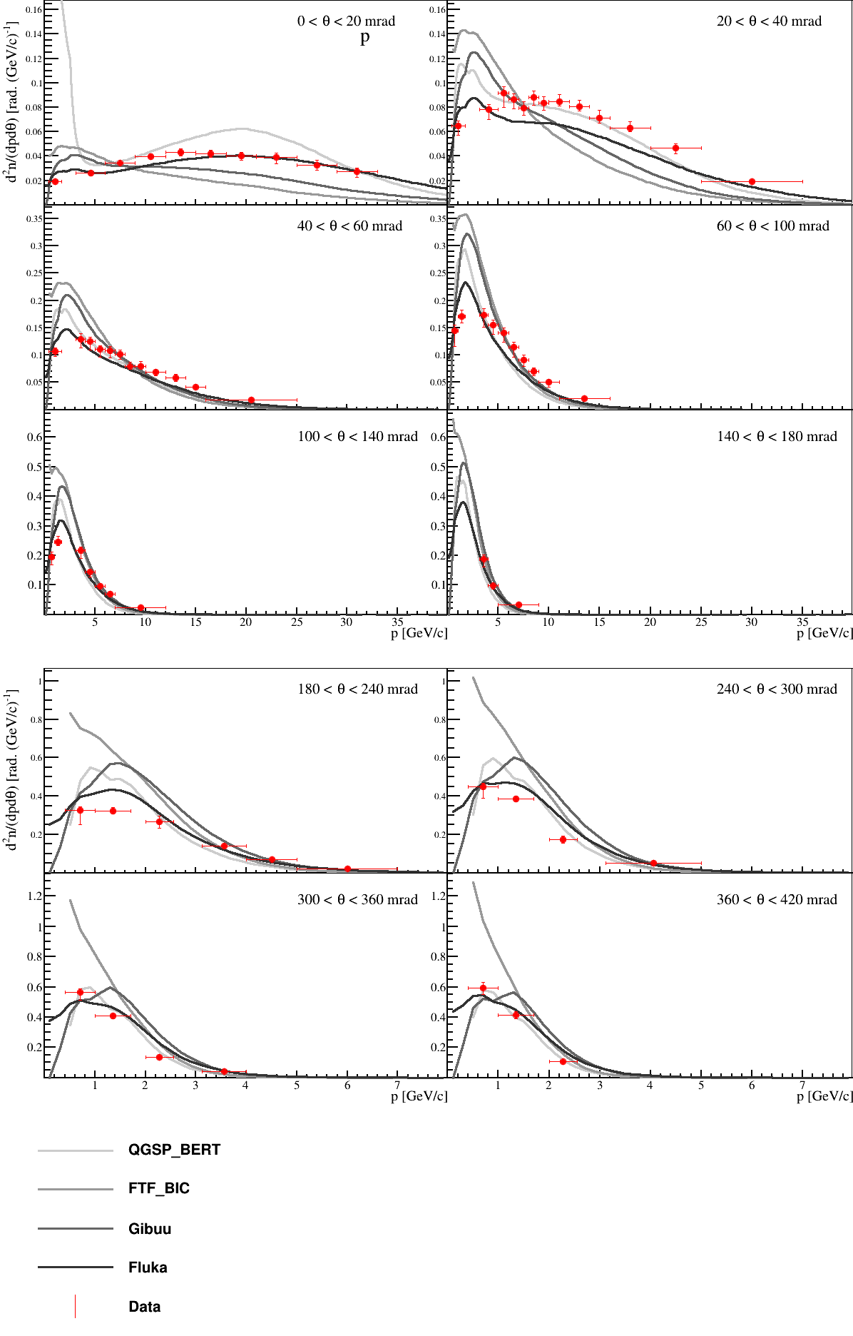
Multiplicity spectra obtained for , and in interactions are presented in Figures 13, 14 and 15. The spectra are shown as 1-dimensional momentum spectra for individual bins of . The error bars represent the total uncertainty except for the normalization uncertainty. The results are compared to the predictions of the GEANT4 physics lists: QGSP_BERT and FTF_BIC as well as GiBUU2019 [26] and FLUKA2011.2x.7 [27, 28, 29]. In general, the spectra fall within the range of predictions of the models used. No single model describes the spectra aptly for the full phase space. The models exhibit a large variability in their predictions of and especially spectra. QGSP_BERT seems to provide the best prediction of spectra, while no single model seems to provide a satisfactory description of spectra. Tables in Ref. [25] present the numerical values of the multiplicity measurements of , and along with statistical, systematic and total uncertainties for each kinematic bin analyzed. The normalization uncertainty of % is not included in the values of the uncertainties shown in these tables but should be attributed to the multiplicity spectra of all hadron species analyzed.


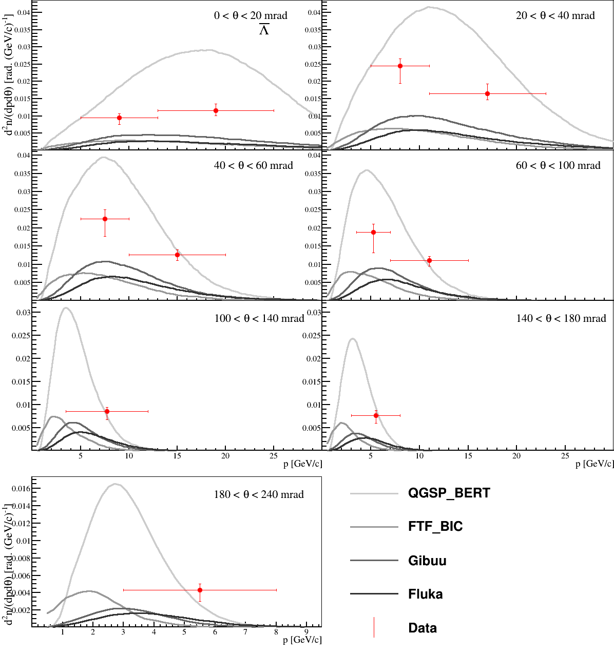
Multiplicity spectra obtained for charged pions, charged kaons and protons in interactions are shown in Figures 16 through 20. The results are compared to the predictions of the GEANT4 physics lists: QGSP_BERT and FTF_BIC as well as GiBUU2019 and FLUKA2011. In general, no single model provides a good description of the charged hadron spectra for all particle species and for the full phase space, but FLUKA2011 seems to provide the best overall description. However, it should be noted that in the first few angular bins, an important region for neutrino beams, FLUKA2011 slightly over-predicts the production of . Tables in Ref. [25] present the numerical values of the multiplicity measurements of charged pions, charged kaons and protons along with statistical, systematic and total uncertainties for each kinematic bin analyzed. The normalization uncertainty of % is not included in the values of the uncertainties shown in these tables but should be attributed to the multiplicity spectra of all hadron species analyzed.
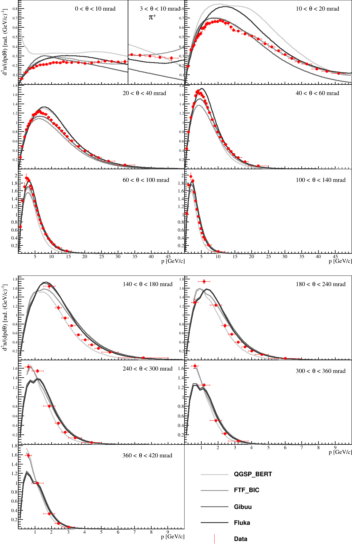
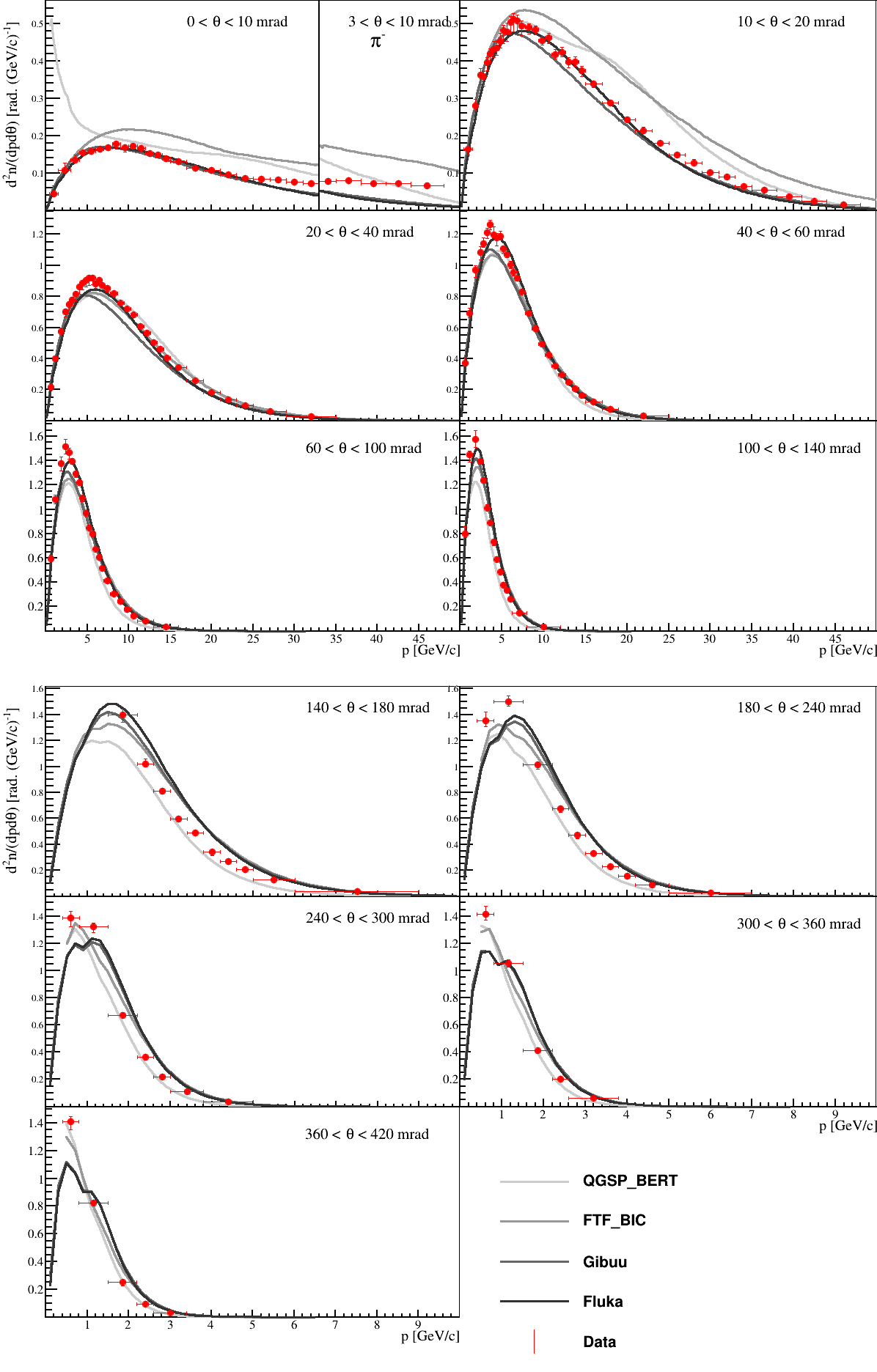
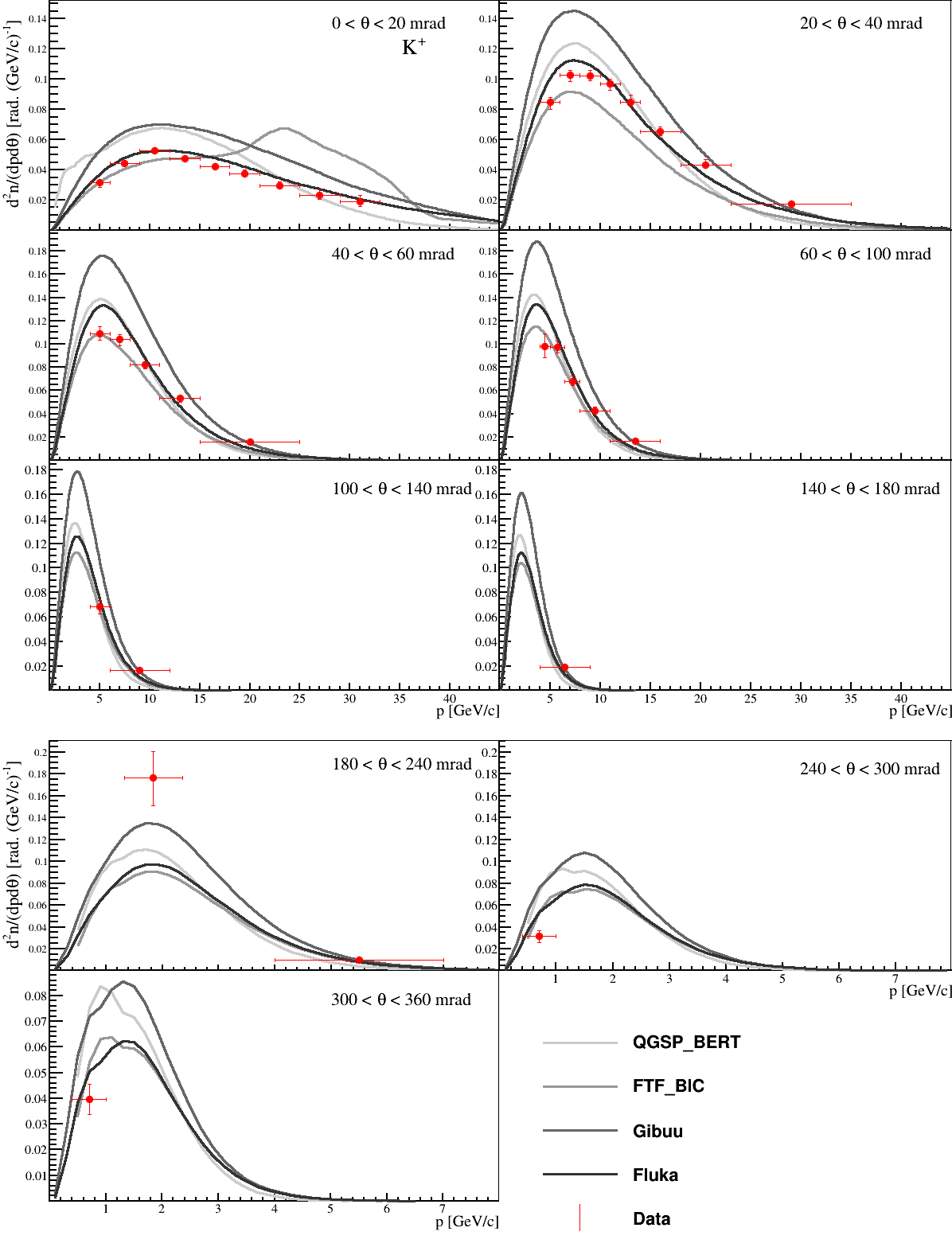

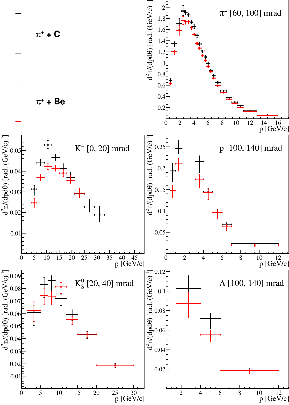
Measurements of spectra of produced , , proton, and from interactions of are shown in comparison to the results for interactions of for representative angular bins in Figure 21. The spectra are largely similar. The most notable difference in the spectra is that the multiplicities tend to be lower in the regions of low momentum and high production angle in interactions of . The full set of comparisons between the spectra results of and is presented in Ref. [25].
9 Summary and Conclusions
In summary, hadron production was studied in interactions of and . For both of these reactions, the integrated production and inelastic cross sections were measured. Furthermore, differential cross sections were measured for produced , , , , protons, , and . The inelastic cross sections measurements are the first to be made at a beam momentum of 60 GeV/. The production cross section of interactions of was measured for the first time as well. The differential cross sections were measured for the first time at this beam momentum scale, and compared to previous measurements at lower beam momenta, a larger kinematic phase space and more particle species were studied. These results will enable neutrino flux predictions to be constrained in neutrino experiments using the NuMI beam and future neutrino beam at LBNF. Specifically, these results can be used to reduce the uncertainties associated with secondary interactions of pions in the carbon targets and the beryllium elements in these beam lines.
Acknowledgments
We would like to thank the CERN EP, BE, HSE and EN Departments for the strong support of NA61/SHINE. We are grateful to the FLUKA team for their help in producing our model comparisons.
This work was supported by the Hungarian Scientific Research Fund (grant NKFIH 123842/123959), the Polish Ministry of Science and Higher Education (grants 667/N-CERN/2010/0, NN 202 48 4339 and NN 202 23 1837), the National Science Centre Poland (grants 2011/03/N/ST2/03691, 2013/11/N/ST2/03879, 2014/13/N/ST2/02565, 2014/14/E/ST2/00018, 2014/15/B/ST2/02537 and 2015/18/M/ST2/00125, 2015/19/N/ST2 /01689, 2016/23/B/ST2/00692, 2017/25/N/ST2/02575, 2018/30 /A /ST2 /00226), the Russian Science Foundation, grant 16-12-10176, the Russian Academy of Science and the Russian Foundation for Basic Research (grants 08-02-00018, 09-02-00664 and 12-02-91503-CERN), the Ministry of Science and Education of the Russian Federation, grant No. 3.3380.2017/4.6, the National Research Nuclear University MEPhI in the framework of the Russian Academic Excellence Project (contract No. 02.a03.21.0005, 27.08.2013), the Ministry of Education, Culture, Sports, Science and Technology, Japan, Grant-in-Aid for Scientific Research (grants 18071005, 19034011, 19740162, 20740160 and 20039012), the German Research Foundation (grant GA 1480/2-2), the Bulgarian Nuclear Regulatory Agency and the Joint Institute for Nuclear Research, Dubna (bilateral contract No. 4799-1-18/20), Bulgarian National Science Fund (grant DN08/11), Ministry of Education and Science of the Republic of Serbia (grant OI171002), Swiss Nationalfonds Foundation (grant 200020117913/1), ETH Research Grant TH-01 07-3 and the U.S. Department of Energy.
References
- [1] N. Abgrall et al., [NA61 Collab.] JINST 9 (2014) P06005, arXiv:1401.4699 [physics.ins-det].
- [2] N. Abgrall et al., [NA61/SHINE Collab.] Phys. Rev. C84 (2011) 034604, arXiv:1102.0983 [hep-ex].
- [3] N. Abgrall et al., [NA61/SHINE Collab.] Phys. Rev. C 85 (Mar, 2012) 035210.
- [4] N. Abgrall et al., [NA61/SHINE Collab.] Phys. Rev. C 89 (Feb, 2014) 025205.
- [5] N. Abgrall et al., [NA61/SHINE Collab.] Eur. Phys. J. C76 no. 2, (2016) 84, arXiv:1510.02703 [hep-ex].
- [6] K. Anderson et al., “The NuMI Facility Technical Design Report.” Fermilab-design-1998-01, fermilab-tm-2406, 1998.
- [7] R. Acciarri et al., [DUNE Collab.] arXiv:1512.06148 [physics.ins-det].
- [8] B. Abi et al., [DUNE Collab.] arXiv:1807.10334 [physics.ins-det].
- [9] H. Schellman, [DUNE/LBNF Collab.], “The LBNF Neutrino Beam,” in talk at the 39th International Conference on High Energy Physics (ICHEP2018), Seoul, Korea. 2018.
- [10] A. Bashyal, [DUNE Collab.], “Neutrino Flux Prediction for DUNE,” in talk at the 11th International Workshop on Neutrino-Nucleus Scattering in the Few-GeV Region (NuINT2017), Toronto, Canada. 2017.
- [11] L. Fields, “LBNF Hadron Production Needs and Plans,” in talk at the NA61/SHINE Beyond 2020 Workshop, Geneva, Switzerland. 2017.
- [12] C. Alt et al., [NA49 Collab.] Eur. Phys. J. C49 (2007) 897–917, arXiv:hep-ex/0606028 [hep-ex].
- [13] M. G. Catanesi et al., [HARP Collab.] Astropart. Phys. 29 (2008) 257–281, arXiv:0802.0657 [astro-ph].
- [14] C. Bovet, S. Milner, and A. Placci IEEE Trans. Nucl. Sci. 25 (1978) 572–576.
- [15] C. Bovet, R. Maleyran, L. Piemontese, A. Placci, and M. Placidi CERN-82-13, CERN-YELLOW-82-13 (1982) .
- [16] A. Aduszkiewicz et al., [NA61/SHINE Collab.] Phys. Rev. D98 no. 5, (2018) 052001, arXiv:1805.04546 [hep-ex].
- [17] S. Agostinelli et al., [GEANT4 Collab.] Nucl. Instrum. Meth. A506 (2003) 250–303.
- [18] J. Allison et al. IEEE Trans. Nucl. Sci. 53 (2006) 270.
- [19] J. Allison et al. Nucl. Instrum. Meth. A835 (2016) 186–225.
- [20] N. Charitonidis, “Muon Population in NA61.” https://edms.cern.ch/ui/file/1909492/1/Muons_NA61.pdf, Feb, 2018. CERN-EDMS-1909492.
- [21] N. Charitonidis, “Positron Population in NA61,” 2019. Private communication.
- [22] A. Carroll et al. Phys. Lett. B80 (1979) 319.
- [23] S. P. Denisov, S. V. Donskov, Yu. P. Gorin, R. N. Krasnokutsky, A. I. Petrukhin, Yu. D. Prokoshkin, and D. A. Stoyanova Nucl. Phys. B61 (1973) 62–76.
- [24] M. Tanabashi et al., [Particle Data Group Collab.] Phys. Rev. D 98 (Aug, 2018) 030001.
- [25] S. R. Johnson et al., “Tables with numerical results for paper on hadron production from 2016 pion data.” https://edms.cern.ch/document/2215444, 2019. CERN-EDMS-2215444.
- [26] O. Buss, T. Gaitanos, K. Gallmeister, H. van Hees, M. Kaskulov, O. Lalakulich, A. B. Larionov, T. Leitner, J. Weil, and U. Mosel Phys. Rept. 512 (2012) 1–124, arXiv:1106.1344 [hep-ph].
- [27] G. Battistoni et al., “Overview of the FLUKA code,” 2015.
- [28] T. T. Bohlen, F. Cerutti, M. P. W. Chin, A. Fasso, A. Ferrari, P. G. Ortega, A. Mairani, P. R. Sala, G. Smirnov, and V. Vlachoudis Nucl. Data Sheets 120 (2014) 211–214.
- [29] A. Ferrari, P. R. Sala, A. Fasso, and J. Ranft, “FLUKA: A multi-particle transport code,” 2005.