跳到论文正文
W Papers独立论文阅读器 arXiv:1909.06222 论文正文 计算阅读时间 · 0%
引用这篇论文根据当前论文元数据生成,正式投稿前建议核对。


License: arXiv.org perpetual non-exclusive license
arXiv:1909.06222v1 [math.FA] 11 Sep 2019

The NC-Proximal Average for Multiple Functions Thanks: Research by these authors was supported by UBC UGF and by NSERC of Canada.

W. Hare Thanks: Mathematics, University of British Columbia, Kelowna. warren.hare@ubc.ca    C. Planiden Thanks: Mathematics, University of British Columbia, Kelowna. chayneplaniden@hotmail.com
January 15, 2014
Abstract

The NC-proximal average is a parametrized function used to continuously transform one proper, lsc, prox-bounded function into another. Until now it has been defined for two functions. The purpose of this article is to redefine it so that any finite number of functions may be used. The layout generally follows that of [11], extending those results to the more general case and in some instances giving alternate proofs by using techniques developed after the publication of that paper. We conclude with an example examining the discontinuity of the minimizers of the NC-proximal average.

Keywords: Proximal average, prox-regularity, Moreau envelope, minima

1 Introduction

In 2008, Bauschke, Lucet, and Trienis, first addressed the question of how to transform one convex function into another in a continuous manner [2]. Given proper convex functions f0f_{0} and f1f_{1}, their proposed solution, the proximal average, used Fenchel conjugates to define a parameterized function P​A​(x,λ)PA(x,\lambda) such that P​APA is epi-continuous with respect to λ,\lambda, and P​A​(x,0)=f0​(x)PA(x,0)=f_{0}(x), P​A​(x,1)=f1​(x)PA(x,1)=f_{1}(x) for all x.x. The proximal average has been studied extensively since its original conception, and many favourable properties and applications of this approach have arisen [1, 3, 4, 6, 7, 8, 10, 9, 11, 14, 15, 16, 18]. For example, the minimizers of the proximal average function change continuously with respect to λ\lambda [10].

The proximal average has also been generalized and reformulated in a number of useful manners. For example, in [1], the proximal average is generalized to a finite number of convex functions. In [5], the proximal average is generalized to allow for alternate kernels, which further allowed for applications with monotone operators. In [9], the proximal average is reformulated to apply to saddle functions. And, in [11], the proximal average was reformulated to work with two (nonconvex), proper, lsc, prox-bounded functions. This document generalizes the work done in [11] to allow for a finite number of such functions.

Given two proper, lsc, prox-bounded functions, f0f_{0} and f1f_{1}, the NC-proximal average was originally defined as

P​Ar​(x,λ):=−er+λ⁡(1−λ)​(−(1−λ)​er​f0−λ​er​f1)​(x)PA_{r}(x,\lambda):=-e_{r+\lambda(1-\lambda)}\left(-(1-\lambda)e_{r}f_{0}-\lambda e_{r}f_{1}\right)(x)

where λ∈[0,1]\lambda\in[0,1] and er​fe_{r}f is the Moreau envelope of ff using the prox-parameter r,r, defined as

er​f​(x):=infy{f⁡(y)+r2​|y−x|2}.e_{r}f(x):=\inf\limits_{y}\left\{f(y)+\frac{r}{2}|y-x|^{2}\right\}.

Associated with the Moreau envelope, and closely related to the NC-proximal average, is the proximal point mapping Pr​fP_{r}f defined as

Pr​f​(x):=argminy{f⁡(y)+r2​|y−x|2}.P_{r}f(x):=\operatornamewithlimits{argmin}\limits_{y}\left\{f(y)+\frac{r}{2}|y-x|^{2}\right\}.

In [11] the function P​ArPA_{r} is analyzed and a number of propositions and theorems are developed in order to describe its properties. Here, we extend those results for a finite number of proper, lsc, prox-bounded functions fif_{i}, i∈{1,2,…,m}.i\in\{1,2,\ldots,m\}. We begin by defining the NC-proximal average as

PAr,δ(x,λ):=−er+δ⁡(λ)(−∑i=1mλierfi)(x),PA_{r,\delta}(x,\lambda):=-e_{r+\delta(\lambda)}\left(-\sum\limits_{i=1}^{m}\lambda_{i}e_{r}f_{i}\right)(x), (1.1)
λ∈Λ:={(λ1,λ2,…,λm)∈ℝm:λi≥0​ for all ​i​ and ​∑i=1mλi=1},\lambda\in\Lambda:=\left\{(\lambda_{1},\lambda_{2},\ldots,\lambda_{m})\in\mathbb{R}^{m}:\lambda_{i}\geq 0\mbox{ for all }i\mbox{ and }\sum\limits_{i=1}^{m}\lambda_{i}=1\right\},

and δ\delta is any continuous function such that δ⁡(λ)=0\delta(\lambda)=0 if λ=ei\lambda=e_{i} (the canonical unit vector whose it​hi^{th} component is 1) for some i,i, and δ⁡(λ)>0\delta(\lambda)>0 otherwise. This definition generalizes that of [11] in two respects. First, the original definition is restricted to outer prox-parameter r+λ⁡(1−λ),r+\lambda(1-\lambda), when in fact the λ⁡(1−λ)\lambda(1-\lambda) term can be replaced by any function δ\delta as described above. Second, the results found in [11] are reworked in order to accommodate any finite number of functions.

Remark 1.1.

It should be clear that the choice of the function δ\delta used in defining the NC-proximal average will have a great impact on the parameterized function P​Ar,δPA_{r,\delta}. However, it will become clear in this paper that the underlying properties of P​Ar,δPA_{r,\delta} are in fact not effected by δ\delta. As such, for ease of notation, except when necessary we shall simplify P​Ar,δPA_{r,\delta} to P​ArPA_{r}.

The remainder of this article is organized as follows. Section 2 provides definitions and shows that P​ArPA_{r} is well-defined. Section 3 explores the prox-regularity and para-prox-regularity aspects of the function, and Section 4 considers its stability. We conclude, in Section 5, with some discussion on the minimizers of the NC-proximal average, including an example that demonstrates that the minimizers of the NC-proximal average may be multi-valued and discontinuous.

2 Preliminaries

Throughout this paper, we use qq to represent the norm-squared function, q⁡(x)=|x|2q(x)=|x|^{2}. This section restates some definitions we need, and shows that under basic assumptions, P​ArPA_{r} is a well-defined function.

Definition 2.1.

A proper function f:ℝn→ℝ∪{∞}f:\mathbb{R}^{n}\rightarrow\mathbb{R}\cup\{\infty\} is said to be prox-bounded if there exist r>0r>0 and a point x¯\bar{x} such that er​f​(x¯)>−∞.e_{r}f(\bar{x})>-\infty. The infimum of the set of all such rr is called the threshold of prox-boundedness.

Definition 2.2.

A function is lower-𝒞2\mathcal{C}^{2} on an open set VV if it is finite-valued on VV and at any point x∈Vx\in V the function appended with a quadratic term is convex on some open convex neighborhood V′V^{\prime} of x.x. The function is said to be lower-𝒞2\mathcal{C}^{2} (with no mention of VV) if V=ℝn.V=\mathbb{R}^{n}.

Our first task is to confirm that P​ArPA_{r} is a well-defined and well-behaved function. The following proposition generalizes [11, Prop 2.5].

Proposition 2.3.

For i∈{1,2,…,m}i\in\{1,2,\ldots,m\} let fi:ℝn→ℝ∪{∞}f_{i}:\mathbb{R}^{n}\rightarrow\mathbb{R}\cup\{\infty\} be proper, lsc, prox-bounded functions with respective thresholds r¯i\bar{r}_{i}. Let r>maxi⁡{r¯i}.r>\max\limits_{i}\{\bar{r}_{i}\}. Then for all λ∈Λ\lambda\in\Lambda, P​ArPA_{r} is a proper function in xx. Furthermore, if λi≠1\lambda_{i}\neq 1 for all ii, then P​ArPA_{r} defines a lower-𝒞2\mathcal{C}^{2} function in xx. Finally, if for some ii one has that fi+r2​qf_{i}+\frac{r}{2}q is convex, then P​Ar​(⋅,ei)=fi.PA_{r}(\cdot,e_{i})=f_{i}.

Proof: We know that −er​fi-e_{r}f_{i} is well-defined for all ii, since r>r¯ir>\bar{r}_{i} for all ii. By [11, Lem 2.4], which is extendible to the case of mm functions, we know that −∑i=1mλierfi-\sum\limits_{i=1}^{m}\lambda_{i}e_{r}f_{i} is a proper, lower-𝒞2\mathcal{C}^{2}, prox-bounded function, with threshold r¯≤∑i=1mλi​r=r\bar{r}\leq\sum\limits_{i=1}^{m}\lambda_{i}r=r. Thus the Moreau envelope of −∑i=1mλierfi-\sum\limits_{i=1}^{m}\lambda_{i}e_{r}f_{i} is well-defined and proper whenever the prox-parameter is greater than or equal to rr (as is the case when λ∈Λ\lambda\in\Lambda), and it is lower-𝒞2\mathcal{C}^{2} whenever the prox-parameter is strictly greater than rr (as is the case when λ∈Λ\lambda\in\Lambda and λi≠1\lambda_{i}\neq 1 for all ii). The last statement is proved by applying [17, Ex 11.26 (d)] to P​Ar​(x,ei)=−er​(−er​fi)​(x)PA_{r}(x,e_{i})=-e_{r}(-e_{r}f_{i})(x).∎

3 Prox-Regularity

In this section, we wish to establish the conditions under which the function ∑i=1mλi​er​fi\sum\limits_{i=1}^{m}\lambda_{i}e_{r}f_{i} is para-prox-regular, so that in Section 4 we may explore the stability of P​Ar.PA_{r}. Let us recall what we mean by prox-regularity and para-prox-regularity of a function.

Definition 3.1.

A proper function ff is prox-regular at a point x¯\bar{x} for v¯∈∂f⁡(x¯)\bar{v}\in\partial f(\bar{x}) if ff is locally lsc at x¯\bar{x} and there exist ϵ>0\epsilon>0 and r>0r>0 such that

f⁡(x′)≥f⁡(x)+⟨v,x′−x⟩−r2​|x′−x|2f(x^{\prime})\geq f(x)+\langle v,x^{\prime}-x\rangle-\frac{r}{2}|x^{\prime}-x|^{2} (3.1)

whenever x′≠x,x^{\prime}\neq x, |x′−x¯|<ϵ,|x^{\prime}-\bar{x}|<\epsilon, |x−x¯|<ϵ,|x-\bar{x}|<\epsilon, |f⁡(x)−f⁡(x¯)|<ϵ,|f(x)-f(\bar{x})|<\epsilon, v∈∂f⁡(x),v\in\partial f(x), and |v−v¯|<ϵ.|v-\bar{v}|<\epsilon. We say the function is continuously prox-regular at x¯\bar{x} for v¯\bar{v} if, in addition, ff is continuous as a function of (x,v)∈gph∂f(x,v)\in\operatorname{gph}\partial f at (x¯,v¯).(\bar{x},\bar{v}). The function is said to be prox-regular at x¯\bar{x} (with no mention of v¯\bar{v}) if it is prox-regular at x¯\bar{x} for every v¯∈∂f⁡(x¯),\bar{v}\in\partial f(\bar{x}), and simply prox-regular (with no mention of x¯\bar{x}) if it is prox-regular at x¯\bar{x} for every x¯∈dom⁡f.\bar{x}\in\operatorname{dom}f.

From a graphical point of view, a prox-regular function is one that is locally bounded below by quadratics of equal curvature. Para-prox-regularity is an extension of this idea that includes an extra parameter λ\lambda.

Definition 3.2.

A proper, lsc function f:ℝn×ℝs→ℝ∪{∞}f:\mathbb{R}^{n}\times\mathbb{R}^{s}\rightarrow\mathbb{R}\cup\{\infty\} is parametrically prox-regular in xx at x¯\bar{x} for v¯∈∂xf⁡(x¯,λ¯)\bar{v}\in\partial_{x}f(\bar{x},\bar{\lambda}) with compatible parametrization by λ\lambda at λ¯\bar{\lambda} (also refered to as para-prox-regular in xx at (x¯,λ¯)(\bar{x},\bar{\lambda}) for v¯\bar{v}), with parameters ϵ>0\epsilon>0 and r>0,r>0, if

f⁡(x′,λ)≥f⁡(x,λ)+⟨v,x′−x⟩−r2​|x′−x|2f(x^{\prime},\lambda)\geq f(x,\lambda)+\langle v,x^{\prime}-x\rangle-\frac{r}{2}|x^{\prime}-x|^{2} (3.2)

whenever x′≠x,x^{\prime}\neq x, |x′−x¯|<ϵ,|x^{\prime}-\bar{x}|<\epsilon, |x−x¯|<ϵ,|x-\bar{x}|<\epsilon, |f⁡(x,λ)−f⁡(x¯,λ¯)|<ϵ,|f(x,\lambda)-f(\bar{x},\bar{\lambda})|<\epsilon, |λ−λ¯|<ϵ,|\lambda-\bar{\lambda}|<\epsilon, v∈∂xf⁡(x,λ),v\in\partial_{x}f(x,\lambda), and |v−v¯|<ϵ.|v-\bar{v}|<\epsilon. It is continuously para-prox-regular in xx at (x¯,λ¯)(\bar{x},\bar{\lambda}) for v¯\bar{v} if, in addition, ff is continuous as a function of (x,λ,v)∈gph∂xf(x,\lambda,v)\in\operatorname{gph}\partial_{x}f at (x¯,λ¯,v¯).(\bar{x},\bar{\lambda},\bar{v}). If the parameter λ¯,\bar{\lambda}, the subgradient v¯,\bar{v}, or the point x¯\bar{x} is omitted, then the para-prox-regularity of ff is understood to mean for all λ¯∈dom⁡f⁡(x¯,⋅),\bar{\lambda}\in\operatorname{dom}f(\bar{x},\cdot), for all v¯∈∂xf⁡(x¯,λ¯),\bar{v}\in\partial_{x}f(\bar{x},\bar{\lambda}), or for all x¯∈dom⁡f⁡(⋅,λ¯),\bar{x}\in\operatorname{dom}f(\cdot,\bar{\lambda}), respectively.

Proposition 3.3.

For i∈{1,2,…,m}i\in\{1,2,\ldots,m\} let fi:ℝn→ℝ∪{∞}f_{i}:\mathbb{R}^{n}\rightarrow\mathbb{R}\cup\{\infty\} be proper, lsc, and prox-bounded with threshold ri.r_{i}. Let r>rir>r_{i} for all i.i. Define

F⁡(x,λ)={−∑i=1mλierfi(x),λ∈Λ∞,λ∉Λ.F(x,\lambda)=\begin{cases}-\sum\limits_{i=1}^{m}\lambda_{i}e_{r}f_{i}(x)&,\penalty\ \lambda\in\Lambda\\ \infty&,\penalty\ \lambda\not\in\Lambda.\end{cases}

Then FF is continuously para-prox-regular at any x¯\bar{x}, with compatible parametrization by λ\lambda at any λ¯∈Λ.\bar{\lambda}\in\Lambda. Moreover, FF is lower-𝒞2\mathcal{C}^{2} and strictly continuous, and if (0,y)∈∂∞F⁡(x¯,λ¯)(0,y)\in\partial^{\infty}F(\bar{x},\bar{\lambda}) then y=0.y=0.

Proof: Since fif_{i} is proper, lsc and prox-bounded for all i,i, [17, Ex 10.32] gives us that −er​fi-e_{r}f_{i} is lower-𝒞2\mathcal{C}^{2} for all i.i. The sum of lower-𝒞2\mathcal{C}^{2} functions is lower-𝒞2,\mathcal{C}^{2}, and any lower-𝒞2\mathcal{C}^{2} function is strictly continuous [17, Thm 10.31], so FF is lower-𝒞2\mathcal{C}^{2} and strictly continuous. Finally, [17, Thm 9.31] states that strict continuity of FF at (x¯,λ¯)(\bar{x},\bar{\lambda}) is equivalent to ∂∞F⁡(x¯,λ¯)={0},\partial^{\infty}F(\bar{x},\bar{\lambda})=\{0\}, which gives us that (0,y)∈∂∞F⁡(x¯,λ¯)⇒y=0.(0,y)\in\partial^{\infty}F(\bar{x},\bar{\lambda})\Rightarrow y=0. This gives us all the conditions of [12, Thm 5.7], and its conclusion is the result we seek.∎

Remark 3.4.

The proof of [11, Lemma 3.3] can also be adapted for a longer, but more direct proof of Proposition 3.3.

4 Stability

We are now ready to explore the stability of the NC-proximal average. By Proposition 3.3, we can see that P​ArPA_{r} is the Moreau envelope of a para-prox-regular function. This allows us to take advantage of the work done in [13], where the tilt stability and full stability of Moreau envelopes and proximal mappings of para-prox-regular functions was studied.

Theorem 4.1.

[13, Thm 4.6] Let F:ℝn×ℝs→ℝ∪{∞}F:\mathbb{R}^{n}\times\mathbb{R}^{s}\rightarrow\mathbb{R}\cup\{\infty\} be proper, lsc, and continuously para-prox-regular at (x¯,λ¯)(\bar{x},\bar{\lambda}) for v¯∈∂xF⁡(x¯,λ¯),\bar{v}\in\partial_{x}F(\bar{x},\bar{\lambda}), with parameters ϵ\epsilon and r.r. Assume further that FF is prox-bounded with threshold ρ,\rho, and that FF satisfies the following:

  1. 1.

    (0,y)∈∂∞F⁡(x¯,λ¯)⇒y=0,(0,y)\in\partial^{\infty}F(\bar{x},\bar{\lambda})\Rightarrow y=0,

  2. 2.

    (0,λ′)∈D∗​(∂xF)​(x¯,λ¯|v¯)​(0)⇒λ′=0,(0,\lambda^{\prime})\in D^{*}(\partial_{x}F)(\bar{x},\bar{\lambda}|\bar{v})(0)\Rightarrow\lambda^{\prime}=0,

  3. 3.

    (x′,λ′)∈D∗​(∂xF)​(x¯,λ¯|v¯)​(v′),v′≠0⇒⟨x′,v′⟩>−ρ′​|v′|2(x^{\prime},\lambda^{\prime})\in D^{*}(\partial_{x}F)(\bar{x},\bar{\lambda}|\bar{v})(v^{\prime}),v^{\prime}\neq 0\Rightarrow\langle x^{\prime},v^{\prime}\rangle>-\rho^{\prime}|v^{\prime}|^{2} for some ρ′>0,\rho^{\prime}>0,

  4. 4.

    ∂xF⁡(x¯,⋅)\partial_{x}F(\bar{x},\cdot) has a continuous selection gg near λ¯,\bar{\lambda}, with g⁡(λ¯)=v¯.g(\bar{\lambda})=\bar{v}.

If r¯>max⁡{ρ,ρ′,r}\bar{r}>\max\{\rho,\rho^{\prime},r\}, then there exist K>0K>0 and a neighborhood ℬ=Bδ​(x¯+v¯r,λ¯,r¯)\mathcal{B}=B_{\delta}(\bar{x}+\frac{\bar{v}}{r},\bar{\lambda},\bar{r}) such that for all (x,λ,r),(x′,λ′,r′)∈ℬ(x,\lambda,r),(x^{\prime},\lambda^{\prime},r^{\prime})\in\mathcal{B} we have that Pr​Fλ​(x)P_{r}F_{\lambda}(x) and Pr′​Fλ′​(x′)P_{r^{\prime}}F_{\lambda^{\prime}}(x^{\prime}) are single-valued, with

|PrFλ(x)−Pr′Fλ′(x′)|≤K|r(x−x¯)−r′(x′−x¯),λ−λ′,r−r′)|,|P_{r}F_{\lambda}(x)-P_{r^{\prime}}F_{\lambda^{\prime}}(x^{\prime})|\leq K|r(x-\bar{x})-r^{\prime}(x^{\prime}-\bar{x}),\lambda-\lambda^{\prime},r-r^{\prime})|,

where Fλ​(x)=F⁡(x,λ).F_{\lambda}(x)=F(x,\lambda).

Lemma 4.2.

[11, Lem 4.4] Suppose the function H:ℝn×ℝs→ℝ∪{∞}H:\mathbb{R}^{n}\times\mathbb{R}^{s}\rightarrow\mathbb{R}\cup\{\infty\} is finite, single-valued, and Lipschitz continuous in (x,λ)(x,\lambda) near (x¯,λ¯)(\bar{x},\bar{\lambda}) with local Lipschitz constant Lip⁡H.\operatorname{Lip}H. Then

(0,λ′)∈D∗​H​(x¯,λ¯|H⁡(x¯,λ¯))​(0)⇒λ′=0,(0,\lambda^{\prime})\in D^{*}H(\bar{x},\bar{\lambda}|H(\bar{x},\bar{\lambda}))(0)\Rightarrow\lambda^{\prime}=0,

and for ρ>Lip⁡H\rho>\operatorname{Lip}H one has

(x′,λ′)∈D∗​H​(x¯,λ¯|H⁡(x¯,λ¯))​(v′),v′≠0⇒⟨x′,v′⟩>−ρ​|v′|2.(x^{\prime},\lambda^{\prime})\in D^{*}H(\bar{x},\bar{\lambda}|H(\bar{x},\bar{\lambda}))(v^{\prime}),v^{\prime}\neq 0\Rightarrow\langle x^{\prime},v^{\prime}\rangle>-\rho|v^{\prime}|^{2}.

The next proposition is an analog of [11, Prop 4.5], rewritten to work with a finite number of functions. The proof of [11, Prop 4.5] is easily adaptable to this setting, so we present only the key details.

Proposition 4.3.

For i∈{1,2,…,m}i\in\{1,2,\ldots,m\}, let fi:ℝn→ℝ∪{∞}f_{i}:\mathbb{R}^{n}\rightarrow\mathbb{R}\cup\{\infty\} be proper, lsc, and prox-bounded with threshold ri.r_{i}. Let r>maxi⁡{ri},r>\max\limits_{i}\{r_{i}\}, and define

F(x,λ):=−∑i=1mλierfi(x).F(x,\lambda):=-\sum\limits_{i=1}^{m}\lambda_{i}e_{r}f_{i}(x).

If Pr​fiP_{r}f_{i} is single-valued and Lipschitz continuous for all i,i, then the following three properties hold:

  1. 1.

    (0,λ′)∈D∗​(∂xF)​(x¯,λ¯|v¯)​(0)⇒λ′=0,(0,\lambda^{\prime})\in D^{*}(\partial_{x}F)(\bar{x},\bar{\lambda}|\bar{v})(0)\Rightarrow\lambda^{\prime}=0,

  2. 2.

    for some ρ>0\rho>0 we have (x′,λ′)∈D∗(∂xF(x¯,λ¯|v¯)(v′),v′≠0⇒⟨x′,v′⟩>−ρ|v′|2,(x^{\prime},\lambda^{\prime})\in D^{*}(\partial_{x}F(\bar{x},\bar{\lambda}|\bar{v})(v^{\prime}),v^{\prime}\neq 0\Rightarrow\langle x^{\prime},v^{\prime}\rangle>-\rho|v^{\prime}|^{2}, and

  3. 3.

    the set-valued mapping ∂xF⁡(x¯,⋅)\partial_{x}F(\bar{x},\cdot) has a continuous selection gg near λ¯.\bar{\lambda}.

Proof: Since Pr​fiP_{r}f_{i} is Lipschitz continuous, we have that er​fi∈𝒞1+e_{r}f_{i}\in\mathcal{C}^{1+} with ∇erfi=r(I−Prfi)\nabla e_{r}f_{i}=r(I-P_{r}f_{i}) [13, Thm 2.4]. Hence,

∂xF⁡(x¯,λ)\displaystyle\partial_{x}F(\bar{x},\lambda) =∇x(−∑i=1mλierfi)(x¯,λ)\displaystyle=\nabla_{x}(-\sum\limits_{i=1}^{m}\lambda_{i}e_{r}f_{i})(\bar{x},\lambda)
=r⁡[(∑i=1mλi​Pr​fi​(x¯))−x¯]\displaystyle=r\left[\left(\sum\limits_{i=1}^{m}\lambda_{i}P_{r}f_{i}(\bar{x})\right)-\bar{x}\right]

which is linear in λ,\lambda, showing Property 3. Since Pr​fiP_{r}f_{i} is single-valued and Lipschitz continuous, we have ∂xF⁡(x,λ)\partial_{x}F(x,\lambda) single-valued and Lipschitz continuous. Properties 1 and 2 follow by applying Lemma 4.2.∎

Proposition 4.4.

For i∈{1,2,…,m}i\in\{1,2,\ldots,m\}, let fi:ℝn→ℝ∪{∞}f_{i}:\mathbb{R}^{n}\rightarrow\mathbb{R}\cup\{\infty\} be proper, lsc, and prox-bounded with threshold ri.r_{i}. Let r>maxi⁡{ri}.r>\max\limits_{i}\{r_{i}\}. Then PAr(⋅,λ)+r+δ⁡(λ)2q(⋅−x¯)PA_{r}(\cdot,\lambda)+\frac{r+\delta(\lambda)}{2}q(\cdot-\bar{x}) is convex for any x¯.\bar{x}. Hence, P​Ar​(⋅,λ)PA_{r}(\cdot,\lambda) is lower-𝒞2.\mathcal{C}^{2}.

Proof: Define Fλ:=−∑i=1mλierfi.F_{\lambda}:=-\sum\limits_{i=1}^{m}\lambda_{i}e_{r}f_{i}. Then

P​Ar+r+δ⁡(λ)2​q=−er+δ⁡(λ)​(Fλ)+r+δ⁡(λ)2​q.PA_{r}+\frac{r+\delta(\lambda)}{2}q=-e_{r+\delta(\lambda)}(F_{\lambda})+\frac{r+\delta(\lambda)}{2}q.

By [17, Ex 11.26], we have

−er+δ⁡(λ)(Fλ)+r+δ⁡(λ)2q=(Fλ+r+δ⁡(λ)2q)∗((r+δ(λ))⋅),-e_{r+\delta(\lambda)}(F_{\lambda})+\frac{r+\delta(\lambda)}{2}q=\left(F_{\lambda}+\frac{r+\delta(\lambda)}{2}q\right)^{*}((r+\delta(\lambda))\cdot),

where f∗​(x):=supy{⟨x,y⟩−f⁡(y)}f^{*}(x):=\sup_{y}\{\langle x,y\rangle-f(y)\} is the Fenchel conjugate as defined in [2]. This is an affine function composed with a convex function (as conjugate functions are convex), and as such it is convex. Notice that shifting the argument of qq by x¯\bar{x} only results in the addition of a linear term, as

q⁡(x−x¯)=q⁡(x)+2​⟨x,x¯⟩+q⁡(x¯)q(x-\bar{x})=q(x)+2\langle x,\bar{x}\rangle+q(\bar{x})

where q⁡(x¯)q(\bar{x}) is constant and 2​⟨x,x¯⟩2\langle x,\bar{x}\rangle is linear. Hence, PAr+q(⋅−x¯)PA_{r}+q(\cdot-\bar{x}) is convex.∎

Theorem 4.5.

[Stability of P​ArPA_{r}] For i∈{1,2,…,m}i\in\{1,2,\ldots,m\}, let fi:ℝn→ℝ∪{∞}f_{i}:\mathbb{R}^{n}\rightarrow\mathbb{R}\cup\{\infty\} be proper, lsc, and prox-bounded with threshold ri.r_{i}. Let r¯>maxi⁡{ri}\bar{r}>\max\limits_{i}\{r_{i}\} and r¯>ρ′\bar{r}>\rho^{\prime} from Theorem 4.1 Condition 3. Suppose that for all i,i, Pr¯​fiP_{\bar{r}}f_{i} is single-valued and Lipschitz continuous (as is the case when fif_{i} is prox-regular). Then P​Ar¯PA_{\bar{r}} is well-defined and lower-𝒞2.\mathcal{C}^{2}. If in addition

Lip⁡(∑i=1mλi​Pr¯​fi−I)≤1,\operatorname{Lip}\left(\sum\limits_{i=1}^{m}\lambda_{i}P_{\bar{r}}f_{i}-I\right)\leq 1, (4.1)

then for any λ¯\bar{\lambda} such that δ⁡(λ¯)>0\delta(\bar{\lambda})>0 we have

  1. 1.

    P​Ar¯​(⋅,λ¯)∈𝒞1+PA_{\bar{r}}(\cdot,\bar{\lambda})\in\mathcal{C}^{1+} as a function of xx

  2. 2.

    P​Ar¯PA_{\bar{r}} is locally Lipschitz continuous in λ\lambda near λ¯\bar{\lambda}

  3. 3.

    ∇xP​Ar¯\nabla_{x}PA_{\bar{r}} is locally Lipschitz continuous in λ\lambda near λ¯.\bar{\lambda}.

Finally, if fi+r¯2​qf_{i}+\frac{\bar{r}}{2}q is convex then P​Ar¯​(⋅,ei)=fi​(⋅).PA_{\bar{r}}(\cdot,e_{i})=f_{i}(\cdot).

Proof: Let F(x,λ)=−∑i=1mλier¯fi(x).F(x,\lambda)=-\sum\limits_{i=1}^{m}\lambda_{i}e_{\bar{r}}f_{i}(x). By Proposition 2.3, P​Ar¯PA_{\bar{r}} is well-defined and finite-valued. Since Pr¯​fiP_{\bar{r}}f_{i} is single-valued for all i,i, Pr¯​FP_{\bar{r}}F is single-valued as well. Since fif_{i} is proper, lsc, and prox-bounded for all i,i, and r¯\bar{r} is greater than each threshold ri,r_{i}, Proposition 3.3 gives us that FF is continuously para-prox-regular at (x¯,λ¯)(\bar{x},\bar{\lambda}) for v¯∈∂xF⁡(x¯,λ¯),\bar{v}\in\partial_{x}F(\bar{x},\bar{\lambda}), and that (0,y)∈∂∞F⁡(x¯,λ¯)⇒y=0.(0,y)\in\partial^{\infty}F(\bar{x},\bar{\lambda})\Rightarrow y=0. Since Pr¯​fiP_{\bar{r}}f_{i} is single-valued and Lipschitz continuous for all i,i, we have all the conditions of [11, Prop 4.5], and therefore

  1. 1.

    (0,λ′)∈D∗​(∂xF)​(x¯,λ¯|v¯)​(0)⇒λ′=0(0,\lambda^{\prime})\in D^{*}(\partial_{x}F)(\bar{x},\bar{\lambda}|\bar{v})(0)\Rightarrow\lambda^{\prime}=0

  2. 2.

    (x′,λ′)∈D∗​(∂xF)​(x¯,λ¯|v¯)​(v′),v′≠0⇒⟨x′,v′⟩>−ρ​|v′|2(x^{\prime},\lambda^{\prime})\in D^{*}(\partial_{x}F)(\bar{x},\bar{\lambda}|\bar{v})(v^{\prime}),v^{\prime}\neq 0\Rightarrow\langle x^{\prime},v^{\prime}\rangle>-\rho|v^{\prime}|^{2} for some ρ>0\rho>0

  3. 3.

    The mapping ∂xF⁡(x¯,⋅)\partial_{x}F(\bar{x},\cdot) has a continuous selection gg near λ¯.\bar{\lambda}.

Hence the condition r¯>max⁡{ρ,ρ′,r}\bar{r}>\max\{\rho,\rho^{\prime},r\} of Theorem 4.1 is satisfied (recall r=maxi⁡{ri}r=\max_{i}\{r_{i}\}). Therefore, all conditions of Theorem 4.1 hold, and we may assume its result. Since δ∈𝒞2,\delta\in\mathcal{C}^{2}, there exists K¯>0\bar{K}>0 such that

|δ⁡(λ′)−δ⁡(λ)|≤K¯​|λ′−λ||\delta(\lambda^{\prime})-\delta(\lambda)|\leq\bar{K}|\lambda^{\prime}-\lambda|

for all λ′,λ\lambda^{\prime},\lambda near λ¯.\bar{\lambda}. The rest of the proof is the same as that of [11, Thm 4.6].∎

Corollary 4.6.

For i∈{1,2,…,m}i\in\{1,2,\ldots,m\}, let fi:ℝn→ℝ∪{∞}f_{i}:\mathbb{R}^{n}\rightarrow\mathbb{R}\cup\{\infty\} be proper and lsc such that for some r>0,r>0, fi+r2​qf_{i}+\frac{r}{2}q is convex for all i.i. Then fif_{i} is prox-regular and prox-bounded, and inequality (4.1) holds. In particular, all the conditions of Theorem 4.5 hold.

Proof: Since fi+r2​qf_{i}+\frac{r}{2}q is convex for all i,i, we have that fif_{i} is prox-bounded and lower-𝒞2\mathcal{C}^{2}, and therefore prox-regular, for all i.i. Since

P1​(fi+r2​q)=Pr+1​fi,P_{1}(f_{i}+\frac{r}{2}q)=P_{r+1}f_{i},

by [17, Prop 12.19] we have that I−P1​(fi+r2​q)I-P_{1}(f_{i}+\frac{r}{2}q) is Lipschitz continuous with constant at most 1. Thus

Lip⁡{∑i=1mλi​Pr+1​fi−I}=Lip⁡{∑i=1mλi​(I−Pr+1​fi)}≤∑i=1mλ1=1.\operatorname{Lip}\left\{\sum\limits_{i=1}^{m}\lambda_{i}P_{r+1}f_{i}-I\right\}=\operatorname{Lip}\left\{\sum\limits_{i=1}^{m}\lambda_{i}(I-P_{r+1}f_{i})\right\}\leq\sum\limits_{i=1}^{m}\lambda_{1}=1.

This provides inequality (4.1).∎

5 Example

In 2010, Goebel, Hare, and Wang presented a study of the minimizers of the proximal average function for convex functions. For convex functions fif_{i} recall that
−er(−∑i=1mλierfi)(x)-e_{r}\left(-\sum_{i=1}^{m}\lambda_{i}e_{r}f_{i}\right)(x) defined the proximal average from [2]. It was shown that

Φ(λ):=argminx−er(−∑i=1mλierfi)(x)\Phi(\lambda):=\operatornamewithlimits{argmin}_{x}-e_{r}\left(-\sum_{i=1}^{m}\lambda_{i}e_{r}f_{i}\right)(x)

is single-valued and continuous, provided that all functions are bounded below and at least one function is essentially strictly convex [10, Thm 3.8]. We next show that if fif_{i} are convex functions, then the minimizers of the NC-proximal average coincide exactly with the minimizers of the proximal average. In particular, in this case all results from [10] hold.

Lemma 5.1.

For i∈{1,2,…,m}i\in\{1,2,\ldots,m\} let fi:ℝn→ℝ∪{∞}f_{i}:\mathbb{R}^{n}\rightarrow\mathbb{R}\cup\{\infty\} be proper, lsc, convex, and bounded below. Let λ∈Λ\lambda\in\Lambda, then

argminxPAr(x,λ)=argminx∑i=1mλierfi(x)=argminx−er(−∑i=1mλierfi)(x).\operatornamewithlimits{argmin}_{x}PA_{r}(x,\lambda)=\operatornamewithlimits{argmin}_{x}\sum_{i=1}^{m}\lambda_{i}e_{r}f_{i}(x)=\operatornamewithlimits{argmin}_{x}-e_{r}\left(-\sum_{i=1}^{m}\lambda_{i}e_{r}f_{i}\right)(x).

Proof: The minimizers of P​Ar​(⋅,λ)PA_{r}(\cdot,\lambda) coincide with the minimizers of its Moreau envelope er+δ⁡(λ)​P​Ar​(⋅,λ)e_{r+\delta(\lambda)}PA_{r}(\cdot,\lambda). By [17, Ex 11.26(d)], we have that −er+δ⁡(λ)PAr(x,λ)=(∑i=1m−λierfi(x))-e_{r+\delta(\lambda)}PA_{r}(x,\lambda)=\left(\sum_{i=1}^{m}-\lambda_{i}e_{r}f_{i}(x)\right), so the first equality holds. The second equality appears in [10, Lem 3.2].

∎
If fif_{i} are non-convex, then the proximal average is undefined, and the results from [10] no longer apply. In this case, the results of Theorem 4.5 provide some small understanding of the continuity of the minimizers of the NC-proximal average, as follows.

Corollary 5.2.

Let the conditions of Theorem 4.5 hold. Let xk∈argminxP​Ar​(x,λk).x_{k}\in\operatornamewithlimits{argmin}\limits_{x}PA_{r}(x,\lambda_{k}). Suppose λk→λ¯\lambda_{k}\rightarrow\bar{\lambda} and xk→x¯.x_{k}\rightarrow\bar{x}. Then ∇PAr(x¯,λ¯)=0.\nabla PA_{r}(\bar{x},\bar{\lambda})=0.

Proof: By Theorem 4.5, ∇PAr\nabla PA_{r} is Lipschitz continuous in λ.\lambda. Therefore, there exists c>0c>0 such that for all k,k,

|∇PAr(xk,λk)−∇PAr(xk,λ¯)≤c|λk−λ¯|.|\nabla PA_{r}(x_{k},\lambda_{k})-\nabla PA_{r}(x_{k},\bar{\lambda})\leq c|\lambda_{k}-\bar{\lambda}|.

Since xk∈argminPAr(xk,λk),x_{k}\in\operatornamewithlimits{argmin}PA_{r}(x_{k},\lambda_{k}), we know that ∇PAr(xk,λk)=0.\nabla PA_{r}(x_{k},\lambda_{k})=0. So for all k,k,

|∇PAr(xk,λ¯)|≤c|λk−λ¯|.|\nabla PA_{r}(x_{k},\bar{\lambda})|\leq c|\lambda_{k}-\bar{\lambda}|.

Taking the limit as k→∞,k\rightarrow\infty, we find that ∇PAr(x¯,λ¯)=0\nabla PA_{r}(\bar{x},\bar{\lambda})=0.

∎
While Corollary 5.2 gives us a way to identify the minimizers of P​Ar,PA_{r}, it says nothing about the single-valuedness or the continuity of said minimizers. The example that follows illustrates that, in fact, the function of minimizers of the NC-proximal average may be multi-valued and discontinuous.

Let ϵ=12,\epsilon=\frac{1}{2}, and define the functions g0g_{0} and g1g_{1} via

g0​(x):=max⁡{−x,−12​(x−1)2+12,x−2+ϵ},\displaystyle g_{0}(x):=\max\{-x,-\frac{1}{2}(x-1)^{2}+\frac{1}{2},x-2+\epsilon\},
g1​(x):=max⁡{−x+ϵ,−12​(x−1)2+12,x−2}.\displaystyle g_{1}(x):=\max\{-x+\epsilon,-\frac{1}{2}(x-1)^{2}+\frac{1}{2},x-2\}.

Then g0g_{0} and g1g_{1} are proper, lsc, and bounded below.

Refer to caption
Figure 1: Functions g0g_{0} and g1g_{1} for ϵ=0.5.\epsilon=0.5.

Moreover, gi+12​qg_{i}+\frac{1}{2}q is convex for i∈{1,2}i\in\{1,2\}. Let k=2−4−2​ϵ,l=4−2​ϵk=2-\sqrt{4-2\epsilon},\penalty\ l=\sqrt{4-2\epsilon} and define

δ0:=0δ1:=ϵϵ0:=ϵϵ1:=0k0:=0k1:=kl0:=ll1:=2.\begin{array}[]{l l l l}\delta_{0}:=0&\delta_{1}:=\epsilon&\epsilon_{0}:=\epsilon&\epsilon_{1}:=0\\ k_{0}:=0&k_{1}:=k&l_{0}:=l&l_{1}:=2.\end{array}

Consider Pr​gi​(x¯)=argminx{gi​(x)+r2​|x−x¯|2}.P_{r}g_{i}(\bar{x})=\operatornamewithlimits{argmin}\limits_{x}\{g_{i}(x)+\frac{r}{2}|x-\bar{x}|^{2}\}. If r>1r>1, then we find that

Pr​gi​(x¯)={x¯+1r,x¯<ki−1rki,x¯∈[ki−1r,ki−kir+1r]r​x¯−1r−1,x¯∈(ki−kir+1r,li−lir+1r)li,x¯∈[li−lir+1r,li+1r]x¯−1r,x¯>li+1r.P_{r}g_{i}(\bar{x})=\begin{cases}\bar{x}+\frac{1}{r},&\bar{x}<k_{i}-\frac{1}{r}\\ k_{i},&\bar{x}\in[k_{i}-\frac{1}{r},k_{i}-\frac{k_{i}}{r}+\frac{1}{r}]\\ \frac{r\bar{x}-1}{r-1},&\bar{x}\in(k_{i}-\frac{k_{i}}{r}+\frac{1}{r},l_{i}-\frac{l_{i}}{r}+\frac{1}{r})\\ l_{i},&\bar{x}\in[l_{i}-\frac{l_{i}}{r}+\frac{1}{r},l_{i}+\frac{1}{r}]\\ \bar{x}-\frac{1}{r},&\bar{x}>l_{i}+\frac{1}{r}.\end{cases}

Evaluating the Moreau envelope and simplifying, we get

er​gi​(x¯)={−x¯−12​r+δi,x¯<ki−1rr2​x¯2−r​ki​x¯+r−12​ki2+ki,x¯∈[ki−1r,ki−kir+1r]−12​(r−1)​(r​x¯2−2​r​x¯+1),x¯∈(ki−kir+1r,li−lir+1r)r2​x¯2−r​li​x¯+r−12​li2+li,x¯∈[li−lir+1r,li+1r]x¯−2−12​r+ϵi,x¯>li+1r.e_{r}g_{i}(\bar{x})=\begin{cases}-\bar{x}-\frac{1}{2r}+\delta_{i},&\bar{x}<k_{i}-\frac{1}{r}\\ \frac{r}{2}\bar{x}^{2}-rk_{i}\bar{x}+\frac{r-1}{2}k_{i}^{2}+k_{i},&\bar{x}\in[k_{i}-\frac{1}{r},k_{i}-\frac{k_{i}}{r}+\frac{1}{r}]\\ -\frac{1}{2(r-1)}(r\bar{x}^{2}-2r\bar{x}+1),&\bar{x}\in(k_{i}-\frac{k_{i}}{r}+\frac{1}{r},l_{i}-\frac{l_{i}}{r}+\frac{1}{r})\\ \frac{r}{2}\bar{x}^{2}-rl_{i}\bar{x}+\frac{r-1}{2}l_{i}^{2}+l_{i},&\bar{x}\in[l_{i}-\frac{l_{i}}{r}+\frac{1}{r},l_{i}+\frac{1}{r}]\\ \bar{x}-2-\frac{1}{2r}+\epsilon_{i},&\bar{x}>l_{i}+\frac{1}{r}.\end{cases}

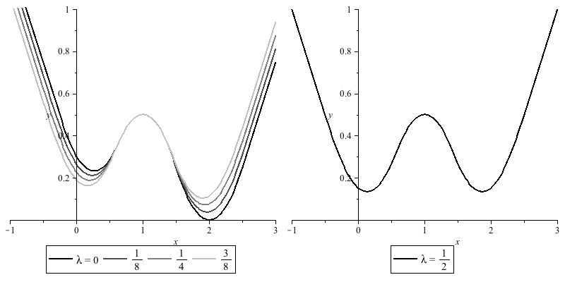
Considering the specific example r=2r=2, and applying ϵ=12\epsilon=\frac{1}{2}, we define the function G⁡(x¯,λ):=(λ​e2​g0+(1−λ)​e2​g1)​(x¯),G(\bar{x},\lambda):=(\lambda e_{2}g_{0}+(1-\lambda)e_{2}g_{1})(\bar{x}), which can be expanded to

G⁡(x¯,λ)={−x¯−λ2+14,x<−12λ​x¯2+(λ−1)​x¯−λ−14,x∈[−12,3−2​32)x¯2+(λ−1)​(4−2​3)​x¯−(λ−1)​(11−6​3)2,x∈[3−2​32,12](1−2​λ)​x¯2+[−4+2​3+(6−2​3)​λ]​x¯+11−6​32−(6−3​3)​λ,x∈(12,3−32]−x¯2+2​x¯−12,x∈(3−32,1+32)(2​λ−1)​x¯2+[2−(2+2​3)​λ]​x¯−12+(2+3)​λ,x∈[1+32,32)x¯2−[4−(4−2​3)​λ]​x¯+4−5−2​32​λ,x∈[32,1+2​32](1−λ)​x¯2+(5​λ−4)​x¯+4−234​λ,x∈(1+2​32,52]x¯+λ2−94,x<52.G(\bar{x},\lambda)=\begin{cases}-\bar{x}-\frac{\lambda}{2}+\frac{1}{4},&x<-\frac{1}{2}\\ \lambda\bar{x}^{2}+(\lambda-1)\bar{x}-\frac{\lambda-1}{4},&x\in[-\frac{1}{2},\frac{3-2\sqrt{3}}{2})\\ \bar{x}^{2}+(\lambda-1)(4-2\sqrt{3})\bar{x}-\frac{(\lambda-1)(11-6\sqrt{3})}{2},&x\in[\frac{3-2\sqrt{3}}{2},\frac{1}{2}]\\ (1-2\lambda)\bar{x}^{2}+[-4+2\sqrt{3}+(6-2\sqrt{3})\lambda]\bar{x}+\frac{11-6\sqrt{3}}{2}-(6-3\sqrt{3})\lambda,&x\in(\frac{1}{2},\frac{3-\sqrt{3}}{2}]\\ -\bar{x}^{2}+2\bar{x}-\frac{1}{2},&x\in(\frac{3-\sqrt{3}}{2},\frac{1+\sqrt{3}}{2})\\ (2\lambda-1)\bar{x}^{2}+[2-(2+2\sqrt{3})\lambda]\bar{x}-\frac{1}{2}+(2+\sqrt{3})\lambda,&x\in[\frac{1+\sqrt{3}}{2},\frac{3}{2})\\ \bar{x}^{2}-[4-(4-2\sqrt{3})\lambda]\bar{x}+4-\frac{5-2\sqrt{3}}{2}\lambda,&x\in[\frac{3}{2},\frac{1+2\sqrt{3}}{2}]\\ (1-\lambda)\bar{x}^{2}+(5\lambda-4)\bar{x}+4-\frac{23}{4}\lambda,&x\in(\frac{1+2\sqrt{3}}{2},\frac{5}{2}]\\ \bar{x}+\frac{\lambda}{2}-\frac{9}{4},&x<\frac{5}{2}.\end{cases}

By Lemma 5.1, we know that

argminx¯P​Ar​(x¯,λ)=argminx¯G​(x¯,λ).\operatornamewithlimits{argmin}\limits_{\bar{x}}PA_{r}(\bar{x},\lambda)=\operatornamewithlimits{argmin}\limits_{\bar{x}}G(\bar{x},\lambda).

Figure 2 displays graphs of GG for various values of λ.\lambda.

Refer to caption
Figure 2: G⁡(x¯,λ)G(\bar{x},\lambda)

Noting that G∈𝒞1,G\in\mathcal{C}^{1}, we find three critical points (where ∂∂x​G​(x,λ)=0\frac{\partial}{\partial x}G(x,\lambda)=0):

  1. 1.

    x¯1=(1−λ)​(2−3)\bar{x}_{1}=(1-\lambda)(2-\sqrt{3}) (leftmost local minimum argument),

  2. 2.

    x¯2=1\bar{x}_{2}=1 (local maximum argument),

  3. 3.

    x¯3=2−(2−3)​λ\bar{x}_{3}=2-(2-\sqrt{3})\lambda (rightmost local minimum argument).

Observe that when λ=12\lambda=\frac{1}{2} we have that x¯1=2−32\bar{x}_{1}=\frac{2-\sqrt{3}}{2}, x¯3=2+32,\bar{x}_{3}=\frac{2+\sqrt{3}}{2}, and

G⁡(2−32,12)=2−32=G⁡(2+32,12).G(\frac{2-\sqrt{3}}{2},\frac{1}{2})=\frac{2-\sqrt{3}}{2}=G(\frac{2+\sqrt{3}}{2},\frac{1}{2}).

This verifies that there are two minimizers when λ=12.\lambda=\frac{1}{2}. Finally, we note that

G⁡(x¯1,λ)<G⁡(x¯3,λ),λ∈[0,12)\displaystyle G(\bar{x}_{1},\lambda)<G(\bar{x}_{3},\lambda),\penalty\ \lambda\in[0,\frac{1}{2}) and G⁡(x¯1,λ)>G⁡(x¯3,λ),λ∈(12,1],\displaystyle G(\bar{x}_{1},\lambda)>G(\bar{x}_{3},\lambda),\penalty\ \lambda\in(\frac{1}{2},1],

which proves the argmin is a singleton whenever λ≠12.\lambda\neq\frac{1}{2}. Therefore, argminPAr\operatornamewithlimits{argmin}PA_{r} is not a continuous function of λ.\lambda.

6 Conclusion

We have seen that, using the Moreau envelope definition, the NC-proximal average can be generalized to accomodate any finite number of suitable functions. Under appropriate conditions, P​ArPA_{r} is well-defined, lower-𝒞2,\mathcal{C}^{2}, and locally Lipschitz continuous in xx and in λ.\lambda. These properties make P​ArPA_{r} a useful function for researchers in the Optimization field.

References

  • [1] H. Bauschke, R. Goebel, Y. Lucet, and X. Wang. The proximal average: basic theory. SIAM J. Optim., 19(2):766–785, 2008.
  • [2] H. Bauschke, Y. Lucet, and M. Trienis. How to transform one convex function continuously into another. SIAM Rev., 50(1):115–132, 2008.
  • [3] H. Bauschke, Y. Lucet, and X. Wang. Primal-dual symmetric intrinsic methods for finding antiderivatives of cyclically monotone operators. SIAM J. Control Optim., 46(6):2031–2051, 2007.
  • [4] H. Bauschke, S. Moffat, and X. Wang. The resolvent average for positive semidefinite matrices. Linear Algebra Appl., 432(7):1757–1771, 2010.
  • [5] H. Bauschke and X. Wang. The kernel average for two convex functions and its application to the extension and representation of monotone operators. Trans. Amer. Math. Soc., 361(11):5947–5965, 2009.
  • [6] H. Bauschke and X. Wang. Compositions and averages of two resolvents: relative geometry of fixed points sets and a partial answer to a question by C. Byrne. Nonlinear Anal., 74(13):4550–4572, 2011.
  • [7] H. Bauschke, X. Wang, and L. Yao. Autoconjugate representers for linear monotone operators. Math. Program., 123(1, Ser. B):5–24, 2010.
  • [8] B. Gardiner and Y. Lucet. Convex hull algorithms for piecewise linear-quadratic functions in computational convex analysis. Set-Valued Var. Anal., 18(3-4):467–482, 2010.
  • [9] R. Goebel. The proximal average for saddle functions and its symmetry properties with respect to partial and saddle conjugacy. J. Nonlinear Convex Anal., 11(1):1–11, 2010.
  • [10] R. Goebel, W. Hare, and X. Wang. The optimal value and optimal solutions of the proximal average of convex functions. Nonlinear Anal., 75(3):1290–1304, 2012.
  • [11] W. Hare. A proximal average for nonconvex functions: a proximal stability perspective. SIAM J. Optim., 20(2):650–666, 2009.
  • [12] W. Hare and C. Planiden. Parametrically prox-regular functions. Journal of Convex Analysis, 21(4), 2014.
  • [13] W. Hare and R. Poliquin. Prox-regularity and stability of the proximal mapping. J. Convex Anal., 14(3):589–606, 2007.
  • [14] J. Johnstone, V. Koch, and Y. Lucet. Convexity of the proximal average. J. Optim. Theory Appl., 148(1):107–124, 2011.
  • [15] S. Kum. Resolvent average on second-order cone. Taiwanese J. Math., 15(6):2733–2750, 2011.
  • [16] Y. Lucet. What shape is your conjugate? A survey of computational convex analysis and its applications [reprint of mr2496900]. SIAM Rev., 52(3):505–542, 2010.
  • [17] R. Rockafellar and R. Wets. Variational analysis. Grundlehren der Mathematischen Wissenschaften [Fundamental Principles of Mathematical Sciences]. Springer-Verlag, Berlin, 1998.
  • [18] X. Wang. Self-dual regularization of monotone operators via the resolvent average. SIAM J. Optim., 21(2):438–462, 2011.