Scale-dependent dipolar modulation and the quadrupole-octopole alignment in the CMB temperature
Abstract
The connection between the dipolar modulation asymmetry and the quadrupole-octopole alignment in the CMB is studied in this work. First, a generalization of the dipolar modulation model is proposed by considering that the amplitude may depend on the scale. As derived from a Bayesian inference analysis, this model fits the CMB data better than the scale-independent one. As an extension of the standard model, the scale-dependent dipolar modulation shows comparable evidence to the standard isotropic model in the large scales (). The posterior distribution of the parameters of the scale-dependent model suggests that the amplitude of the dipolar modulation is large at the lowest multipoles. This large asymmetry induces a detectable correlation between the quadrupole and the octopole. The significance of the quadrupole-octopole alignment is analyzed under the assumption that the Universe has a scale-dependent dipolar modulation. The three alignment estimators considered in this paper show an increment of in the p-value, showing a clear correlation between these two CMB anomalies. Within this new scenario, only one of the alignment estimators is still below the probability level.
1 Introduction
The standard cosmological model provides a good fit to the recent precise observations of the temperature and polarization of the Cosmic Microwave Background (CMB) radiation [1]. However, there exists some slight deviations in the temperature field at the largest scales which might indicate that new physics is needed in order to have a full description of the Universe. Several anomalies have been reported in the literature, many of them reflecting that the large-scale CMB anisotropies do not follow the statistical isotropy expected in the standard model. In particular, CMB data reflects that there is an hemisphere of the sky which has more power than the opposite one [2, 3, 4, 5, 6, 7]. Different estimators have been proposed to characterize this anomaly. In particular, the dipolar modulation model allow us to determine what is the preferred direction on the sky and the degree of asymmetry observed in the CMB temperature [8]. It is plausible that some of these deviations are not independent (see [9] for an analysis of the correlation among the most common large-scale isotropy estimators within the standard model).
Another well-known large-scale anomaly is the alignment between the quadrupole and the octopole [10, 11]. This alignment clearly indicates the existence of a preferred direction in the CMB temperature. Indeed, the alignment of the lowest multipoles could be responsible for the large-scale structures observed in the Ecliptic southern hemisphere [12, 13]. The coincidence that these structures are located in the same region of the sky where the variance asymmetry is observed suggests an eventual relation between the dipolar modulation and the quadrupole-octopole alignment. This possible correlation between the alignment and the (scale-invariant) dipolar modulation has been already studied in [14, 8]. It was found a negligible connection between both anomalies in this case. In this work, we propose to generalize the standard dipolar modulation model by including a scale dependence in the amplitude. Evidences that the dipolar modulation may depend on the scale have been already observed in [6] by computing the modulation on different multipole intervals. In particular, the amplitude of the modulation at the largest scales seems to be greater than the ones derived from smaller scales. This may cause that the effective modulations of the quadrupole and octopole moments are larger than expected from the standard scale-invariant model, and hence, a non-negligible effect on the quadrupole-octopole alignment may be observed.
This paper is organized as follows: the scale-dependent dipolar modulation model is introduced in section 2 as a generalization of the scale-invariant one. The inpainting procedure used in the analysis of the CMB temperature is described in section 3, whereas the iterative posterior estimation method for these maps and the details of the likelihood calculation are shown in sections 4 and 5. The results on the scale-dependent dipolar modulation model are presented in section 6. Finally, the quadrupole-octopole alignment estimators and the corresponding results derived from them for the scale-dependent dipolar modulation model are shown in sections 7 and 8, respectively. The overall conclusions of the paper are presented in section 9.
2 Dipolar modulation model
A non-isotropic model of the CMB temperature based on the modulation of an isotropic field has been proposed to reproduce the hemispherical asymmetry observed in the CMB [14, 8]. If the dipolar model is tested at different scales, then a clear dependence with the multipole is observed [6]. In this section, we introduce the scale-dependent dipolar modulation model by generalizing the scale-independent one previously considered in the literature.
2.1 Scale-independent modulation
In general, anisotropic models of the CMB temperature can be obtained by multiplying an isotropic field by a modulating function:
| (2.1) |
where can be expanded in terms of the spherical harmonics:
| (2.2) |
In the case of the dipolar modulation, we assume that the modulating function only has contributions from the monopole () and the dipole (). Therefore, it is considered that
| (2.3) |
where is a three-dimensional vector parameterizing the dipolar modulation. Notice that the monopole () is chosen such that the isotropic model is recovered when . Extensions of this model could include a monopole term in order to account for an isotropic low variance.
2.2 Scale-dependent modulation
It is possible to generalize the modulation by considering a scale dependence in the model. First, we decompose the isotropic CMB temperature field in the different multipole moments:
| (2.4) |
where the field represents the -th multipolar moment of the field. These moments can be expanded in terms of the spherical harmonics:
| (2.5) |
In this work, we consider a generalization of the model presented in eq. (2.1) in the following way:
| (2.6) |
where the modulating function depends on the multipole. In particular, we have the following expression for the scale-dependent dipolar modulation:
| (2.7) |
In general, the parameter space of this model is given by the components of the vectors . In order to simplify the model and reduce the number of parameters, we consider the following parametric expression for these vectors:
| (2.8) |
We have assumed that the direction of the dipolar modulation is the same for all the scales, which is given by the amplitude vector . However, the amplitude depends on multipole following a power-law with tilt . This model of scale-dependent dipolar-modulation has four parameters: the three components of the vector , which characterizes the direction and the amplitude of the modulation at the pivot multipole , and the parameter representing the scale dependence. The pivot multipole can be freely chosen, since it is not a parameter of the model (we can change the pivot multipole by redefining the amplitude of the vector ). However, it is possible to reduce the correlation between and by considering a suitable pivot scale. For this reason, we use the value for the pivot multipole in our analysis. Finally, notice that the scale-independent model is recovered when .
It is possible to write the scale-dependent model given by eqs. (2.6) and (2.7) as a convolution is real space:
| (2.9) |
where the function is given by the filter coefficients .
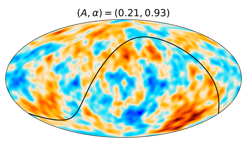
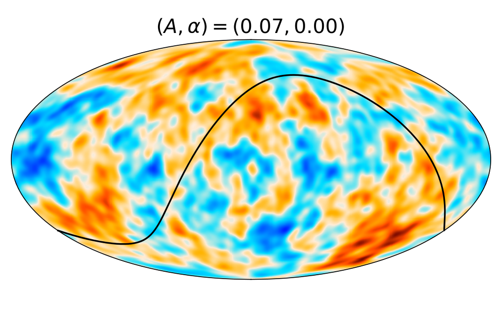
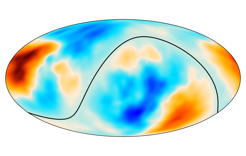
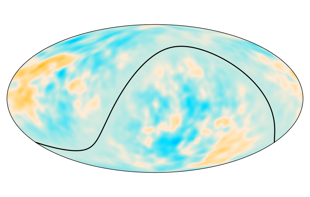
In figure 1, it is shown a simulation of the dipolar modulation considering both the scale-dependent and the scale-invariant models described above. The amplitude of the scale-invariant model is given in [8], and the parameters of the scale-dependent model are chosen to be similar to the ones derived in this work. The effect of the dipolar modulation on the lower multipoles is enhanced in the scale-dependent model with respect to the case of the standard dipolar modulation with constant amplitude. In particular, this may imply a larger correlation between the low multipoles.

3 Inpainting with constrained realizations
Since the CMB temperature maps may have foregrounds residuals, a confidence mask is provided by the component separation methods covering mainly the galactic plane and other regions with high foreground contamination. The incomplete sky makes that spherical harmonic analyses are complicated due to multipole correlations and the presence of a bias in the angular power spectrum estimation. However, this methodological difficulties can be overcome if the mask region is filled with inpainted data.
Assuming that we have a probabilistic model for our sample, the inpainting can be done coherently with this model and the available data outside the mask. The procedure of inpainting with constrained realizations relies on the calculation of the conditional probability density , where is a vector representing the inpainted field and corresponds to the data we are able to observe. Under the hypothesis that the field is Gaussian, we only need the pixel covariance matrix, which can be calculated from the angular power spectrum :
| (3.1) |
where is the unit vector representing the th-pixel. The maximum multipole included in the sum is considered large enough to ensure that the covariance matrix is not singular and positive definite. In our analysis, the value is used for maps with . Since the matrix has dimension , we are limited to low resolution maps due to numerical capabilities.
The procedure we follow to calculate the constrained realizations does not need any matrix inversion. The first step consists in reordering the columns and rows of such that all the observed pixels are in the first entries and the masked pixels in the last indices. Once we have this particular order in the new matrix , its Cholesky decomposition is calculated:
| (3.2) |
where is a lower triangular matrix, which has the following representation in blocks:
| (3.3) |
Whilst and in this expression are both lower triangular matrices, is a rectangular matrix with dimensions the number of masked pixels by the number of observed pixels.
The Cholesky decomposition allow us to calculate Gaussian realizations of the field by calculating the product
| (3.4) |
where and are Gaussian random numbers with zero mean and unit variance. Since we are interested in generating the field given the data , the following system of equations has to be solved
| (3.5) |
| (3.6) |
The first linear equation can be solve by recursive substitution to obtain the vector . This solution is denoted by , although we do not need to perform the matrix inversion explicitly in the numerical implementation. Finally, the inpainted data is given by
| (3.7) |
From this expression, it is possible to deduce that is Gaussian random field with the following mean and covariance:
| (3.8) |
| (3.9) |
Notice that the values of the observed pixels only affects to the mean of , not to its covariance. However, the particular geometry of the mask and the theoretical model used to reconstruct the masked pixels have an influence in both the mean and the covariance of .
4 Iterative posterior estimation
In this section, we introduce a novel method to estimate the posterior distributions which are given by inpainted data. Sometimes, it is difficult to calculate the likelihood function for incomplete data when the procedure involves convolutions or Fourier transforms. The simulation of inpainted data is useful to avoid this problems. However, it is important to take into account that fictitious data are included in the analysis. Moreover, the inpainted region could bias the results because they are generated according to a given fiducial model, which may be different to the one preferred by the available data. In the case of parameter estimation, the information of the inpainted data can be removed from the posterior distribution by applying the iterative method explained below.
The posterior distribution of the model parameters is given by
| (4.1) |
where and are the available data and inpainted data, respectively. In this equation, represents the prior distribution, the likelihood function and the evidence of the model. We can calculate the posterior distribution of the parameters given only the observed data by averaging the posterior over the vector:
| (4.2) |
where is the probability of given the data . In practice, the probability distribution cannot be calculated because we do not know the underlying model:
| (4.3) |
The probability density is the one used to calculate the constrained realizations, which in our case is a Gaussian distribution with mean and variance given in eqs. (3.8) and (3.9), respectively. However, we need the posterior density to calculate this integral. For this reason, an iterative method is proposed to find the posterior. This method is based on the calculation of a sequence of posterior densities such that they converge to the real posterior . The recursive equations are given by the expressions in eqs. (4.2) and (4.3). The -th posterior is calculated from the following integral
| (4.4) |
where depends on the posterior in the previous step:
| (4.5) |
We summarize the iterative procedure in the following steps, assuming that a Markov Chain Monte Carlo (MCMC) method is used for the sampling:
- 1.
We choose a initial posterior , which must be close to the real posterior in order to have a fast convergence. The initial guess can be a Dirac delta at the fiducial model , typically the best-fit CDM model.
- 2.
We simulate a set of constrained realizations by using the probability , which depends on the observed data and the parameters of the model. In this case, the set of parameters assumed in each constrained realization are sampled with the distribution . For instance, the parameters are fixed to the fiducial model in all the constrained realizations in our initial guess (). At the end of this step, we have a set of inpainted data (), where the probability distribution of the vectors is . Notice that we do not need to calculate the integral in eq. (4.5) explicitly in our methodology. Only samples of inpainted data following the conditional distribution are needed.
- 3.
We estimate the posterior for each data set (typically by running a MCMC sampler), obtaining the set of posteriors .
- 4.
The posteriors are averaged in order to obtain the next posterior in the iteration procedure:
(4.6) The result of this expression is a Monte Carlo estimate of the integral in eq. (4.4). If the sampling method is based on a MCMC algorithm, we can calculate posterior samples directly from the Markov chains. Once the burn-in points are removed from the chains, a single set of samples of the parameter space is obtained for each posterior by combining all the samples of the chains generated by the MCMC algorithm. Finally, the union of all the samples of the posteriors () characterizes the distribution of the posterior 11 1 Here we have assumed that the number of samples of each posterior are the same. If not, we have to weight the samples in order to assure that all the posteriors contribute equally to the mean posterior ..
- 5.
The posterior obtained in the previous step is used in step 2 (as the posterior ) to generate the new set of inpainted data for the next iteration. Notice that the set of parameters needed to calculated the constrained realizations in the step 2 can be obtained directly by taking random samples of the posterior as calculated in the step 4.
5 Likelihood
Since we analyze full-sky constrained realizations in the iterative method explained above, the likelihood in harmonic space is simpler than in the case of masked data due to the lack of correlations between different multipoles. In order to calculate the likelihood, the first step is to relate the harmonic coefficients of the modulated field with the ones characterizing the isotropic field . These equations have been obtained for the scale-independent case in previous analysis of the dipolar modulation [15]. Here we generalize that expressions for the scale-dependent dipolar modulation (see appendix A):
| (5.1) |
where is the modulus of the vector and the coefficients are given by
| (5.2) |
In order to obtain these equations, we have assumed the dipolar modulation directions are the same for all the multipoles (the vectors are parallel) and that direction is aligned with the positive axis. By choosing this particular system of reference on the sphere, the coefficients with different ’s are not couple in eq. (5.1), which simplifies its inversion. For a given , eq. (5.1) corresponds to a system of linear equations whose matrix is tridiagonal. The solution of this system can be obtained very fast by using a simplified version of the Gaussian elimination algorithm (see appendix B). During this process of inversion, the Jacobian of the transformation can also be calculated as a byproduct.
Given a scale-dependent dipolar modulation model , the likelihood function is calculated as follows:
- 1.
The spherical harmonics transform of the full-sky data is calculated. Notice that this calculation does not depend on the parameters of the model , and therefore, it can be done only one time at the beginning of the posterior sampling.
- 2.
The spherical harmonics coefficients calculated in the previous step are rotated according to the dipolar modulation direction given by the unit vector , so that the direction of asymmetry corresponds to the axis. The resulting coefficients are the that appear in eq. (5.1).
- 3.
- 4.
Finally, the likelihood function in terms of the coefficients is given by the Gaussian probability density:
(5.3) where the Jacobian is included due to the change of variables done before, from to . The coefficients in this equation represent the smoothing filters present in our data (typically resolution beam and pixel window function).
6 Results on the scale-dependent dipolar modulation model
In this section, the results on the scale-dependent dipolar modulation are given and discussed. In the following subsections, we present the parameter distribution obtained in the sampling of the posterior, and the Bayesian inference analysis comparing the scale-dependent model with the scale-invariant one and the standard model. In addition, a CMB temperature field without the dipolar modulation is estimated from the data and the dipolar modulation parameters. A map of the dipolar modulation anomaly is also given at the end of this section.
The CMB data used in the analysis are the temperature maps provided by the Planck collaboration [1, 16]. We perform the inpainting on maps as described in section 3 at the Healpix resolution . The temperature field is smoothed with both a Gaussian filter whose FWHM is and the corresponding pixel window function of the resolution. The maximum multipole considered in the likelihood is . We have verified that the procedure with these specifications does not have any measurable systematic effect due to the pixelization, inpainting or any other approximate numerical calculation. In addition, we have compared the results obtained from two different component separation methods (SEVEM and SMICA) [16] up to the first iteration in the posterior estimation method described in section 4. Similar posterior distributions of the dipolar modulation parameters are recovered from the two data sets.
6.1 Parameter estimation
As explained in the previous sections, the iterative posterior estimation is applied to inpainted CMB data. The sampling of the posterior is done by an affine-invariant Markov Chain Monte Carlo method [17, 18]. These numerical computations provide a sample of the posterior once the burn-in period is removed. The sampled parameters are the three Cartesian components of the amplitude vector at the pivot scale and the index (four parameters in total). Once chains for these parameters are obtained, we can apply the appropriate transformation in order to infer samples of the amplitude (the modulus of ) and dipolar modulation direction .
The methodology used for the parameter estimation has been tested with a simulated temperature field with scale-dependent dipolar modulation. All the steps, including the inpainting, have been done for this simulation. There is not observed bias or systematic effect on the recovered parameters. Similar posterior than the one obtained from the real data is obtained for this simulated temperature map.
The prior for the dipolar modulation parameters assumed in the sampling is given by the natural limitations of the model. In order to have a positive define covariance matrix, the amplitude of the dipolar modulation must be less than one for all the multipoles. Otherwise, the modulating function in eq. (2.1) vanishes for some directions resulting in a singular covariance matrix for the modulated temperature . Moreover, the dipolar modulation model with an amplitude greater than one does not reproduce the hemispherical variance asymmetry observed in the CMB. Indeed, the modulated field has a ring of zero variance instead of the dipolar asymmetry in this case. The other restriction refers to the index . In this case, we only consider models for which the dipolar modulation decreases with the multipole, that is, is restricted to be non-negative. Otherwise, the amplitude would be greater than one for large enough multipoles, resulting again in a singularity in the covariance matrix and the wrong physical behaviour as in the previous case. The prior distribution is considered to be uniform within the intervals described above. These constraints on the parameters of the model define a improper prior (it is not possible to normalize the prior to unity because there is no an upper bound in ). This is not a problem for the sampling because we only need the unnormalized posterior in this case. However, improper priors can be an issue when different models are compared through the Bayes factor. In this case, we need to get samples of a (proper) prior in order to calculate the evidence (see below the discussion on the Bayes factor).
Since the dipolar modulation is given by a three-dimensional vector, directional statistics must be applied to the sampled distributions. This statistics is preferred to study the dipolar modulation because the significance of the detection can be derived directly from the deviation of the zero vector. The mean amplitude vector is defined as the average of the samples of , that is,
| (6.1) |
where the samples , with , are obtained from the Markov chains. Notice that this average is directly calculated from the vectors, not the amplitudes, in order to take into account the directional character of the dipolar modulation. The mean amplitude vector is in the case of the isotropic standard model. However, this is not the case of the mean of the modulus (not averaged as vectors), which is different from zero even for the standard model. For this reason, the vector statistics is used to quantify the dipolar modulation anomaly. Following this idea, the variance of is defined to be:
| (6.2) |
where the square means the dot product of vectors.
The directional statistics of the dipolar modulation vector at the pivot multipole are given in table 1. In this case, the distribution is marginalized over the index . By comparing the modulus of the vector and its standard deviation, it is obtained that the dipolar modulation is detected with a significance of .
| Vector statistics | ||||
| 0.209 | 0.083 | |||
In figure 2, the marginalized distributions of the dipolar modulation parameters are shown. As in the case of the scale-invariant dipolar modulation, the amplitude is clearly different from zero indicating the existence of an anisotropic pattern in the sky. On the other hand, the distribution of the index shows that a dipolar modulation with a scale dependence is more likely than the scale-invariant case. In particular, the value of is larger than with a probability of . The different statistics of the model parameters shown in figure 2 are given in table 2.
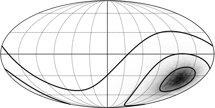
| Posterior statistics | ||||||||||
| Mean | Std. | Percentiles | Best fit | |||||||
| 0.5% | 2.5% | 16% | 50% | 84% | 97.5% | 99.5% | ||||
| A | 0.240 | 0.082 | 0.049 | 0.081 | 0.153 | 0.241 | 0.326 | 0.393 | 0.425 | 0.172 |
| 0.93 | 0.35 | 0.13 | 0.31 | 0.62 | 0.89 | 1.21 | 1.77 | 2.33 | 0.59 | |
| Mean | Contours | Best fit | ||||||||
| 39% | 86% | 99% | ||||||||
6.2 Bayesian inference analysis
Finally, the scale-dependent dipolar modulation model is compared with the scale-invariant case () previously assumed in the literature [14, 8]. Additionally, the two dipolar modulation models are contrasted with the standard isotropic model. This comparison is done in terms of the Bayesian evidence, which is given by the mean of the likelihood function over the prior distribution:
| (6.3) |
where represents the inpainted data. In order to calculate the evidence we generate several full-sky simulations following the probability , where are the parameters of some fiducial model (no dipolar modulation in our case). The likelihood can be easily computed for these full-sky realizations and the above integral can be calculated by Monte Carlo integration (the likelihood function is averaged over samples of the prior distribution). The marginalized evidence can be calculated by the importance sampling method:
| (6.4) |
where the sum is over different inpainted realizations. Notice that the evidence does not depend on the fiducial model used for generating the inpainted realizations. The information of is average out in the above integration.
Since we have to generate prior samples for estimating the evidence, the prior distribution must be normalized to unity. The normalization is also important because the evidence given in eq. (6.3) depends on this normalization factor. The improper prior probability density considered previously can be normalized just by considering a maximum allowed index . In principle, there is not a concrete value for the maximum index which can be said to be natural, although large values of give extremely steep models. We assumed that in the calculation of the evidence. Since the likelihood vanishes for values greater than this index, the evidence for larger values of can be estimated by considering the ratio of indices.22 2 Assuming that the likelihood vanishes for , the evidence calculated with a uniform prior in the range transforms as (6.5) with .
The Bayes factor is defined as the ratio of evidences of two different models. If , the model in the numerator is favoured with respect to the one in the denominator. Depending on the value of the preference of a model against the other is more or less significant. According to the standard criteria, the Bayes factor starts to be significant when and it is clearly decisive when [19].
The Bayes factors of the scale-dependent and scale-invariant dipolar modulation models with respect to the standard isotropic model are shown in table 3. The dipolar modulation with is strongly disfavoured with respect to the standard model in terms of the Bayesian evidence. This is a reflection of the fact that the standard model offers a good overall fit to the CMB temperature data. In principle, it is difficult to find an extension of the standard model with greater evidence, since the observed large-scale deviations are dominated by the cosmic variance and their significance is not high enough to have a large weight in the Bayesian inference. However, the scale-dependent dipolar modulation has an evidence comparable to the one obtained from the standard model. This indicates that the new model of dipolar modulation with scale dependence agrees with the large-scale CMB temperature data () as well as the standard model.
A similar study in terms of the Bayesian evidence of the scale-invariant dipolar modulation has also been done previously in [8]. However, in that paper, it is considered a much smaller prior for the dipolar modulation amplitude (). If we rescale the evidences obtained in that paper in order to have the same prior than the one considered in this work, it is obtained that , which is a strong evidence against the scale-invariant dipolar modulation with respect to the standard model. Although this value is greater than the Bayes factor given in table 3 for the same case (), the two numbers agree on rejecting the scale-invariant model. The remaining difference between these two Bayes factors could be caused by the different dipolar modulation model and resolution considered in [8].33 3 Two additional parameters are considered in the dipolar modulation model in [8]. These parameters modified the isotropic part of the model allowing for additional degrees of freedom in the variation of the angular power spectrum with multipole. In principle, these nuisance parameters may accommodate the observed low variance in the largest scales of the CMB. Notice that the dependence of the prior on the maximum amplitude is strong because it scales with the volume, and therefore, a factor of three must be included in the volume term. We argue that the prior of the amplitude assumed in our analysis () only relies on the validity of the model (the covariance matrix of the modulated field becomes singular for larger values of the amplitude), and not in a value given ad hoc or specified in terms of the posterior distribution.
As discussed above, the evidence of the scale-dependent model depends on the value of assumed in the prior distribution. We can always have an arbitrary small evidence by considering a large enough value of . Therefore, a maximum value of the index must be taken as the limit of the power law model. In order to have a Bayes factor supporting the standard model (), the value of the maximum index should be greater than . In this extreme scenario, the power law model for the dipolar modulation amplitude gives a contribution in the multipoles less than of the corresponding amplitude of the quadrupole. Therefore, this class of models will be better described by a term only modulating the quadrupole, not a power law model as considered in this work. Since with probability , models with such a large value of the index are not favoured by the data (see table 2). In the light of this analysis, we claim that the conclusion that the scale-dependent dipolar modulation has similar evidence than the standard model is quite robust in spite of the ambiguity of the evidence due to the dependence on . Notice that the criteria for model selection in Bayesian inference are given in terms of , and therefore, the dependence of this quantity on is also logarithmic, giving a weak dependence of the results on the maximum index considered.
On the other hand, it is found that when comparing the scale-dependent and the scale-independent scenarios (see table 3). This large Bayes factor strongly supports the dipolar modulation model with scale dependence () against the standard dipolar modulation with scale-invariant amplitude.
| Bayes factor with respect to the SM | Difference | ||
| scale-dependent DM | scale-invariant DM | ||
| -0.057 | -2.18 | 2.13 | |
6.3 CMB temperature without dipolar modulation and the anomaly map
Finally, it is possible to remove statistically the observed dipolar modulation from the data, obtaining a more isotropic temperature field. This map would be an attempt to obtain a CMB temperature field which is more compatible with the isotropic CMB model than the observed data. The procedure for calculating this isotropic map consists in applying the same transformation described in section 5 used for calculating the likelihood. The relation between the spherical harmonics coefficients given in eq. (5.1) has to be inverted in order to calculate the isotropic coefficients from the ones characterizing the field with dipolar modulation (). (see appendix B for the details of the inversion). The dipolar modulation parameters assumed in the inversion are the ones given in table 1, that is, . The resulting maps of this procedure are shown in figure 3. We can see that, once the dipolar modulation is removed, the temperature field seems to be more isotropic. The anomaly map is defined to be the difference between the observed CMB data and the isotropic estimation obtained by removing the dipolar modulation. This map shows clearly a large-scale pattern, indicating that most of the dipolar modulation anomaly affects the low multipoles.


7 Quadrupole and octopole alignment
Several estimators have been proposed to quantify the quadrupole-octopole alignment. Here, we discuss three of them previously used in the literature: one based on the angular momentum dispersion and the other two in the multipole vectors formalism.
7.1 Maximum angular momentum dispersion
One of the first estimators proposed in the literature for quantifying the alignment between the quadrupole and the octopole is based on planes with maximum variance [10]. Considering the unit vector , the angular momentum is projected along the direction given by this vector (). The variance of this quantity measures the amplitude of the fluctuations on planes perpendicular to .44 4 In the particular case when the -direction is given by , it is possible to see that the operator is proportional to the derivative with respect to the azimuthal angle . Therefore, the variance of this quantity measures how much the field varies on the direction perpendicular to . Decomposing the temperature field in the different multipolar moments , the variance of the angular momentum projected on the -direction as a function of is given by
| (7.1) |
where are the spherical harmonic coefficients calculated in the system of reference in which the -axis is parallel to . Given the spherical harmonic coefficients in an arbitrary system of reference, the coefficients can be calculated by applying the appropriate Wigner D-matrix. Finally, the direction characterizing the multipole is calculated by maximizing the angular momentum variance given in eq. (7.1).
Since different multipoles are independent in an isotropic field, the directions given by would also be independent. If this is the case, the cosine of the angle between two directions, , is uniformly distributed in the interval . Notice that the quantity given in eq. (7.1) is invariant under parity transformation , and therefore, the sign of is not relevant. In the present analysis, we quantify the quadrupole-octopole alignment with the estimator , which is uniformly distributed in the range according to the standard model. Values of very close to may imply an unexpected alignment between these two multipoles.
7.2 Multipole vectors
In addition to the standard expansion in terms of the spherical harmonics, there are other ways to represent a field on the sphere. One of them used in isotropy analysis of the CMB is the multipole vectors decomposition [20, 21]. In this formalism, the -component of the temperature field is expressed as a function of unit vectors, , and an amplitude .
| (7.2) |
where removes the contribution of lower order multipoles from the preceding product. Notice that, in the case of the dipole, all the information is given by a vector, , as it is expected from the standard decomposition in terms of the spherical harmonics.55 5 In the case of the dipole, the components of the vector are given by the following expressions in terms of the spherical harmonics coefficients: (7.3a) (7.3b) (7.3c) The multipole vectors approach generalizes this well-known characterization of the dipole to higher-order multipoles.
In this scheme, the isotropy of the field can be tested by estimating the amount of alignment between different multipole vectors. Since there are many vectors for each multipole (two representing the quadrupole, and three for the octopole), several combinations of vectors can be considered. In this work, we use two alignment estimators that have been used previously in the literature [11].
Given two multipole vectors, the area vector is defined by the cross product:
| (7.4) |
In our case, we are only interested in the quadrupole and the octopole, and hence, there is only an area vector for the quadrupole and three vectors for the octopole:
| (7.5a) | |||
| (7.5b) |
Notice that the vector derived from the quadrupole is the same than the one obtained with the maximum angular momentum dispersion ( in the previous section). However, there is no a direct correspondence between the vectors and in the case of the octopole [12].
In general, the alignment of these vectors with an arbitrary direction can be quantified by the dot product. Therefore, the quadrupole-octopole alignment is characterized by the three following quantities:
| (7.6) |
In order to combine all the information, two estimators are proposed [11]:
| (7.7a) | |||
| (7.7b) |
Whereas the estimator represents the average of the alignment vectors, is a quadratic combination of these vectors. Both estimators take values in the range , being the maximum alignment.
8 Results on the quadrupole-octopole alignment
In this work, the implications of the scale-dependent dipolar modulation model on the alignment of the quadrupole and octopole are explored. From eq. (5.1), it can be shown that the dipolar modulation adds correlations between consecutive multipoles, then a quadrupole-octopole correlation is expected. If the amplitude of the dipolar modulation is large enough for the smallest multipoles, then alignment between the quadrupole and the octopole may be explained within this sort of non-isotropic models. In this section, we quantify the impact of the scale-dependent dipolar modulation model proposed in this work on the quadrupole-octopole alignment.
Once the parameters of the dipolar modulation model are sampled according to the posterior, these samples are used as random realizations of a non-isotropic Universe. A CMB temperature field with a dipolar modulation is generated for each set of parameters following eq. (2.9). Hence, we obtain a sample of CMB simulations for the scale-dependent dipolar modulation model compatible with the posterior. Finally, the probability distribution of the quadrupole-octopole alignment estimators are calculated from theses samples.
In figure 4, the probability distributions of the three alignment estimators analyzed in this work are shown. It is possible to see that the alignment between the quadrupole and the octopole is favoured under the hypothesis that there exists a scale-dependent dipolar modulation with respect to the standard isotropic case. This is particularly evident for , where a clear deviation from the uniform distribution is shown. In the three estimators, values close to one are more likely when the CMB temperature has a scale-dependent dipolar modulation. The -values obtained in each case are shown in table 4. It is found that the alignment probability is larger for the dipolar modulation model than for the isotropic case by a factor of . Only the estimator remains below the level, although its -value has also increased by a similar factor than the others. Notice that this statistical dependence of the two anomalies is only observed if the dipolar modulation is considered to be scale-dependent. This correlation is not observed in the scale-invariant case [22].
| -value | ||
|---|---|---|
| Isotropic | scale-dependent DM | |
9 Conclusions
One of the open questions on CMB physics are the nature of the different large-scale deviations from the standard model observed in the data. In this work, we study the influence of the dipolar modulation on the quadrupole-octopole alignment. Previous analysis have shown that there is a negligible correlation between both anomalies [22]. However, the dipolar modulation model considered in those works assumes that the amplitude of the modulation is independent on the scale. Signatures of a scale-dependent modulation have been reported in [6] by studying the dipolar modulation in different multipole intervals. In this paper, we propose a scale-dependent dipolar modulation model which is more consistent with the data and reproduces the observed large-scale temperature fluctuations. We find that the Bayesian evidence supports the scale-dependent model versus the one with scale-invariant amplitude. Additionally, if the scale-dependent dipolar modulation model is compared to the standard model, similar evidences are obtained (Bayes factor ). Therefore, this new model of dipolar modulation represents a good fit to the CMB data at large scales (), at least, as well as the standard model.
Once a suitable dipolar modulation model is adopted, the alignment between the quadrupole and the octopole is analyzed. Three different estimators commonly used in the literature for quantifying the alignment are studied. The corresponding statistical distributions are calculated under the hypothesis that a scale-dependent dipolar modulation may exists. For this purpose, the parameters of the dipolar model are sampled according to the posterior distribution. Since the dipolar model favours that some region of the sky has more large-scale power than the opposite one, the low multipoles of the CMB must be correlated in a particular way. Therefore, the alignment between the large-scale multipoles is more likely in the dipolar modulation scenario than in the standard model. However, this can be only achieve considering the scale-dependent dipolar modulation. This model makes the distributions of the alignment estimators change with respect to the isotropic case so that the quadrupole-octopole alignment is more likely. We find an increment of a factor of () in the p-value in all the estimators considered. However, there is still a deviation whose -value is below in one of the estimators () based on multipole vectors.
Notice that, in this work, we have only considered the possibility that a particular dipolar modulation model could explain the quadrupole-octopole alignment. However, it is possible that a more general model accounts for several of the large-scale CMB anomalies at the same time reducing the joint significance. For the moment, we have shown that a more realistic dipolar modulation including the scale dependence is clearly correlated with the large-scale CMB alignments, and therefore, these two anomalies are not independent. Further work may consists in finding better models for explaining the observed large-scale deviations in the CMB within a more physical frame.
Appendix A Scale-dependent dipolar modulation in spherical harmonics
In order to calculate the likelihood function or to reconstruct the isotropy map from the data, it is useful to work in the spherical harmonics space. In this appendix, we calculate the spherical harmonics transform of the dipolar modulation model with scale-dependent amplitude. Similar calculation was done before for the constant amplitude model in [15]. For simplicity, we restrict our calculation to the case in which the dipolar modulation direction coincides with the -axis. The dipolar model in eq. (2.9) in spherical coordinates is given by:
| (A.1) |
where is the filter whose coefficients are the scale-dependent dipolar amplitudes given by eq. (2.8) for the model considered in this work. In order to calculate the spherical harmonics coefficients of the product of two functions on the sphere, we use the following identity:
| (A.2) |
The spherical harmonics transform of eq. (A.1) can be calculated from the previous integral and taking into account that :
| (A.3) |
where it has been used that the convolution in eq. (A.1) in Fourier space is just given by the product of the filter and the spherical harmonics coefficients . This equation can be simplified using the selection rules of the Wigner 3- symbols. In this case, only the terms with or contributes to the sum. In this case, the Wigner 3- symbols in the expression above are given by the identity
| (A.4) |
Finally, we obtain the spherical harmonics coefficients of the modulated field in terms of the coefficients characterizing the isotropic part
| (A.5) |
where the coefficients are
| (A.6) |
These equations are the same that the ones in eqs. (5.1) and (5.2) and they are the generalization of the expressions in [15] to the case of scale-dependent dipolar modulation.
Appendix B Recursive estimation of the isotropic spherical harmonics coefficients
The inversion of the system of equations in eq. (5.1) can be done by introducing the following variables, which are calculated by recursion on :
| (B.1a) | |||
| (B.1b) |
with and . Likewise, the spherical harmonics of the isotropic field can be calculated from the modulated coefficients by solving two recursive equations. First, the auxiliary coefficients are computed by
| (B.2) |
with the initial condition . Finally, the coefficients are given by
| (B.3) |
which is solved backwards with the initial condition .
Additionally, the Jacobian of the transformations in eq. (5.1) can also be obtained from the variables defined above:
| (B.4) |
Acknowledgments
AMC would like to thank Universidad de Cantabria for a post-doctoral contract. AMC and EMG acknowledge financial support from Agencia Estatal de Investigación (AEI) and Fondo Europeo de Desarrollo Regional (FEDER, UE), projects ref. ESP2017-83921-C2-1-R and AYA2017-90675-REDC.
References
- [1] Planck Collaboration and Y. Akrami et al., Planck 2018 results. I. Overview and the cosmological legacy of Planck, arXiv e-prints (2018) arXiv:1807.06205 [1807.06205].
- [2] H. K. Eriksen, F. K. Hansen, A. J. Banday, K. M. Górski and P. B. Lilje, Asymmetries in the Cosmic Microwave Background Anisotropy Field, ApJ 605 (2004) 14 [astro-ph/0307507].
- [3] F. K. Hansen, A. J. Banday, K. M. Górski, H. K. Eriksen and P. B. Lilje, Power Asymmetry in Cosmic Microwave Background Fluctuations from Full Sky to Sub-Degree Scales: Is the Universe Isotropic?, ApJ 704 (2009) 1448 [0812.3795].
- [4] Y. Akrami, Y. Fantaye, A. Shafieloo, H. K. Eriksen, F. K. Hansen, A. J. Banday et al., Power Asymmetry in WMAP and Planck Temperature Sky Maps as Measured by a Local Variance Estimator, ApJ 784 (2014) L42 [1402.0870].
- [5] Planck Collaboration and P. A. R. Ade et al., Planck 2013 results. XXIII. Isotropy and statistics of the CMB, A&A 571 (2014) A23 [1303.5083].
- [6] Planck Collaboration and P. A. R. Ade et al., Planck 2015 results. XVI. Isotropy and statistics of the CMB, A&A 594 (2016) A16 [1506.07135].
- [7] Planck Collaboration and Y. Akrami et al., Planck 2018 results. VII. Isotropy and Statistics of the CMB, arXiv e-prints (2019) arXiv:1906.02552 [1906.02552].
- [8] J. Hoftuft, H. K. Eriksen, A. J. Banday, K. M. Górski, F. K. Hansen and P. B. Lilje, Increasing Evidence for Hemispherical Power Asymmetry in the Five-Year WMAP Data, ApJ 699 (2009) 985 [0903.1229].
- [9] J. Muir, S. Adhikari and D. Huterer, Covariance of CMB anomalies, Phys. Rev. D 98 (2018) 023521 [1806.02354].
- [10] A. de Oliveira-Costa, M. Tegmark, M. Zaldarriaga and A. Hamilton, Significance of the largest scale CMB fluctuations in WMAP, Phys. Rev. D 69 (2004) 063516 [astro-ph/0307282].
- [11] C. J. Copi, D. Huterer, D. J. Schwarz and G. D. Starkman, Large-scale alignments from WMAP and Planck, MNRAS 449 (2015) 3458 [1311.4562].
- [12] C. J. Copi, D. Huterer, D. J. Schwarz and G. D. Starkman, On the large-angle anomalies of the microwave sky, MNRAS 367 (2006) 79 [astro-ph/0508047].
- [13] A. Marcos-Caballero, E. Martínez-González and P. Vielva, Local properties of the large-scale peaks of the CMB temperature, Journal of Cosmology and Astro-Particle Physics 2017 (2017) 023 [1701.08552].
- [14] C. Gordon, Broken Isotropy from a Linear Modulation of the Primordial Perturbations, ApJ 656 (2007) 636 [astro-ph/0607423].
- [15] A. Moss, D. Scott, J. P. Zibin and R. Battye, Tilted physics: A cosmologically dipole-modulated sky, Phys. Rev. D 84 (2011) 023014 [1011.2990].
- [16] Planck Collaboration and Y. Akrami et al., Planck 2018 results. IV. Diffuse component separation, arXiv e-prints (2018) arXiv:1807.06208 [1807.06208].
- [17] J. Goodman and J. Weare, Ensemble samplers with affine invariance, Communications in Applied Mathematics and Computational Science, Vol. 5, No. 1, p. 65-80, 2010 5 (2010) 65.
- [18] D. Foreman-Mackey, D. W. Hogg, D. Lang and J. Goodman, emcee: The MCMC Hammer, PASP 125 (2013) 306 [1202.3665].
- [19] H. Jeffreys, Theory of probability. Oxford University Press, Oxford, England, third ed., 1961.
- [20] J. R. Weeks, Maxwell’s Multipole Vectors and the CMB, arXiv e-prints (2004) astro [astro-ph/0412231].
- [21] C. J. Copi, D. Huterer and G. D. Starkman, Multipole vectors: A new representation of the CMB sky and evidence for statistical anisotropy or non-Gaussianity at , Phys. Rev. D 70 (2004) 043515 [astro-ph/0310511].
- [22] L. Polastri, A. Gruppuso and P. Natoli, CMB low multipole alignments in the CDM and dipolar models, Journal of Cosmology and Astro-Particle Physics 2015 (2015) 018 [1503.01611].