On an enhancement of RNA probing data using Information Theory
Abstract
Identifying the secondary structure of an RNA is crucial for understanding its diverse regulatory functions. This paper focuses on how to enhance target identification in a Boltzmann ensemble of structures via chemical probing data. We employ an information-theoretic approach to solve the problem, via considering a variant of the Rényi-Ulam game. Our framework is centered around the ensemble tree, a hierarchical bi-partition of the input ensemble, that is constructed by recursively querying about whether or not a base pair of maximum information entropy is contained in the target. These queries are answered via relating local with global probing data, employing the modularity in RNA secondary structures. We present that leaves of the tree are comprised of sub-samples exhibiting a distinguished structure with high probability. In particular, for a Boltzmann ensemble incorporating probing data, which is well established in the literature, the probability of our framework correctly identifying the target in the leaf is greater than .
Keywords:
RNA structure , chemical probing , Rényi-Ulam game , information theoryMSC
94A15 , 68P30 , 92E10 , 92B051 Introduction
Computational methods for RNA secondary structure prediction have played an important role in unveiling the various regulatory functions of RNA. In the past four decades, these approaches have evolved from predicting a single minimum free energy (MFE) structure (Waterman 1978; Zuker and Sankoff 1984) to Boltzmann sampling an ensemble of possible structures (McCaskill 1990; Ding and Lawrence 2003). Despite its success in a wide range of small RNAs, these thermodynamics-based predictions are by no means perfect.
In parallel, experiments by means of chemical and enzymatic probing have become a frequently used technology to elucidate RNA structure (Stern et al. 1988; Merino et al. 2005; Deigan et al. 2009). These probing methods use chemical reagents to bind unpaired nucleotides and yield reactivities at nucleotide resolution. To some extent, these reactivities provide information concerning single-stranded or double-stranded RNA regions. Recent advances focus on the development of thermodynamics-based computational tools that incorporate such experimental data (Deigan et al. 2009; Washietl et al. 2012; Zarringhalam et al. 2012).
While the use of probing data has significantly improved the prediction accuracy of in silico structure prediction for several classes of RNAs (Lorenz et al. 2011), these methods have not solved the folding problem for large RNA systems, such as long non-coding RNAs (lncRNAs, typically 200–20k bases). The reason is that the footprinting data does not identify base pairing partners of a given nucleotide. In particular, probing data alone cannot distinguish short-range and long-range base pairings. For long RNAs, the existence of the latter, however, has been shown experimentally (Lai et al. 2018) as well as theoretically (Li and Reidys 2018; Li et al. 2019). Thus, even combined with experimental data, there are still numerous RNA folds consistent with the probing data.
We assume that
the ensemble of possible structures is in thermodynamic equilibrium, i.e. a Boltzmann ensemble.
For many classes of RNAs, it is also reasonable to assume that the sequence folds into
a unique structure, the target, which is contained in the ensemble. Hence, the problem of structure prediction gives rise to the following challenge:
| How to enhance target identification in a Boltzmann ensemble of structures? | (1) |
In this paper, we employ an information-theoretic approach in order to solve Problem 1, via considering a variant of the Rényi-Ulam game. Our framework is centered around the ensemble tree, a hierarchical bi-partition of the input ensemble, whose leaves are comprised of sub-samples exhibiting a distinguished structure with high probability. Specifically, the ensemble tree is constructed by recursively querying about whether or not a base pair of maximum information entropy is contained in the target. We prove that the query of maximum entropy base pair splits the ensemble into two even parts and in addition provides maximum reduction in the entropy of the ensemble. These questions can be answered in the affirmative, since the sequence is assumed to a single target. They are answered via relating additional probing data with the initial one, employing the modularity in RNA secondary structures. By this means, we identify the correct path in the ensemble tree from the root to the leaf.
The key result of this paper is that the probability of the ensemble tree correctly identifying the target in the leaf is greater than , for the Boltzmann ensembles incorporating probing data from sequences of length , see Section 4.2. To demonstrate the result, we take into consideration three components. Firstly, we utilize a -Boltzmann sampler with signature distance filtration, which is well suited for Boltzmann ensembles subjected to the probing data constraint (Deigan et al. 2009; Zarringhalam et al. 2012), see Section 2.2. Secondly, we consider the error rates arisen from answering the queries via probing data in Section 3.1. We show that these error rates can be significantly reduced via repeated queries in Section 4.2. Thirdly, we prove that the leaf with low information entropy contains a distinguished structure, see Section 4.1. We present that, once in the correct leaf, the probability the distinguished structure being identical to the target is almost always correct.
To summarize, the key points of our approach are:
- 1.
our method starts with a Boltzmann sample and derives a sub-sample that contains the target with high probability,
- 2.
the derivation is facilitated by means of the ensemble tree, and the identification of the correct path from root to leaf, is obtained by a variant of the Rényi-Ulam game,
- 3.
the answers to the respective queries are inferred from chemical probing, by relating additional probing data to initial one using modularity.
This paper is organized as follows: in Section 2, we introduce the main elements of our framework: the Rényi-Ulam game, the Boltzmann ensemble, base-pair queries and the ensemble tree. In Section 3, we demonstrate how to integrate additional probing data with the initial ones allowing to answer the queries, thereby identifying the correct path. In Section 4, we analyze the ensemble tree and present that our approach identifies the target reliably and efficiently. Finally, we integrate and discuss our results in Section 5.
2 Some background
2.1 The Rényi-Ulam game
We now approach Problem 1 via the Rényi-Ulam game, a two-person game, played by a questioner (Q) and an oracle, (O). Initially O thinks of an integer, , between one and one million and Q’s objective is to identify , asking yes-no questions. O is allowed to lie at a rate specific to yes and no, respectively.
The Rényi-Ulam game has been extensively studied since the early works by Rényi 1961; Ulam 1976, and has various applications such as adaptive error-correcting codes in the context of noisy communication (Shannon 1948; Berlekamp 1968). Depending on the respective application scenario, numerous variants of the Rényi-Ulam game have been considered, specifying the format of admissible queries or the way O lies (Pelc 1989; Spencer 1992).
In what follows, we shall play the following version of the game: O holds a set of bit strings of finite length , not every bit string being equally likely selected and the queries have to following format: “Is the th-bit of the bit string equal to ?”, i.e. Q executes bit query. O’s lies occur at random, are independent and context-dependent. Specifically, O lies with probability and in case of the truthful answer being ”No” and “Yes”, respectively. The particular cases and have been studied in the context of half-lies (Rivest et al. 1980).
The majority of studies on the Rényi-Ulam game to date is combinatorial. That is, they stipulated the number of lies (or half-lies) being a priori known and focused on finding optimal searching strategies which uses a minimum number of queries to identify the target in all cases (Rivest et al. 1980; Spencer 1992).
Within the framework of this paper, we study two distinctly different manifestations of the oracle. The first is embodied as an indicator random variable, whose distribution is derived from a modularity analysis on RNA MFE-structures, see Section 3.1, and the second recruits experimental data, see Section 3.2. In both manifestations, erroneous responses arise intrinsically at random: either as a result of the distribution of the r.v. or intrinsic errors of experimental data.
By construction, this rules out a unique winning strategy for Q: instead, we consider the average fidelity or accuracy to identify the target utilizing a sub-optimal number of queries. We shall propose an entropy-based strategy: at any point a query is selected relative to the subset of bit strings coinciding with the target in all previously identified positions, that maximizes the uncertainty reduction on the subset, see Section 2.4.
2.2 The Boltzmann ensemble
At a given point in time, an RNA sequence, , assumes a fixed secondary structure, by establishing base pairings. Over time, however, assumes a plethora of RNA secondary structures appearing at specific rates, see A for details and context on RNA. These exist in an equilibrium ensemble expressed by the partition function (McCaskill 1990) of .
More formally, the structure ensemble, of is a discrete probability space over the set of all secondary structures, equipped with the probability of folding into . We shall assume that the ensemble of structures is in thermodynamic equilibrium, the distribution of these structures being described as a Boltzmann distribution. The Boltzmann probability, , of the structure is a function of the free energy of the sequence folding into , computed via the Turner energy model (Mathews et al. 1999; Mathews et al. 2004), see B for details. The Boltzmann probability is expressed as the Boltzmann factor , normalized by the partition function, , i.e.
where denotes the universal gas constant and is the absolute temperature. The Boltzmann distribution facilitates the computation of the partition function for each substructure. The partition function algorithm (McCaskill 1990) for secondary structures computes and, in particular, the base pairing probabilities based on the free energies for each structure within the structure ensemble .
Let denote the probability of a base pairing between nucleotides and in the ensemble . Clearly, can be computed as the sum of probabilities of all secondary structures that contain , that is,
where denotes the occurrence of the base pair in .
The thermodynamics-based partition function has been extended to incorporate chemical probing data to generate a Boltzmann ensemble, . These approaches (Deigan et al. 2009; Washietl et al. 2012; Zarringhalam et al. 2012) transform structure probing data into a pseudo energy term, , which reflects how well the structure agrees with the probing data. The Turner free energy is then evaluated by adding the pseudo energy term to the loop-based energy, i.e., . The corresponding equilibrium ensemble, , is distorted in favor of structures that are consistent with probing data, see C.
In D, we utilize the - signature, which is suited for probing data, and quantify the discrepancy between the Boltzmann ensemble and the target via the signature distance . We present that the average distance for an unrestricted ensemble is , while the distance for an ensemble incorporating probing data is reduced to . This motivates us to define a -Boltzmann ensemble, , which consists of structures having signature distance to the target at most , i.e., . In particular, we present that the ensemble has an average normalized signature distance similar to a -ensemble having . In this paper we discuss unrestricted and restricted Boltzmann ensembles, and .
We shall employ greyscale diagrams in order to visualize a sample of secondary structures by superimposing them in one diagram, visualizing the base pairing probabilities. A greyscale diagram displays each base pair as an arc with greyscale , where greyscale represents black and represents white, see Fig. 1.

Instead of computing the entire ensemble, we shall consider sub-samples consisting of secondary structures with multiplicities of and refer to as the sample. For sufficiently large (typically of around size , see Ding and Lawrence 2003), provides a good approximation of the Boltzmann ensemble .
A sample is a multiset of cardinality and for each structure in , its multiplicity, , counts the frequency of appearing in . Thus in the context of , is given by the -multiplicity divided by , . The base pairing probability has its -analogue , where denotes the frequency of the base pair appearing in . We shall develop our framework in the context of the structure ensemble , and only reference the sample , in case the results are particular to .
2.3 The bit queries
Any structure over nucleotides is considered as a bit string of dimension , stipulating (1) a structure is completely determined by the set of base pairs it contains and (2) any position can pair with any other position, except of itself.
The bit query now determines a single bit, i.e. whether or not the base pair is present in the target, stipulating that a unique target is assumed by the sequence in question. The target is also assumed to have the Boltzmann probability as it appears in the ensemble. We therefore associate the query about the target with a random variable, , defined on the ensemble, via questioning the presence of in each structure. By construction, the distribution of is given by the base pairing probability .
Any base pair, , has an entropy, defined by the information entropy of , i.e.
where the units of are in bits. The entropy measures the uncertainty of the base pair in . When a base pair is certain to either exist or not, its entropy is . However, in case is closer to , becomes larger.
The r.v. partitions the space into two disjoint sub-spaces and , where (), and the induced distributions are given by
Intuitively, quantifies the average bits of information we would expect to gain about the ensemble when querying a base pair . This motivates us to consider the maximum entropy base pairs, the base pair having maximum entropy among all base pairs in , i.e.
As we shall prove in Section 4.1, produces maximally balanced splits.
2.4 The ensemble tree
Equipped with the notion of ensemble and bit query (i.e. the respective maximum entropy base pairs), we proceed by describing our strategy to identify the target structure as specified in Problem 1. The first step consists in having a closer look at the space of ensemble reductions.
Each split obtained by partitioning the ensemble using r.v. , can in turn be bipartitioned itself via any of its maximum entropy base pairs. This recursive splitting induces the ensemble tree, , whose vertices are sub-samples and in which its -th layer represents a partition of the original ensemble into blocks. , is a rooted binary tree, in which each branch represents a -induced split of the parent into its two children.
Formally the process halts if either the resulting sub-spaces are all homogeneous, i.e. their structural entropy is , which means that they contain only copies of one structure, or it reaches a predefined maximum level . In our case we set the maximum level to be , that is, the height of the ensemble tree is at most . The procedure is described as follows:
- 1.
start with the ensemble .
- 2.
for each space with , where is a sequence of s and s having length at most , compute:
- (a)
select the maximum entropy base pair of as the feature, i.e.
- (b)
split into sub-spaces and using the feature , that is, for ,
- (a)
- 3.
repeat Step until all new sub-spaces either have structural entropy or reach the maximum level .
In Fig. 2 we display an ensemble tree.

3 Path identification
Given the ensemble tree, we shall construct a path recursively starting from the root to identify the leaf that contains the target. We shall do so by successive bit queries about maximum entropy base pairs, see Fig. 2.
As mentioned before, we employ two manifestations of the oracle, one using modularity based on RNA-folding, see Section 3.1, and the other determining the existence of base pairs by experimental means (Section 3.2).
3.1 The oracle via modularity and RNA folding
Here we shall employ modularity of RNA structures, i.e. the loops, which constitute the additive building blocks for the free energy have only marginal dependencies. This can intuitively be understood by observing that any two loops can only intersect in at most two nucleotides, see B.
Let us introduce the notion of embedding and extraction of a contiguous subsequence or fragment
By construction, we have and a contiguous subsequence or fragment of an RNA sequence is called modular if it being extracted folds into the same arc configuration as it does embedded in the sequence.
Next we show how to employ probing data to reliably answer whether or not a particular (maximum entropy) arc is contained in the target structure. Structural modularity implies that if this arc can indeed be found in the target structure, then a comparative analysis of the probing data of the entire sequence with those of the extracted sequence, as well as the remainder, concatenated at the cut points will exhibit distinctive similarity. Modularity is a decisive discriminant, if, in contrast, random fragments do not exhibit such similarity.
To quantify to what extent modularity can discriminate base pairs, we perform computational experiments on random sequences via splittings. For each sequence, we consider its MFE structure computed via ViennaRNA (Lorenz et al. 2011). Given two positions and , we cut the entire sequence into two fragments, and the remainder , i.e., . Subsequently, the two fragments and refold into their MFE structures and , respectively, which are combined into a structure . If bases and are paired in , such a splitting is referred to as modular and the resulting structure is denoted by . Otherwise, it is called random, with the output structure . We proceed by computing the base-pair and signature distance from the MFE to the structures or . The base-pair distance is one of the most frequently used metrics to quantify the similarity of two different structures viewed as bit strings Zuker 1989; Agius et al. 2010, the signature distance measures the similarity between their signatures, which is well suited within the context of the probing profiles, see A.
Fig. 3 (LHS) compares the distribution of the signature distances and obtained from modular and random splittings, respectively. The structures induced by modular splitting have much more similar probing signatures to their MFE structures, than those induced by random splitting. The situation is analogous for base-pair distances, see Fig. 3 (RHS). Since these distances measure structural similarity, the data also indicates that, when and form a base pair, the fragment is more likely to fold into the same configuration as it does being embedded, i.e. is modular.
 |
 |
The data displayed in Fig. 3 suggests the threshold distance, , for signatures, by which we distinguish modular from random. In order to quantify the accuracy of this classification, we consider the resulting false discovery rate (FDR) and false omission rate (FOR).11 1 where TP (true positive) is the number of correctly identified base pairs, FP (false positive) is the number of incorrectly predicted pairs that do not exist in the accepted structure, TN (true negative) is the number of pairs of bases that are correctly identified as unpaired and FN (false negative) is the number of base pairs in the accepted RNA structure that are incorrectly predicted as unpaired. In our Rényi-Ulam game variation, the expected values of FDR and FOR are the error rates and in case the truthful answer being yes and no, respectively. Fig. 4 displays the error rates and as functions of . For , we compute and , i.e. we have an error rate of for rejecting and an error rate of for confirming a base pair.

3.2 The oracle via experimental data
The identification of base pairs is a fundamental and longstanding problem in RNA biology (Hajdin et al. 2013; Weeks 2015). In E, we summarize state-of-the-art experimental approaches that provide reliable solutions to the problem, and in particular detail two methods, both of which utilize chemical probing (Mustoe et al. 2019; Cheng et al. 2017) and recover duplexes with a false discovery rate less than .
Successive queries recursively split a given ensemble of structures. This induced sequence of splits can be embedded in a binary tree, and be viewed as a path from the root to a leaf. We shall discuss this tree in detail in the next section.
4 The ensemble tree
Given an input sample , we construct the ensemble tree having maximum level , recursively computing the maximum entropy base pairs as described in Algorithm 1. In this section, we shall analyze the entropy of leaves in order to quantify the existence of a distinguished structure and to identify the target.
4.1 Entropy
To quantify the uncertainty of an ensemble, we define the structural entropy of an ensemble, , of an RNA sequence, , as the Shannon entropy
the units of being bits. The sum is taken over all secondary structures of , and denotes the Boltzmann probability of the structure in the ensemble . The notion of structural entropy is originated in thermodynamics and is usually regarded as a measure of disorder, or randomness of an ensemble (Sükösd et al. 2013; Garcia-Martin and Clote 2015).
Given a sample of size , the structural entropy has the upper bound , that is, reaches its maximum when all sampled structures are different. Throughout the paper, we assume and therefore .
Proposition 1
Let be a sample having structural entropy , where . Then there exists one structure in having probability at least , where is the solution of the equation
satisfying . In particular, we have , and , see Fig. 5.

Proposition 1 implies that a sample with small structural entropy contains a distinguished structure and a proof is given in F. We refer to a sample having a distinguished structure of probability at least as being -distinguished.
Next we quantify the reduction of a bit query on an ensemble. Recall that the associated r.v. of a base pair partitions the sample into two disjoint sub-samples and , where ().
The conditional entropy, , represents the expected value of the entropies of the conditional distributions on , averaged over the conditioning r.v. and can be computed by
Then the entropy reduction of on is the difference between the a priori Shannon entropy and the conditional entropy , i.e.
The entropy reduction quantifies the average change in information entropy from an ensemble in which we cannot tell whether or not a certain structure contains , to its bipartition where one of its two blocks consists of structures that contain and the other being its complement.
Proposition 2
The entropy reduction of is given by the entropy of , i.e.
| (2) |
Proposition 2 queries a Bernoulli random variable inducing a split, reducing its average conditional entropy exactly by the entropy of the random variable itself. In the context of the Rényi-Ulam game, Q asks a question that helps to maximally reduce the space of possibilities. A proof of Proposition 2 is presented in G.
The next observation shows that querying maximum entropy base pairs, induces a best possible balanced split of the ensemble.
Proposition 3
Suppose that induces a partition of the ensemble into sub-samples
and .
Let be a maximum entropy base pair of .
Then we have
(1)
minimizes the difference of the probabilities of the two sub-samples,
for any .
(2) maximizes the entropy reduction
of on ,
for any .
Proposition 3 first shows that the bit query about the maximum entropy base pair partitions the ensemble as balanced as possible, i.e. into sub-samples having the minimum difference of their probabilities. It furthermore establishes that the splits have minimum average structural entropy (or uncertainty), since provides the maximum entropy reduction on the ensemble. Thus the query about is the most informative among all bit queries.
Finally we quantify the average entropy of sub-samples, , on the -th level of the ensemble tree, and establish the existence of a distinguished structure. The analysis of entropies depends of course on the way the samples are being constructed. To this end, we construct the ensemble tree for two types of samples, one being unrestricted samples of random sequences, , and the other utilizing -Boltzmann sampling that incorporates the signature of the target, , see Section 2.2.
For unrestricted Boltzmann samples, the structural entropy of sub-samples on the -th level decreases, as the level increases, see Fig. 6. In particular, the average entropy of leaf samples is and , for sequences having and nucleotides, respectively. Proposition 1 guarantees that the leaf is -distinguished, i.e. containing a distinguished structure with ratio at least , and -distinguished for sequences of length .
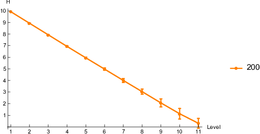
For -Boltzmann samples of structures having signature distance to the target at most , the small entropy of the leaf and the high ratio of the distinguished structure are robust over a range of -values, see Fig. 7. We also observe that, for longer sequences, the entropy is smaller, and therefore the ratio of the distinguished structure is higher.

4.2 Target Identification
Any leaf of the ensemble tree exhibiting a structural entropy less than one, contains, by Proposition 1, a distinguished structure. Successive queries produce a unique, distinguished leaf, which, with high probability, contains structures that are compatible with the queries. Let be the distinguished structure in , and denote the target.
In this section, we shall analyze this probability, , as well as and , see Table 1. For the path identification to the leaf , we consider the error rates and computed in Section 3.1.
As detailed in Section 3.1, these probabilities depend on the error rates and , and since these errors occur independently, we derive , where and denote the number of No-/Yes-answers to queried base pairs along the path, respectively. Fig. 8 displays the distribution of . We observe that has a mean around , i.e., the probabilities of queried base pairs being confirmed and being rejected are roughly equal. For , we have a theoretical estimate . In Fig. 9 we present that decreases as the error rate increases, for fixed .


For (unrestricted) Boltzmann samples generated from random sequences, we present the probability of the leaf containing the target is greater than , which agrees with the above theoretical estimate. Note that this amounts to having no probing data as a constraint for the sampled structures, a worst case scenario, so to speak.
| Quantity | Description |
|---|---|
| the probability of the target being in the leaf | |
| the probability of the distinguished structure being identical to the target | |
| the probability of correctly identifying the target, given that it is in the leaf |
Furthermore, the probability that the distinguished structure is identical to the target is approximately unchanged, see Table 2. indicates, that once we are in the correct leaf, the chance of correctly identifying the target increases to for sequences of length . Accordingly, the key factor is the correct identification of the leaf .
For -Boltzmann samples filtered by signature distance we observe the following: the probability of the leaf to contain the target is greater than is robust over a range of -values, see Fig. 10. As expected, as increases, the probability of the target being in the correct leaf decreases, due to the fact that the -samples become less constraint by the probing data.
In particular, we observe that, for and sequences of length , the probability of the ensemble tree correctly identifying the target in the leaf is greater than , see Fig. 10 (red dashed line). As the Boltzmann ensembles incorporation of probing data via pseudo-energies result in a -value of , this translates into for such ensembles generated by such restricted Boltzmann samplers for sequences of length .
We demonstrate that the ensemble tree localizing the target with high fidelity is robust, across samples of sequences having various lengths and different signature filtration . Fig. 11 (LHS) shows that the ensemble tree for longer sequences has a higher chance of identifying the target. Once we are in the correct leaf, the chance of correctly distinguishing the target significantly increases, from around to over in the case of sequences having nucleotides, see Fig. 11 (RHS).

 |
 |
As mentioned above, the key is the correct identification of the leaf containing the target, and its distinguished structure to coincide with the latter. These events are quantified via and , which depend on the error rates and .
These error rates can be reduced by asking the same query repeatedly. In our Rényi-Ulam game, repeating the same query is tantamount to performing the same experiment multiple times. It is reasonable to assume that experiments are performed independently and thus errors occur randomly. Intuitively, repeated experiments reduce errors originated from the noisy nature of experimental data. Utilizing Bayesian analysis, we show that, if we get the same answer to the query twice, the error rates would become significantly smaller, for example, and , see H.
In principle, we can reduce the error rates by repeating the same query times. The error rates would approach to as grows to infinity. In this case, , i.e. the leaf always contains the target. The fidelity of the distinguished structure increases from to for sequences of length .
5 Discussion
In this paper we propose to enhance the method of identifying the target structure based on RNA probing data. To facilitate this we introduce the framework of ensemble trees in which a sample derived from the partition function of structures is recursively split via queries using information theory. Each query is answered based on either RNA folding data in combination with chemical probing, employing modularity of RNA structures, see Section 3.1 or, alternatively, directly using experimental methods (Mustoe et al. 2019; Cheng et al. 2017). The former type of inference can be viewed as a kind of localization of probing data, relating local to global data by means of structural modularity. We show that within this framework it is possible to identify the target with high fidelity and that this identification requires a small number of base pairs to be queried. In particular we present that, for the Boltzmann ensembles incorporating probing data via pseudo-energies, the probability of the ensemble tree identifying the correct leaf that contains the target is greater than , see Section 4.2.
In our framework, the key factor is the correct identification of the leaf that contains the target. Fig. 12 displays the average base-pair distances 22 2 Here between the target structure and the -th sub-sample on the path. We contrast three scenarios, first the expectation being taken over all ensemble trees (blue), the set of ensemble trees in which the leaf containing the target is identified (green) and its complement (orange). We here present that the correct identification of the leaf containing the target significantly reduces the distance between the target and the sub-samples.

Our framework is based on two assumptions. The first is sampling from the Boltzmann ensemble of structures. This assumption is important, as for an arbitrary sample, the leaf of the ensemble tree does not always contain a distinguished structure. By quantifying the distinguished structure via the flow of entropies of sub-samples on the path, we contrast three classes of samples, the first being a Boltzmann sample (B-sample), the second a uniform sample (U-sample) and the third an E-sample33 3 consisting of different structures with the uniform distribution, each structure containing only one base pair., see Fig. 13. We present that, in a Boltzmann sample, the entropies of sub-samples on the -th level decrease much more sharply than those in the latter two classes, see Fig. 13 (LHS). In particular, the latter two produce leaves exhibiting an average entropy greater than , i.e. not containing a distinguished structure. As proved in Proposition 2, the entropy reduction equals to the entropy of the queried base pair. Fig. 13 (RHS) explains the reason for the significant reduction, that is, the maximum entropy base pairs in Boltzmann samples have entropy close to on each level, implying that the bit queries split the ensemble roughly in half each time. The latter two types of samples do not exhibit this phenomenon.
 |
 |
The second assumption is that the target is contained in the sample. This assumption can be validated by generating samples of larger size, and checking whether or not the distinguished structure is reproducible.
Accordingly, the probability and entropy of a base pair is calculated in the context of the entire ensemble, and thus the ensemble tree together with maximum entropy base pairs. Garcia-Martin and Clote 2015 show that the structural entropy of the entire Boltzmann ensemble is asymptotically linear in , i.e. . Since each queried base pair reduces the entropy by approximately and the reduction is additive by construction, the ensemble tree would require approximately queries to identify a leaf that has entropy smaller than and contains a distinguished structure.


Equipped with the ensemble tree and chemical probing, our framework provides a fragmentation process combining ”local” probing profiles with the ”global” one via modularity. For each queried base pair, our fragmentation subsequently splits the sequence, and determines the presence of base pairs via comparing probing profiles (Section 3.1). Fig. 14 demonstrates the workflow of the fragmentation process, see I. Novikova et al. 2013 developed a different fragmentation method for determining the secondary structure of lncRNAs. Their approach applies chemical probing of the entire RNA, followed by probing of certain overlapping fragments, see Fig. 15. Regions of each fragment exhibiting similar probing profiles are folded independently, and combined in order to obtain the entire structure. At a fundamental level, our fragmentation is different from their approach in that we allow bases from two non-contiguous fragments to pair. Their approach prohibits long-range pairs, such as connecting fragments and in Fig. 15. As a consequence, our method is well suited to deal with the long-range base pairings, whose existence has been shown experimentally (Lai et al. 2018) as well as theoretically (Li and Reidys 2018; Li et al. 2019).
For a sample of RNA pseudoknotted structures, the ensemble tree in our framework can still be computed. However, the structure modularity no longer holds in the pseudoknot case. The reason is that a pseudoknot loop could intersect in more than one base pair with other loops, see Fig. 16 (RHS). The fragmentation with respect to a base pair involved in a pseudoknot could affect several loops, each contributing to the free energy. The change of loop-based energy could lead to splits folding into a different configuration compared to the full transcript. Nevertheless, it would be interesting to find out other experimental methods to facilitate our framework for RNA pseudoknotted structures.
ACKNOWLEDGMENTS We want to thank Christopher Barrett for stimulating discussions and the staff of the Biocomplexity Institute & Initiative at University of Virginia for their great support. We would like to thank Dr. Kevin Weeks for pointing out their recent work (Mustoe et al. 2019). Many thanks to Qijun He, Fenix Huang, Andrei Bura, Ricky Chen, and Reza Rezazadegan for discussions.
AUTHOR DISCLOSURE STATEMENT
The authors declare that no competing financial interests exist.
Appendix A RNA secondary structures
Most computational approaches of RNA structure prediction reduce to a class of coarse grained structures, i.e. the RNA secondary structures (Waterman 1978; Waterman 1979; Smith and Waterman 1978; Howell et al. 1980; Penner and Waterman 1993). These are contact structures via abstracting from the actual spatial arrangement of nucleotides. An RNA secondary structure can be represented as a diagram, a labeled graph over the vertex set whose vertices are arranged in a horizontal line and arcs are drawn in the upper half-plane. Clearly, vertices correspond to nucleotides in the primary sequence and arcs correspond to the Watson-Crick A-U, C-G and wobble U-G base pairs. Two arcs and form a pseudoknot if they cross, i.e. the nucleotides appear in the order in the primary sequence. An RNA secondary structure is a diagram without pseudoknots.
We define two distances for comparing two structures, the base-pair and signature distances.
The base-pair distance utilizes a representation of a secondary structure as a bit string , where denotes the number of all possible base pairs, and is a bit. Given the arc set equipped with the lexicographic order, we define if contains the -th base pair in , otherwise . The base-pair distance between two structures and is the Hamming distance between their corresponding bit strings and .
The - signature (or simply signature) of a structure , is a vector , where when the -th base is unpaired in , otherwise . The signature distance between two structures and is defined as the Hamming distance between their corresponding - signatures and . By construction, the - signature of a secondary structure mimics its probing signals, and the signature distance measures the similarity between the probing profiles of two structures. By observing that each bit corresponds to two base-pairing end, we derive for any and .
Appendix B Energy model
Computational prediction of RNA secondary structures is mainly driven by loop-based energy models (Mathews et al. 1999; Mathews et al. 2004). The key assumption of these approaches is that the free energy of an RNA secondary structure , is estimated by the sum of energy contributions from its individual loops , .
According to thermodynamics, the free energy reflects not only the overall stability of the structure, but also its probability appearing in thermodynamic equilibrium. This leads to the Boltzmann sampling (Ding and Lawrence 2003; Lorenz et al. 2011) of secondary structure based on their equilibrium probabilities, whose computation can be facilitated by the partition function (McCaskill 1990).
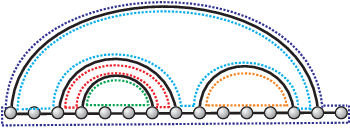
In this model, the energy contribution of a base pair depends on the two adjacent loops that intersect at the base pair, see Fig. 16 (LHS). Note that, in a pseudoknot, since two adjacent loops may intersect at several base pairs, and thus the energy contribution of a base pair could affect several loops, see Fig. 16 (RHS).
 |
 |
Appendix C Chemical probing
The basic idea of RNA structure probing is that chemical probes react differently with paired or unpaired nucleotides. More reactive regions of the RNA are likely to be single stranded and less reactive regions are likely to be base paired. Thus every nucleotide in a folded RNA sequence can be assigned a reactivity score, which depends on the type of chemical or enzymatic footprinting experiments and the strength of the reactivity. It is rarely of absolute certainty, whether or not a specific position is unpaired, or paired; instead, the method produces a probability. The probing data thus produce a vector of probabilities. Several competing methods have been developed to convert the footprinting data for each nucleotide into a probability. Probing data has been further incorporated into RNA folding algorithms by adding a pseudo-energy term, , to the free energy (Deigan et al. 2009; Washietl et al. 2012; Zarringhalam et al. 2012), i.e.
This term engages in the folding process as follows: while positions where structure prediction and experiment data agree with each other are rewarded by a negative pseudo-energy, mismatching locations receive a penalty by way of a positive term. This is tantamount to shifting the partition function in such a way that the equilibrium distribution of structures in favors those that agree with the data.
Appendix D -Boltzmann sampler
Here we incorporate the signature of a target via restricted Boltzmann sampling structures with the signature distance filtration.
We first analyze the signature distances in two classes of Boltzmann samples, one being unrestricted, , and the other being restricted that incorporates the signature of the target via pseudo-energies.
For both types of samples, the distribution of the signature distance between the target and the ensemble is approximately normal, Fig. 17. The means and variances of the normalized signature distance are shown in Table 3. It shows that, while the average signature distance between the target and the unrestricted sampled structure is around , integrating the signature of the target reduces the distance to . This indicates that the incorporation of the signature improves the accuracy of the Boltzmann sampler identifying the target.
 |
 |
The above analysis motivates us to introduce a -Boltzmann sampler for structures with signature distance filtration. For any fraction , let denote the restricted Boltzmann ensemble of structures having signature distance to the target at most , i.e., . The enhanced Boltzmann sampling can be implemented by partition function (McCaskill 1990) and stochastic backtracking technique (Ding and Lawrence 2003), with the augmentation via an additional index recording the signature distance. A complete description of the new sampler will be provided in a future publication. The constraint on the signature distance changes the equilibrium distribution of structures via eliminating those that are inconsistent with signature over certain ratio . Table 3 shows the means and variances of the normalized signature distance for . In particular, we observe that Boltzmann samples incorporating the probing data via pseudo-energies behave similarly as -samples having .
Appendix E State-of-the-art experimental approaches
Determination of base pairs is a fundamental and longstanding problem in RNA biology. A large variety of experimental approaches have been developed to provide reliable solutions to the problem, such as X-ray crystallography, nuclear magnetic resonance (NMR), cryogenic electron microscopy (cryo-EM), chemical and enzymatic probing, cross-linking (Shi 2014; Bothe et al. 2011; Bai et al. 2015; Weeks 2015). Each method has certain strengths and limitations. In particular, chemical probing, as one of the most widely accepted experiments, allows to detect RNA duplexes in vitro and in vivo, and has been combined with high-throughput sequencing to facilitate large-scale analysis on lncRNAs (Weeks 2015). Thus, in the following, we focus on determining the queried base pairs via chemical probing.
Chemical probing data is one-dimensional, i.e. it does not specify base pairing partners. Thus probing data itself does not directly detect base pairings, and any structure information can only be inferred based on compatibility with probing data. Two strategies of structural inference have been developed, correlation analysis and mutate-and-map. Mustoe et al. 2019 introduce PAIR-MaP, which utilizes mutational profiling as a sequencing approach and correlation analysis on profiles. The authors claim that PAIR-MaP provides around accuracy of structure modeling (on average, sensitivity and false discovery rate ). Cheng et al. 2017 introduce M2-seq, a mutate-and-map approach combined with next generation sequencing, which recovers duplexes with a low false discovery rate ().
Appendix F Structural entropy
Proposition 4
Let be a sample of size and be a structure having probability . Then the structural entropy of is bounded by
where
Proof 1
By construction, the multiplicity of in is given by . Since the function is for concave, the structural entropy is maximal in case of all remaining structures being distinct, i.e. each occurs with probability . Therefore
On the other hand, the minimum is achieved when all remaining structures are the same. Thus .
Now we prove Proposition 1.
Proof 2 (Proof of Proposition 1)
Let be the structure having the highest probability in . By Proposition 4, we have
| (3) |
Inspection of the graph of as a function of , we conclude, that for , two solutions of the equation exist, one being for and the other for , see Fig. 18. In case of , we have the unique solution, . Since is monotone over and , inequality (3) implies
We shall proceed by excluding . A contradiction, suppose that and that structures in are arranged in descending order according to their probabilities for . Since each structure in has probability smaller than , the sample contains at least three different structures, i.e. . By construction, we have . Now we consider the following optimization problem
| s.t. | |||
We inspect that the multivariate function reaches its minimum only for and for . In the case of , the minimum cannot be reached and we arrive at some , in contradiction to our assumption . Therefore is the only possible scenario, i.e., contains a distinguished structure with probability at least .

Appendix G Information theory
As the Boltzmann ensemble is a particular type of discrete probability spaces, the information-theoretic results on the ensemble trees will be stated in the more general setup. Let be a discrete probability space consisting of the sample space , its power set as the -algebra and the probability measure . The Shannon entropy of is given by
where the units of are in bits.
A feature is a discrete random variable defined on . Assume that has a finite number of values . Set . The Shannon entropy of the feature is given by
In particular, the values of define a partition of into disjoint subsets , for . This further induces spaces , where the induced distribution is given by
and denotes the probability of having value and is given by
Let denote the conditional entropy of given the value of feature . The entropy gives the expected value of the entropies of the conditional distributions on , averaged over the conditioning feature and can be computed by
Then the entropy reduction of for feature is the difference between the a priori Shannon entropy and the conditional entropy , i.e.
The entropy reduction indicates the change on average in information entropy from a prior state to a state that takes some information as given.
Proof 4 (Proof of Proposition 3)
By definition,
Similarly, we have . Thus is strictly decreasing on and strictly increasing on . Meanwhile, the function is strictly increasing on and symmetric with respect to . Therefore, reaches its minimum when has the maximum value, that is, .
Assertion (2) follows directly from Proposition 2.
Given two features and , we can partition either first by and subsequently by , or first by and then by , or just by a pair of features . In the following, we will show that all three approaches provide the same entropy reduction of .
Before the proof, we define some notations. The joint probability distribution of a pair of features is given by , and the marginal probability distributions are given by and . Clearly, and . The joint entropy of a pair is defined as
The conditional entropy of a feature given is defined as the expected value of the entropies of the conditional distributions , averaged over the conditioning feature , i.e.
Proposition 5 (Chain rule, Cover and Thomas 2006)
| (4) |
Proposition 6
Let denote the entropy reduction of first by the feature and then by the feature , and denote the entropy reduction of by a pair of features . Then
| (5) |
Proof 5
By Proposition 2, we have
Let denote the spaces obtained by partitioning via , i.e. , where , and
where . Then the space is further partitioned into via . That is, , where , and
The entropy reduction is given by the difference between the a priori Shannon entropy and the conditional entropy , which is the expected value of the entropies of , weighted by the probability . In view of Proposition 2, we derive
Eq. (5) follows.
The maximum entropy of an arbitrary feature is achieved when all its outcomes occur with equal probability, and this maximum value is proportional to the logarithm of the number of possible outcomes to the base . Thus Proposition 2 implies that the more possible outcomes a feature has, the higher entropy reduction it could possibly lead to.
Meanwhile, a feature with an arbitrary number of outcomes can be viewed as a combination of binary features, the ones with two possible outcomes. Even though the entropy of the combination of two features is greater than each of them, Proposition 6 shows that partitioning the space subsequently by two features has the same entropy reduction as partitioning by their combination. Therefore, instead of considering features with outcomes as many as possible, we focus on binary features.
Appendix H Query repeats
Here we assess the improvement of the error rates by repeating the same query twice. Let (or ) denote the event of the queried base pair existing (or not) in the target structure. Let (or ) denote the event of the experiment confirming (or rejecting) the base pair. Let denote the event of two independent experiments both rejecting the base pair. Similarly, we have and . Utilizing the same sequences and structures as described in Fig. 3, we estimate the conditional probabilities and . The prior probability can be computed via the expected number of confirmed queried base pairs on the path, divided by the number of queries in each sample. Fig. 8 displays the distribution of having mean around . Thus we adopt . By Bayes’ theorem, we calculate the posterior
where . Since two experiments can be assumed to conditionally independent given and also given , we have and . Similarly, we compute , and etc, see Table 4. It demonstrates that, if we get the same answer to the query twice, the error rates would become significantly smaller, for example, and . In the case of mixed answers or , its probability , i.e., it rarely happens. We would recommend a third experiment and take the majority of three answers when getting two mixed answers.
In principle, we can extend to reducing the error rates by repeating the same query times. The above Bayesian argument is then generalized to sequential updating on the error rates from to . We can show that and approach to , as grows to infinity. In this case, the reliability of the leaf space is , i.e. the leaf always contain the target. The fidelity of the distinguished structure increases from to for sequences of length . To sum up, asking the same query a constant number of times significantly improves the fidelity of the leaf and the distinguished structure.
| Outcome of two experiments | ||
|---|---|---|
| or |
Appendix I A new fragmentation
Here we present a novel fragmentation process, guided by the base-pair queries of the ensemble tree inferred from the restricted Boltzmann sample incorporating chemical probing. Given the maximum entropy base pair, , extraction splits the sequence into two fragments, one being the extracted fragment and the other, , i.e. . We perform probing experiments on these two segments, and obtain the reactive probabilities and , respectively. Let be the reactive probability for the entire sequence, and be the embedding of into , i.e. . As shown in Section 3.1, if the Hamming distance is smaller than threshold , then the probing profiles are similar, i.e. two bases and are paired. Otherwise, they are unpaired in the target structure.
The fragmentation procedure can be summarized as follows:
- 1.
a probing experiment for the entire sequence is performed and the reactive probability is obtained,
- 2.
a Boltzmann sample of structures, consistent with the probing data is computed,
- 3.
the ensemble tree containing the sub-spaces and the corresponding maximum entropy base pairs is constructed,
- 4.
starting with we recursively answer the queries, determining thereby a path through the ensemble tree from the root to a leaf.
- 5.
once in a leaf, Proposition 1 guarantees the existence of a distinctive structure which we stipulate to be the target structure.
References
- Agius et al. (2010) Agius, P., Bennett, K.P., Zuker, M., 2010. Comparing RNA secondary structures using a relaxed base-pair score. RNA 16, 865–878.
- Bai et al. (2015) Bai, X.c., McMullan, G., Scheres, S.H.W., 2015. How cryo-EM is revolutionizing structural biology. Trends in Biochemical Sciences 40, 49–57.
- Berlekamp (1968) Berlekamp, E.R., 1968. Block coding for the binary symmetric channel with noiseless, delayless feedback, in: Mann, H.B. (Ed.), Error correcting codes: proceedings of a symposium, Wiley, New York. pp. 61–88.
- Bothe et al. (2011) Bothe, J.R., Nikolova, E.N., Eichhorn, C.D., Chugh, J., Hansen, A.L., Al-Hashimi, H.M., 2011. Characterizing RNA dynamics at atomic resolution using solution-state NMR spectroscopy. Nature Methods 8, 919–931.
- Cheng et al. (2017) Cheng, C.Y., Kladwang, W., Yesselman, J.D., Das, R., 2017. RNA structure inference through chemical mapping after accidental or intentional mutations. Proceedings of the National Academy of Sciences 114, 9876–9881.
- Cover and Thomas (2006) Cover, T.M., Thomas, J.A., 2006. Elements of Information Theory (Wiley Series in Telecommunications and Signal Processing). Wiley-Interscience.
- Deigan et al. (2009) Deigan, K.E., Li, T.W., Mathews, D.H., Weeks, K.M., 2009. Accurate SHAPE-directed RNA structure determination. Proceedings of the National Academy of Sciences 106, 97–102.
- Ding and Lawrence (2003) Ding, Y., Lawrence, C.E., 2003. A statistical sampling algorithm for RNA secondary structure prediction. Nucleic Acids Research 31, 7280–7301.
- Garcia-Martin and Clote (2015) Garcia-Martin, J.A., Clote, P., 2015. RNA thermodynamic structural entropy. PLOS ONE 10, e0137859.
- Hajdin et al. (2013) Hajdin, C.E., Bellaousov, S., Huggins, W., Leonard, C.W., Mathews, D.H., Weeks, K.M., 2013. Accurate SHAPE-directed RNA secondary structure modeling, including pseudoknots. Proceedings of the National Academy of Sciences 110, 5498–5503.
- Howell et al. (1980) Howell, J., Smith, T., Waterman, M., 1980. Computation of Generating Functions for Biological Molecules. SIAM J. Appl. Math. 39, 119–133.
- Lai et al. (2018) Lai, W.J.C., Kayedkhordeh, M., Cornell, E.V., Farah, E., Bellaousov, S., Rietmeijer, R., Salsi, E., Mathews, D.H., Ermolenko, D.N., 2018. mRNAs and lncRNAs intrinsically form secondary structures with short end-to-end distances. Nature Communications 9.
- Li et al. (2019) Li, T.J.X., Burris, C.S., Reidys, C.M., 2019. The block spectrum of RNA pseudoknot structures. Journal of Mathematical Biology 79, 791–822.
- Li and Reidys (2018) Li, T.J.X., Reidys, C.M., 2018. The Rainbow Spectrum of RNA Secondary Structures. Bull. Math. Biol. 80, 1514–1538.
- Lorenz et al. (2011) Lorenz, R., Bernhart, S., Höner zu Siederdissen, C., Tafer, H., Flamm, C., Stadler, P., Hofacker, I., 2011. ViennaRNA Package 2.0. Algorithms Mol. Biol. 6, 26.
- Mathews et al. (1999) Mathews, D., Sabina, J., Zuker, M., Turner, D., 1999. Expanded sequence dependence of thermo-dynamic parameters improves prediction of RNA secondary structure. J. Mol. Biol. 288, 911–940.
- Mathews et al. (2004) Mathews, D.H., Disney, M.D., Childs, J.L., Schroeder, S.J., Zuker, M., Turner, D.H., 2004. Incorporating chemical modification constraints into a dynamic programming algorithm for prediction of RNA secondary structure. Proceedings of the National Academy of Sciences of the United States of America 101, 7287–7292.
- McCaskill (1990) McCaskill, J., 1990. The equilibrium partition function and base pair binding probabilities for RNA secondary structure. Biopolymers 29, 1105–1119.
- Merino et al. (2005) Merino, E.J., Wilkinson, K.A., Coughlan, J.L., Weeks, K.M., 2005. RNA structure analysis at single nucleotide resolution by selective 2?-hydroxyl acylation and primer extension (SHAPE). Journal of the American Chemical Society 127, 4223–4231.
- Mustoe et al. (2019) Mustoe, A.M., Lama, N., Irving, P.S., Olson, S.W., Weeks, K.M., 2019. RNA base pairing complexity in living cells visualized by correlated chemical probing. bioRxiv , 596353.
- Novikova et al. (2013) Novikova, I.V., Dharap, A., Hennelly, S.P., Sanbonmatsu, K.Y., 2013. 3s: Shotgun secondary structure determination of long non-coding RNAs. Methods 63, 170–177.
- Pelc (1989) Pelc, A., 1989. Searching with known error probability. Theoretical Computer Science 63, 185–202.
- Penner and Waterman (1993) Penner, R., Waterman, M., 1993. Spaces of RNA secondary structures. Adv. Math. 217, 31–49.
- Rényi (1961) Rényi, A., 1961. On a problem of information theory. MTA Mat. Kut. Int. Kozl. 6, 505–516.
- Rivest et al. (1980) Rivest, R.L., Meyer, A.R., Kleitman, D.J., Winklmann, K., Spencer, J., 1980. Coping with errors in binary search procedures. Journal of Computer and System Sciences 20, 396–404.
- Shannon (1948) Shannon, C.E., 1948. A mathematical theory of communication. The Bell System Technical Journal 27, 379–423.
- Shi (2014) Shi, Y., 2014. A glimpse of structural biology through x-ray crystallography. Cell 159, 995–1014.
- Smith and Waterman (1978) Smith, T.F., Waterman, M.S., 1978. RNA secondary structure. Math. Biol. 42, 31–49.
- Spencer (1992) Spencer, J., 1992. Ulam’s searching game with a fixed number of lies. Theoretical Computer Science 95, 307–321.
- Stern et al. (1988) Stern, S., Moazed, D., Noller, H.F., 1988. Structural analysis of RNA using chemical and enzymatic probing monitored by primer extension, in: Methods in Enzymology. Academic Press. volume 164 of Ribosomes, pp. 481–489.
- Sükösd et al. (2013) Sükösd, Z., Knudsen, B., Anderson, J.W., Novák, A., Kjems, J., Pedersen, C.N., 2013. Characterising RNA secondary structure space using information entropy. BMC Bioinformatics 14, S22.
- Ulam (1976) Ulam, S., 1976. Adventures of a Mathematician. Scribner, New York.
- Washietl et al. (2012) Washietl, S., Hofacker, I.L., Stadler, P.F., Kellis, M., 2012. RNA folding with soft constraints: reconciliation of probing data and thermodynamic secondary structure prediction. Nucleic Acids Research 40, 4261–4272.
- Waterman (1978) Waterman, M., 1978. Secondary structure of single-stranded nucleic acids, in: Rota, G.C. (Ed.), Studies on foundations and combinatorics, Advances in mathematics supplementary studies, Academic Press N.Y.. pp. 167–212.
- Waterman (1979) Waterman, M., 1979. Combinatorics of RNA Hairpins and Cloverleaves. Stud. Appl. Math. 60, 91–98.
- Weeks (2015) Weeks, K.M., 2015. Review toward all RNA structures, concisely. Biopolymers 103, 438–448.
- Zarringhalam et al. (2012) Zarringhalam, K., Meyer, M.M., Dotu, I., Chuang, J.H., Clote, P., 2012. Integrating chemical footprinting data into RNA secondary structure prediction. PLOS ONE 7, e45160.
- Zuker (1989) Zuker, M., 1989. On finding all suboptimal foldings of an RNA molecule. Science 244, 48–52.
- Zuker and Sankoff (1984) Zuker, M., Sankoff, D., 1984. RNA secondary structures and their prediction. Bulletin of Mathematical Biology 46, 591–621.