Estimation and Applications of Quantile Regression for Binary Longitudinal DataJournal: Advances in Econometrics

Mohammad Arshad Rahman Address: Department of Economic Sciences, Indian Institute of Technology Kanpur Note: Room 672, Faculty Building, IIT Kanpur, Kanpur 208016, India; email: marshad@iitk.ac.in. Angela Vossmeyer Address: Robert Day School of Economics and Finance, Claremont McKenna College Note: Robert Day School of Economics and Finance, Claremont McKenna College, 500 E. Ninth St., Claremont, CA 91711; email: angela.vossmeyer@cmc.edu.

Abstract

This paper develops a framework for quantile regression in binary longitudinal data settings. A novel Markov chain Monte Carlo (MCMC) method is designed to fit the model and its computational efficiency is demonstrated in a simulation study. The proposed approach is flexible in that it can account for common and individual-specific parameters, as well as multivariate heterogeneity associated with several covariates. The methodology is applied to study female labor force participation and home ownership in the United States. The results offer new insights at the various quantiles, which are of interest to policymakers and researchers alike.

Keywords:

Bayesian inference, Binary outcomes, Female labor force participation, Home ownership, Limited dependent variables, Panel data.

The authors thank the anonymous referees, Ivan Jeliazkov, David Brownstone, John Geweke, K.L. Krishna, Antonio Galvao, Michael Guggisberg, and Editor Justin Tobias for their helpful comments. Discussions and suggestions from the participants at the Winter School, Delhi School of Economics (2017) and Advances in Econometrics Conference (2018) are appreciated. A special thanks to Dale Poirier for sharing the Reverend’s insights and teaching us the controversy.

1 Introduction

The proliferation of panel data studies is well-documented and much of it has been attributed to data availability and challenging methodology (Hsiao 2007). While panel data has been attractive for understanding behavior and dynamics, the modeling complexities involved in it have moved attention away from its unique capacities. Modeling features such as a binary outcome variable or a quantile analysis, which are relatively straightforward to implement with cross-sectional data, are challenging and computationally burdensome for panel data. However, these features are important as they allow for the modeling of probabilities and lead to a richer view of how the covariates influence the outcome variable. Motivated by these difficulties, this paper adds to the methodological advancements for panel data by developing quantile regression methods for binary longitudinal data and designing a computationally efficient estimation algorithm. The approach is applied to two empirical studies, female labor force participation and home ownership.

The paper touches on three growing econometric literatures – discrete panel data, quantile regression for panel data, and quantile regression for discrete data. In reference to the latter, quantile regression has been implemented in binary data models (Kordas 2006; Benoit and Poel 2012), ordered data models (Rahman 2016; Alhamzawi and Ali 2018), count data models (Machado and Silva 2005; Harding and Lamarche 2015), and censored data models (Portnoy 2003; Harding and Lamarche 2012). For limited dependent variables, the concern is modeling the latent utility differential in the quantile framework, since the response variable takes limited values and does not yield continuous quantiles. Our paper follows the work in this literature by using the latent utility setting and interpreting the utility as a “propensity” or “willingness” that underlie the latent scale, thus increasing our understanding of the impact of the covariates on the binary outcomes.

The literature on quantile regression in panel data settings includes (but is not limited to) Koenker 2004, Geraci and Bottai 2007, Liu and Bottai 2009, Galvao 2010, Galvao and Kato 2016, Lamarche 2010, Harding and Lamarche 2009 and Harding and Lamarche 2017. The latter of these papers discusses the issues associated with solely focusing on fixed effects estimators and highlights the usefulness of allowing for a flexible specification of individual heterogeneity associated with covariates, also of interest in the present paper. In a recent Bayesian paper, Luo et al. 2012 develop a hierarchical model to estimate the parameters of conditional quantile functions with random effects. The authors do so by adopting an Asymmetric Laplace (AL) distribution for the residual errors and suitable prior distributions for the parameters. However, directly using the AL distribution does not yield tractable conditional densities for all of the parameters and hence a combination of Metropolis-Hastings (MH) and Gibbs sampling is required for model estimation. The use of the MH algorithm may require tuning at each quantile. To overcome this limitation, Luo et al. 2012 also present a full Gibbs sampling algorithm that utilizes the normal-exponential mixture representation of the AL distribution. This mixture representation is also followed in our work, with important computational improvements.

Finally, for discrete panel data, recent work by Bartolucci and Nigro 2010 introduces a quadratic exponential model for binary panel data and utilizes a conditional likelihood approach, which is computationally simpler than previous classical estimators. Bayesian approaches to binary panel data models include work by Albert and Chib 1996, Chib and Carlin 1999, Chib and Jeliazkov 2006, and Burda and Harding 2013. These work influence the estimation methods designed in our quantile approach to binary panel data.

This paper contributes to the three literatures by extending the various methodologies to a hierarchical Bayesian quantile regression model for binary longitudinal data and proposing a Markov chain Monte Carlo (MCMC) algorithm to estimate the model. The model handles both common (fixed) and individual-specific (random) parameters (commonly referred to mixed effects in statistics). The algorithm implements a blocking procedure that is computationally efficient and the distributions involved allow for straightforward calculations of covariate effects. The framework is implemented in two empirical applications. The first application examines female labor force participation, which has been heavily studied in panel form. The topic became of particular interest in the state dependence versus heterogeneity debate (Heckman 1981a). We revisit this question and implement our panel quantile approach, which has been otherwise unexplored for this topic. The results offer new insights regarding the determinants of female labor force participation and how the ages of children have different effects across the quantiles and utility scale. The findings suggest that policy should be focused on women’s transitions into the labor force after child birth and the few years after.

The second application considers the probability of home ownership during the Great Recession. Micro-level empirical analyses on individuals moving into and out of housing markets are lacking in the recent literature. Past studies include Carliner 1974 and Poirier 1977, but the recent housing crisis offers a new opportunity to reevaluate the topic. Furthermore, a full quantile analysis of home ownership is yet to be explored. Since home ownership is a choice that requires years of planning, individual characteristics may range drastically across the latent utility scale. The analysis presented in this paper controls for multivariate heterogeneity in individuals and wealth, and investigates the determinants of home ownership, state dependence in home ownership, and how the shock to housing markets affected these items. The results provide an understanding as to how individuals of particular demographics and socioeconomic status fared during the collapse of the housing market.

The rest of the paper is organized as follows. Section 2 reviews quantile regression and the AL distribution, Section 3 introduces the quantile regression model for binary longitudinal data, presents a simulation study, and discusses methods for covariate effects. Section 4 considers the two applications and concluding remarks are offered in Section 5.

2 Quantile Regression and Asymmetric Laplace Distribution

The $p$ -th quantile of a random variable $Y$ is the value $y_{0}$ such that the probability that $Y$ will be less than $y_{0}$ equals $p\in(0,1)$ . Mathematically, if $Q(\cdot)$ denotes the inverse of the cumulative distribution function (cdf) of $Y$ , the $p$ -th quantile is defined as

Q_{Y}(p)\equiv F_{Y}^{-1}(p)=\mathrm{inf}\{y_{0}:F(y_{0})\geq p\}.

Quantile regression implements the idea of quantiles within the regression framework with $Q(\cdot)$ modified to denote the inverse cdf of the dependent variable given the covariates. The objective is to estimate conditional quantile functions and to this purpose, regression quantiles are estimated by minimizing the quantile objective function which is a sum of asymmetrically weighted absolute residuals.

To formally explain the quantile regression problem, consider the following linear model,

y_{i}=x^{\prime}_{i}\beta_{p}+\varepsilon_{i},\qquad\mathrm{with}\qquad Q_{\varepsilon_{i}}(p|x_{i})=0,

(1)

where $y_{i}$ is a scalar response variable, $x_{i}$ is a $k\times 1$ vector of covariates, $\beta_{p}$ is a $k\times 1$ vector of unknown parameters that depend on quantile $p$ , and $\varepsilon_{i}$ is the error term such that its $p$ -th quantile equals zero. Henceforth, we will drop the subscript $p$ for notational simplicity. In classical econometrics, the error $\varepsilon$ does not (or is not assumed to) follow any distribution and estimation requires minimizing the following objective function,

\min_{\beta\in\mathbf{R}^{k}}\bigg[\;\sum_{i:y_{i}<x_{i}^{\prime}\beta}(1-p)\;|y_{i}-x_{i}^{\prime}\beta|\;\;+\sum_{i:y_{i}\geq x_{i}^{\prime}\beta}p\;|y_{i}-x_{i}^{\prime}\beta|\;\;\bigg].

(2)

The minimizer $\hat{\beta}$ gives the $p$ -th regression quantile and the estimated conditional quantile function is obtained as $\hat{y}_{i}=x^{\prime}_{i}\hat{\beta}$ . Alternatively, the objective function (2) can be written as a sum of piecewise linear or check functions as follows,

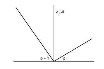
\min_{\beta\in\mathbf{R}^{k}}\sum_{i=1}^{n}\rho_{p}(y_{i}-x^{\prime}_{i}\beta),

where $\rho_{p}(u)=u\cdot(p-I(u<0))$ and $I(\cdot)$ is an indicator function, which equals 1 if the condition inside the parenthesis is true and 0 otherwise. The check function, as seen in Figure 1, is not differentiable at the origin. Hence, classical econometrics relies on computational techniques to estimate quantile regression models. Such computational methods include the simplex algorithm (Dantzig 1963; Dantzig and Thapa 1997; Dantzig and Thapa 2003; Barrodale and Roberts 1973; Koenker and d’Orey 1987), the interior point algorithm (Karmarkar 1984; Mehrotra 1992; Portnoy and Koenker 1997), the smoothing algorithm (Madsen and Nielsen 1993; Chen 2007), and metaheuristic algorithms (Rahman 2013).

Refer to caption — Figure 1: Quantile regression check function

In contrast to classical quantile regression, Bayesian quantile regression assumes that the error follows an AL distribution because the AL pdf contains the quantile loss function (2) in its exponent. This facilitates the construction of a working likelihood, required for Bayesian analysis. Maximizing an AL likelihood is equivalent to minimizing the quantile objective function (Koenker and Machado 1999; Yu and Moyeed 2001). A random variable $Y$ follows an AL distribution if its probability density function (pdf) is given by:

f(y|\mu,\sigma,p)=\frac{p(1-p)}{\sigma}\exp\bigg[-\rho_{p}\bigg(\frac{y-\mu}{\sigma}\bigg)\bigg],

(3)

where $\rho_{p}(\cdot)$ is the check function as defined earlier, $-\infty<\mu<\infty$ is the location parameter, $\sigma>0$ is the scale parameter, and $0<p<1$ is the skewness parameter (Kotz et al. 2001; Yu and Zhang 2005). The mean and variance of $Y$ with pdf (3) are

E(Y)=\mu+\frac{\sigma(1-2p)}{p(1-p)}\quad\textrm{and}\quad V(Y)=\frac{\sigma^{2}(1-2p+2p^{2})}{p^{2}(1-p)^{2}}.

If $\mu=0$ and $\sigma=1$ , then both mean and variance depend only on $p$ and hence are fixed for a given value of $p$ .

The Bayesian approach to quantile regression for binary data assumes that $\varepsilon\sim AL(0,1,p)$ . Here, the variance is constant to serve as a normalization for identification, typical in probit and logit models (Poirier and Ruud 1988; Koop and Poirier 1993; Jeliazkov and Rahman 2012). However, working directly with the AL distribution is not conducive to constructing a Gibbs sampler and hence the normal-exponential mixture of the AL distribution is often employed (Kozumi and Kobayashi 2011). Several recent papers have utilized the mixture representation, including Ji et al. 2012 for Bayesian model selection in binary and Tobit quantile regression, Luo et al. 2012 for estimating linear longitudinal data models, and Rahman 2016 for estimating ordinal quantile regression models. We also exploit the normal-exponential mixture representation of the AL distribution to derive the estimation algorithm for quantile regression in binary longitudinal data settings.

3 The Quantile Regression Model for Binary Longitudinal Data

This section presents the quantile regression model for binary longitudinal data (QBLD) and an estimation algorithm to fit the model. The performance of the proposed algorithm is illustrated in a simulation study. The last part of this section considers methods for model comparison and covariate effects.

3.1 The Model

The proposed model looks at quantiles of binary longitudinal data expressed as a function of covariates with common effects and individual-specific effects. The individual-specific effects offer additional flexibility in that both intercept and slope heterogeneity can be captured, which are important to avoid biases in the parameter estimates. The QBLD model can be conveniently expressed in the latent variable formulation (Albert and Chib 1993) as follows,

\begin{split}z_{it}&=x^{\prime}_{it}\beta+s^{\prime}_{it}\alpha_{i}+\varepsilon_{it},\hskip 36.135pt\forall\;i=1,\cdots,n,\;\;t=1,\cdots,T_{i},\\ y_{it}&=\left\{\begin{array}[]{ll}1&\textrm{if}\;z_{it}>0,\\ 0&\textrm{otherwise},\end{array}\right.\end{split}

(4)

where the latent variable $z_{it}$ denotes the value of $z$ at the $t$ -th time period on the $i$ -th individual, $x^{\prime}_{it}$ is a $1\times k$ vector of explanatory variables, $\beta$ is $k\times 1$ vector of common parameters, $s^{\prime}_{it}$ is a $1\times l$ vector of covariates that have individual-specific effects, $\alpha_{i}$ is an $l\times 1$ vector of individual-specific parameters, and $\varepsilon_{it}$ is the error term assumed to be independently distributed as $AL(0,1,p)$ with $Q_{\varepsilon_{it}}(p|x_{it},\alpha_{i})=0$ . This implies that the conditional density of $z_{it}|\alpha_{i}$ is an $AL(x^{\prime}_{it}\beta+s^{\prime}_{it}\alpha_{i},1,p)$ for $i=1,\cdots,n$ , and $t=1,\cdots,T_{i}$ , with $Q_{z_{it}}(p|x_{it},\alpha_{i})=x^{\prime}_{it}\beta+s^{\prime}_{it}\alpha_{i}$ . Note that $s_{it}$ may contain a constant for intercept heterogeneity, as well as other covariates (which are often a subset of those in $x_{it}$ ) to account for slope heterogeneity of those variables. The variable $z_{it}$ is unobserved and represents the latent utility associated with the observed binary choice $y_{it}$ . The latent variable formulation serves as a convenient tool in the estimation process (Albert and Chib 1993). Furthermore, latent utility underlies the interpretation of the results at the various quantiles.

While working directly with the AL density is an option, the resulting posterior will not yield the full set of tractable conditional distributions necessary for a Gibbs sampler. Thus, we utilize the normal-exponential mixture representation of the AL distribution, presented in Kozumi and Kobayashi 2011, and express the error as follows,

\varepsilon_{it}=\theta w_{it}+\tau\sqrt{w_{it}}\,u_{it},\hskip 54.2025pt\forall\;i=1,\cdots,n;\;t=1,\cdots,T_{i},

(5)

where $u_{it}\sim N(0,1)$ is mutually independent of $w_{it}\sim\mathcal{E}(1)$ with $\mathcal{E}$ representing an exponential distribution and the constants $\theta=\frac{1-2p}{p(1-p)}$ and $\tau=\sqrt{\frac{2}{p(1-p)}}$ . The mixture representation gives access to the appealing properties of the normal distribution.

Longitudinal data models often involve a moderately large amount of data, so it is important to take advantage of any opportunity to reduce the computational burden. One such trick is to stack the model for each individual $i$ (Hendricks et al. 1979). We define $z_{i}=(z_{i1},\cdots,z_{iT_{i}})^{\prime}$ , $X_{i}=(x^{\prime}_{i1},\cdots,x^{\prime}_{iT_{i}})^{\prime}$ , $S_{i}=(s^{\prime}_{i1},\cdots,s^{\prime}_{iT_{i}})^{\prime}$ , $w_{i}=(w_{i1},\cdots,w_{iT_{i}})^{\prime}$ , $D_{\tau\sqrt{w_{i}}}=\mathrm{diag}(\tau\sqrt{w_{i1}},\cdots,\tau\sqrt{w_{iT_{i}}})$ , and $u_{i}=(u_{i1},\cdots,u_{iT_{i}})^{\prime}$ . Building on equations (4) and (5), the resulting hierarchical model can be written as,

\begin{split}z_{i}&=X_{i}\beta+S_{i}\alpha_{i}+\theta w_{i}+D_{\tau\sqrt{w_{i}}}\;u_{i},\\ y_{it}&=\left\{\begin{array}[]{ll}1&\textrm{if}\;z_{it}>0,\\ 0&\textrm{otherwise},\end{array}\right.\\ \alpha_{i}|\varphi^{2}&\sim N_{l}(0,\varphi^{2}I_{l}),\hskip 43.36243ptw_{it}\sim\mathcal{E}(1),\hskip 43.36243ptu_{it}\sim N(0,1),\\ \beta&\sim N_{k}(\beta_{0},B_{0}),\quad\varphi^{2}\sim IG(c_{1}/2,d_{1}/2),\end{split}

(6)

where we assume that $\alpha_{i}$ are identically distributed as a normal distribution. The last row represents the prior distributions with $N$ and $IG$ denoting the normal and inverse-gamma distributions, respectively. Here, we note that the form of the prior distribution on $\beta$ holds a penalty interpretation on the quantile loss function (Koenker 2004). A normal prior on $\beta$ implies a $\ell_{2}$ penalty and has been used in Yuan and Yin 2010, and Luo et al. 2012. One may also employ a Laplace prior distribution on $\beta$ that imposes $\ell_{1}$ penalization, as used in several articles such as Alhamzawi and Ali 2018. While Alhamzawi and Ali 2018 also work with quantile regression for discrete panel data (ordered, in particular), our work contributes by considering multivariate heterogeneity (not just intercept heterogeneity), and introducing computational improvements outlined below.

By Bayes’ theorem, we express the “complete joint posterior” density as proportional to the product of likelihood function and the prior distributions as follows,

\begin{split}\pi(\beta,\alpha,w,z,\varphi^{2}|y)&\propto\bigg\{\prod_{i=1}^{n}f(y_{i}|z_{i},\beta,\alpha_{i},w_{i},\varphi^{2})\pi(z_{i}|\beta,\alpha_{i},w_{i})\pi(w_{i})\pi(\alpha_{i}|\varphi^{2})\bigg\}\pi(\beta)\pi(\varphi^{2}),\\ &\propto\bigg\{\prod_{i=1}^{n}\bigg[\prod_{t=1}^{T_{i}}f(y_{it}|z_{it})\bigg]\pi(z_{i}|\beta,\alpha_{i},w_{i})\pi(w_{i})\pi(\alpha_{i}|\varphi^{2})\bigg\}\pi(\beta)\pi(\varphi^{2}),\end{split}

(7)

where the first line uses independence between prior distributions and second line follows from the fact that given $z_{it}$ , the observed $y_{it}$ is independent of all parameters because the second line of (6) determines $y_{it}$ given $z_{it}$ with probability 1. Substituting the distribution of the variables associated with the likelihood and the prior distributions in (7) yields the following expression,

	$\displaystyle\pi(\beta,\alpha,w,z,\varphi^{2}\|y)\propto\bigg\{\prod_{i=1}^{n}\prod_{t=1}^{T_{i}}\Big[I(z_{it}>0)I(y_{it}=1)+I(z_{it}\leq 0)I(y_{it}=0)\Big]\bigg\}$
	$\displaystyle\hskip 7.22743pt\times\exp\Big[-\frac{1}{2}\sum_{i=1}^{n}\Big\{(z_{i}-X_{i}\beta-S_{i}\alpha_{i}-\theta w_{i})^{\prime}\,D_{\tau\sqrt{w_{i}}}^{-2}\,(z_{i}-X_{i}\beta-S_{i}\alpha_{i}-\theta w_{i})\Big\}\Big]$
	$\displaystyle\hskip 7.22743pt\times\bigg\{\prod_{i=1}^{n}\|D_{\tau\sqrt{w_{i}}}^{2}\|^{-\frac{1}{2}}\bigg\}\times\exp\bigg(-\sum_{i=1}^{n}\sum_{t=1}^{T_{i}}w_{it}\bigg)\big(2\pi\varphi^{2}\big)^{-\frac{nl}{2}}\exp\Big[-\frac{1}{2\varphi^{2}}\sum_{i=1}^{n}\alpha^{\prime}_{i}\alpha_{i}\Big]$		(8)
	$\displaystyle\hskip 7.22743pt\times(2\pi)^{-\frac{k}{2}}\|B_{0}\|^{-\frac{1}{2}}\exp\Big[-\frac{1}{2}(\beta-\beta_{0})^{\prime}B_{0}^{-1}(\beta-\beta_{0})\Big]\times(\varphi^{2})^{-(\frac{c_{1}}{2}+1)}\exp\Big[-\frac{d_{1}}{2\varphi^{2}}\Big].$

The joint posterior density (8) does not have a tractable form, and thus simulation techniques are necessary for estimation. Bayesian methods are increasing in popularity (Poirier 2006), and this paper takes the approach for a couple of reasons. First, with discrete panel data, working with the likelihood function is complicated because it is analytically intractable. The inclusion of individual-specific effects makes matters worse. Second, while numerical simulation methods are available for discrete panel data, they are often slow and difficult to implement (Burda and Harding 2013). The availability of a full set of conditional distributions (which are outlined below) makes Gibbs sampling an attractive option that will be simpler to implement, both conceptually and computationally.

We can derive the conditional posteriors of the parameters and latent variables by a straightforward extension of the estimation technique for the linear mixed-effects model presented in Luo et al. 2012. This is presented as Algorithm 2 in Appendix A, which shows the conditional posterior distributions for the parameters and latent variables necessary for a Gibbs sampler. While this Gibbs sampler is straightforward, there is potential for poor mixing properties due to correlation between $(\beta,\alpha_{i})$ and $(z_{i},\alpha_{i})$ . The correlation often arises because the variables corresponding to the parameters in $\alpha_{i}$ are often a subset of those in $x_{it}$ . Thus, by conditioning these items on one another, the mixing of the Markov chain will be slow.

Algorithm 1 (Blocked Sampling)

Sample $(\beta,z_{i})$ in one block. The objects $(\beta,z_{i})$ are sampled in the following two sub-steps.

(a)

Let $\Omega_{i}=\left(\varphi^{2}S_{i}S^{\prime}_{i}+D_{\tau\sqrt{w_{i}}}^{2}\right)$ . Sample $\beta$ marginally of $\alpha$ from $\beta|z,w,\varphi^{2}$ $\sim$ $N(\tilde{\beta},\tilde{B})$ , where,

\tilde{B}^{-1}=\bigg(\sum_{i=1}^{n}X^{\prime}_{i}\Omega_{i}^{-1}X_{i}+B_{0}^{-1}\bigg)\hskip 4.62497pt\mathrm{and}\hskip 4.62497pt\tilde{\beta}=\tilde{B}\left(\sum_{i=1}^{n}X^{\prime}_{i}\Omega_{i}^{-1}(z_{i}-\theta w_{i})+B_{0}^{-1}\beta_{0}\right).

(b)

Sample the vector $z_{i}|y_{i},\beta,w_{i},\varphi^{2}\sim TMVN_{B_{i}}(X_{i}\beta+\theta w_{i},\Omega_{i})$ for all $i=1,\cdots,n$ , where $B_{i}=(B_{i1}\times B_{i2}\times\ldots\times B_{iT_{i}})$ and $B_{it}$ is the interval $(0,\infty)$ if $y_{it}=1$ and the interval $(-\infty,0]$ if $y_{it}=0$ . This is done by sampling $z_{i}$ at the $j$ -th pass of the MCMC iteration using a series of conditional posterior distribution as follows:

z_{it}^{j}|z_{i1}^{j},\cdots,z_{i(t-1)}^{j},z_{i(t+1)}^{j},\cdots,z_{iT_{i}}^{j}\sim TN_{B_{it}}(\mu_{t|-t},\Sigma_{t|-t}),\hskip 36.135pt\mathrm{for}\;t=1,\cdots,T_{i},

where $TN$ denotes a truncated normal distribution. The terms $\mu_{t|-t}$ and $\Sigma_{t|-t}$ are the conditional mean and variance, respectively, and are defined as,

	$\displaystyle\mu_{t\|-t}$	$\displaystyle=$	$\displaystyle x^{\prime}_{it}\beta+\theta w_{it}+\Sigma_{t,-t}\Sigma_{-t,-t}^{-1}\big(z_{i,-t}^{j}-(X_{i}\beta+\theta w_{i})_{-t}\big),$
	$\displaystyle\Sigma_{t\|-t}$	$\displaystyle=$	$\displaystyle\Sigma_{t,t}-\Sigma_{t,-t}\Sigma_{-t,-t}^{-1}\Sigma_{-t,t},$

where $z_{i,-t}^{j}=(z_{i1}^{j},\cdots,z_{i(t-1)}^{j},z_{i(t+1)}^{j-1},\cdots,z_{iT_{i}}^{j-1})$ , $(X_{i}\beta+\theta w_{i})_{-t}$ is a column vector with $t$ -th element removed, $\Sigma_{t,t}$ denotes the $(t,t)$ -th element of $\Omega_{i}$ , $\Sigma_{t,-t}$ denotes the $t$ -th row of $\Omega_{i}$ with element in the $t$ -th column removed and $\Sigma_{-t,-t}$ is the $\Omega_{i}$ matrix with $t$ -th row and $t$ -th column removed.

Sample $\alpha_{i}|z,\beta,w,\varphi^{2}$ $\sim$ $N(\tilde{a},\tilde{A})$ for $i=1,\cdots,n$ , where,

\tilde{A}^{-1}=\left(S^{\prime}_{i}\,D^{-2}_{\tau\sqrt{w_{i}}}\,S_{i}+\frac{1}{\varphi^{2}}I_{l}\right)\hskip 9.24994pt\mathrm{and}\hskip 9.24994pt\tilde{a}=\tilde{A}\left(S^{\prime}_{i}D^{-2}_{\tau\sqrt{w_{i}}}\,\big(z_{i}-X_{i}\beta-\theta w_{i}\big)\right).

Sample $w_{it}|z_{it},\beta,\alpha_{i}$ $\sim$ $GIG\,(0.5,\tilde{\lambda}_{it},\tilde{\eta})$ for $i=1,\cdots,n$ and $t=1,\cdots,T_{i}$ , where,

\tilde{\lambda}_{it}=\bigg(\frac{z_{it}-x^{\prime}_{it}\beta-s^{\prime}_{it}\alpha_{i}}{\tau}\bigg)^{2}\hskip 9.24994pt\mathrm{and}\hskip 9.24994pt\tilde{\eta}=\bigg(\frac{\theta^{2}}{\tau^{2}}+2\bigg).

4.

Sample $\varphi^{2}|\alpha\sim IG(\tilde{c}_{1}/2,\tilde{d}_{1}/2)$ , where $\tilde{c}_{1}=\Big(nl+c_{1}\Big)$ and $\tilde{d}_{1}=\Big(\displaystyle\sum_{i=1}^{n}\alpha_{i}^{\prime}\alpha_{i}+d_{1}\Big)$ .

To avoid this issue, we develop an alternative algorithm which jointly samples $(\beta,z_{i})$ in one block within the Gibbs sampler. This blocked approach significantly improves the mixing properties of the Markov chain. The success of these blocking techniques can be found in Liu 1994, Chib and Carlin 1999, and Chib and Jeliazkov 2006. The details of our blocked sampler are described in Algorithm 1.¹¹ 1 The derivation of the conditional posterior densities are presented in Appendix B. In particular, $\beta$ is sampled marginally of $\alpha_{i}$ from a multivariate normal distribution. The latent variable $z_{i}$ is sampled marginally of $\alpha_{i}$ from a truncated multivariate normal distribution denoted by $TMVN_{B_{i}}$ , where $B_{i}$ is the truncation region given by $B_{i}=(B_{i1}\times B_{i2}\times\ldots\times B_{iT_{i}})$ such that $B_{it}$ is the interval $(0,\infty)$ if $y_{it}=1$ and the interval $(-\infty,0]$ if $y_{it}=0$ . To draw from a truncated multivariate normal distribution, we utilize the method proposed in Geweke 1991. This involves drawing from a series of conditional posteriors which are univariate truncated normal distributions. Previous work using this approach include Chib and Greenberg 1998 and Chib and Carlin 1999. The random effects parameter $\alpha_{i}$ is sampled conditionally on $\beta,z_{i}$ from another multivariate normal distribution. The variance parameter $\varphi^{2}$ is sampled from an inverse-gamma distribution and finally the latent weight $w$ is sampled element-wise from a generalized inverse Gaussian (GIG) distribution (Dagpunar 1988; Dagpunar 1989; Devroye 2014).

We end this section with a cautionary note on sampling from a truncated multivariate normal distribution, with the hope that it will be useful to researchers on quantile regression. In our algorithm above, we sample $z_{i}$ from a $TMVN_{B_{i}}(X_{i}\beta+\theta w_{i},\Omega_{i})$ using a series of conditional posteriors which are univariate truncated normal distributions. This method is distinctly different and should not be confused with sampling from a recursively characterized truncation region typically related to the Geweke-Hajivassiliou-Keane (GHK) estimator (Geweke 1991; Börsch-Supan and Hajivassiliou 1993; Keane 1994; Hajivassiliou and McFadden 1998).²² 2 In the latter scenario, the model $z_{i}\sim N(X_{i}\beta+\theta w_{i},\Omega_{i})$ can be written as $z_{i}=X_{i}\beta+\theta w_{i}+L_{i}\eta_{i}$ , where $L_{i}$ is a lower triangular Cholesky factor of $\Omega_{i}$ such that $L_{i}L^{\prime}_{i}=\Omega_{i}$ . To be general, let the lower and upper truncation vectors for $z_{i}$ be $a_{i}=(a_{i1},\ldots,a_{iT_{i}})$ and $b_{i}=(b_{i1},\ldots,b_{iT_{i}})$ , respectively. Then the random variable $\eta_{it}$ is sampled from $TN\big(0,1,(a_{it}-x^{\prime}_{it}\beta-\theta w_{it}-\sum_{j=1}^{t-1}l_{tj}\eta_{ij})/l_{tt},(b_{it}-x^{\prime}_{it}\beta-\theta w_{it}-\sum_{j=1}^{t-1}l_{tj}\eta_{ij})/l_{tt}\big)$ , where $l_{tj}$ are the elements of $L_{i}$ . This is a recursively characterized truncation region, since the range of $\eta_{it}$ depends on the draw of $\eta_{ij}$ for $j=1,\ldots,t-1$ . The vector $z_{i}$ can be obtained by substituting the recursively drawn $\eta_{i}$ into $z_{i}=X_{i}\beta+\theta w_{i}+L\eta_{i}$ . However, the draws so obtained are not the same as drawing $z_{i}$ from a multivariate normal distribution truncated to the region $a_{i}<z_{i}<b_{i}$ . The difference between the two samplers have been exhibited in Breslaw 1994 and carefully discussed in Jeliazkov and Lee 2010.

3.2 Simulation Study

This subsection evaluates the performance of the algorithm in a simulation study, where the data are generated from a model that has common effects and individual-specific effects in both the intercept and slopes. We estimate the quantile regression model for binary longitudinal data (QBLD) using our proposed blocked sampler (Algorithm 1) and the non-blocked sampler (Algorithm 2).

The data are simulated from the model $z_{it}=x^{\prime}_{it}\beta+s^{\prime}_{it}\alpha_{i}+\varepsilon_{it}$ where $t=1,\ldots,10$ and $i=1,\ldots,500$ . For the parameters and covariates: $\beta=(-5,6,4)^{\prime}$ , $\alpha_{i}\sim N(0_{2},I_{2})$ , $x^{\prime}_{it}=(1,x_{2it},x_{3it})$ with $x_{2it}\sim U(0,1)$ and $x_{3it}\sim U(0,1)$ , $s^{\prime}_{it}=(1,s_{2it})$ with $s_{2it}\sim U(0,1)$ . The error is generated from a standard AL distribution, $\varepsilon_{it}\sim AL(0,1,p)$ for $p=0.25,0.5,0.75$ . Here, the notation $U(0,1)$ denotes a standard uniform distribution. The binary response variable $y_{it}$ is constructed by assigning 1 to all positive values of $z_{it}$ and 0 to all negative values of $z_{it}$ . Since the values generated from an AL distribution are different at each quantile, the number of 0s and 1s are also different at each quantile. In the simulation, the number of observations corresponding to 0s and 1s for the 25th, 50th and 75th quantiles are $(1566,3444)$ , $(2588,2412)$ and $(3536,1464)$ , respectively.

Table 1: Posterior means (mean), standard deviations (std) and inefficiency factors (if) of the parameters in the simulation study from the QBLD model. The first panel presents results from Algorithm 1 and the second panel presents results from Algorithm 2.

	Blocked Sampling
	25th quantile			50th quantile			75th quantile
	mean	std	if	mean	std	if	mean	std	if
$\beta_{1}$	$-5.33$	$0.22$	$4.55$	$-5.06$	$0.18$	$4.09$	$-5.08$	$0.24$	$4.10$
$\beta_{2}$	$6.16$	$0.28$	$4.38$	$5.96$	$0.22$	$3.87$	$6.16$	$0.27$	$4.11$
$\beta_{3}$	$4.34$	$0.24$	$3.86$	$3.88$	$0.19$	$3.66$	$3.88$	$0.23$	$3.21$
$\varphi^{2}$	$0.95$	$0.16$	$4.68$	$0.66$	$0.11$	$4.60$	$0.81$	$0.15$	$4.93$
	Non-blocked Sampling
	25th quantile			50th quantile			75th quantile
	mean	std	if	mean	std	if	mean	std	if
$\beta_{1}$	$-5.32$	$0.22$	$5.94$	$-5.05$	$0.20$	$6.90$	$-5.07$	$0.23$	$6.63$
$\beta_{2}$	$6.15$	$0.27$	$6.05$	$5.95$	$0.23$	$6.57$	$6.15$	$0.26$	$6.69$
$\beta_{3}$	$4.35$	$0.24$	$5.52$	$3.88$	$0.20$	$5.40$	$3.88$	$0.23$	$5.34$
$\varphi^{2}$	$0.95$	$0.16$	$5.58$	$0.66$	$0.11$	$5.26$	$0.81$	$0.14$	$6.15$

The posterior estimates of the model parameters are based on the generated data and the following independent prior distributions: $\beta\sim N(0_{k},10I_{k})$ , and $\varphi^{2}\sim IG(10/2,9/2)$ . Table 1 reports the posterior means, standard deviations and inefficiency factors calculated from $12,000$ MCMC iterations after a burn-in of $3,000$ iterations. The inefficiency factors are calculated using the batch-means method discussed in Greenberg 2012. The simulation exercise was repeated for various covariates, sample sizes, common and individual-specific parameters, and the results do not change from this baseline case; hence they are not presented.

The posterior mean for regression coefficients for both the samplers (blocked and non-blocked methods) are near the true values, $\beta=(-5,6,4)^{\prime}$ . Additionally, the standard deviations are small. Across each quantile, the number of 0s and 1s varies, and the samplers perform well in each case. Furthermore, starting the algorithm at different values appears inconsequential, which is a benefit of the full Gibbs sampler.

Turning attention to the differences between the two algorithms, it is clear that the inefficiency factors from the blocked algorithm are much lower, suggesting better sampling performance and a nice mixing of the Markov chain. The advantages of the blocking procedure are more apparent from the autocorrelation in the MCMC draws at different lags. Table 2 presents the autocorrelation in MCMC draws at lag 1, lag 5, and lag 10. Looking at lag 10, the autocorrelation for the $\beta$ s are between $0.25-0.43$ in the blocked algorithm, which is nearly half of $0.55-0.73$ , obtained from the non-blocked sampler. Recall that in our data generation process, we did not make the covariates in $s_{it}$ a subset of those in $x_{it}$ . Whereas in real-data exercises, it is typical for $s_{it}$ to be a subset. Therefore, we expect the benefits of the blocked sampler to be even more pronounced in real data settings.

Table 2: Autocorrelation in MCMC draws at Lag 1, Lag 5 and Lag 10.

	Blocked Sampling
	25th quantile			50th quantile			75th quantile
	Lag 1	Lag 5	Lag 10	Lag 1	Lag 5	Lag 10	Lag 1	Lag 5	Lag 10
$\beta_{1}$	$0.86$	$0.59$	$0.41$	$0.85$	$0.54$	$0.35$	$0.88$	$0.61$	$0.41$
$\beta_{2}$	$0.89$	$0.61$	$0.43$	$0.87$	$0.53$	$0.34$	$0.89$	$0.60$	$0.39$
$\beta_{3}$	$0.86$	$0.50$	$0.31$	$0.83$	$0.44$	$0.25$	$0.84$	$0.45$	$0.23$
$\varphi^{2}$	$0.93$	$0.73$	$0.54$	$0.92$	$0.70$	$0.51$	$0.93$	$0.75$	$0.58$
	Non-blocked Sampling
	25th quantile			50th quantile			75th quantile
	Lag 1	Lag 5	Lag 10	Lag 1	Lag 5	Lag 10	Lag 1	Lag 5	Lag 10
$\beta_{1}$	$0.96$	$0.84$	$0.71$	$0.97$	$0.85$	$0.73$	$0.97$	$0.85$	$0.71$
$\beta_{2}$	$0.96$	$0.81$	$0.68$	$0.96$	$0.82$	$0.68$	$0.96$	$0.80$	$0.65$
$\beta_{3}$	$0.95$	$0.77$	$0.61$	$0.95$	$0.77$	$0.60$	$0.94$	$0.75$	$0.55$
$\varphi^{2}$	$0.92$	$0.76$	$0.63$	$0.92$	$0.74$	$0.59$	$0.93$	$0.79$	$0.68$

Finally, Figure 2 presents the trace plots of the parameters at the 25th quantile for the blocked algorithm, which graphically demonstrate the appealing sampling. Given the computational efficiency with the blocking procedure, it is our preferred way for estimating QBLD models and will be used in the subsequent real data applications.

3.3 Additional Considerations

In this section, we briefly discuss methods for model comparison and computation of covariate effects. For model comparison, we follow standard techniques for longitudinal data models. Specifically, in the application sections we provide the log-likelihood, conditional AIC (Greven and Kneib 2010), and conditional BIC (Delattre et al. 2014). This is a bit unusual for a Bayesian analysis, however, we want the results in our empirical applications to align with the classical work on the topics, such as Bartolucci and Farcomeni 2012. Thus, we follow the approaches so as to allow for better comparisons and cross references.

For covariate effects, in general terms, we are interested in the average difference in the implied probabilities between the case when $x_{1it}$ is set to the value $x_{1it}^{{\dagger}}$ and $x_{1it}^{{\ddagger}}$ . Given the values of the other covariates denoted $x_{-1it},s_{it}$ and those of the model parameters $\theta$ , one can obtain the probabilities $\Pr(y_{it}=1|x_{1it}^{{\dagger}},x_{-1it},s_{it},\theta)$ and $\Pr(y_{it}=1|x_{1it}^{{\ddagger}},x_{-1it},s_{it},\theta)$ . Following from Jeliazkov et al. 2008 and Jeliazkov and Vossmeyer 2018, if one is interested in the distribution of the difference $\{\Pr(y_{it}=1|x_{1it}^{{\dagger}})-\Pr(y_{it}=1|x_{1it}^{{\ddagger}})\}$ marginalized over $\{x_{-1it},s_{it}\}$ and $\theta$ given the data $y$ , a practical procedure is to marginalize out the covariates using their empirical distribution, while the parameters are integrated out with respect to their posterior distribution. Formally, the goal is to obtain a sample of draws from the distribution,

\begin{split}&\{\Pr(y_{it}=1|x_{1it}^{{\dagger}})-\Pr(y_{it}=1|x_{1it}^{{\ddagger}})\}\\ &=\int\{\Pr(y_{it}=1|x_{1it}^{{\dagger}},x_{-1it},s_{it},\theta)-\Pr(y_{it}=1|x_{1it}^{{\ddagger}},x_{-1it},s_{it},\theta)\}\;\\ &\qquad\times\pi(x_{-1it},s_{it})\,\pi(\theta|y)\;d(x_{-1it},s_{it})\;d\theta.\end{split}

The computation of these probabilities is straightforward because the differences between the probabilities of success is related to differences in AL cdf, marginalized over $\{x_{-1it},s_{it}\}$ and the posterior distribution of $\theta$ . Also, the procedure handles uncertainty stemming from the sample and estimation strategy. This approach is demonstrated in each of the following applications.

4 Applications

4.1 Female Labor Force Participation

Modeling female labor force participation has been an important area of work in the economics and econometric literature for decades. The list of work is vast, but a partial list includes Heckman and Macurdy 1980, Heckman and Macurdy 1982, Mroz 1987, Hyslop 1999, Arellano and Carrasco 2003, Chib and Jeliazkov 2006, Kordas 2006, Carro 2007, Bartolucci and Nigro 2010, and Eckstein and Lifshitz 2011.

Within the literature, several pertinent questions have been analyzed including the relationship between participation and age, education, fertility, and permanent and transitory incomes. However, serial persistence in the decision to participate and its two competing theories – heterogeneity and state dependence – have been of substantive interest. Heterogeneity implies that females may differ in terms of certain unmeasured variables that affect their probability of labor force participation. If heterogeneity is not properly controlled, then past decisions may appear significant to current decisions leading to what is called spurious state dependence. In contrast, pure state dependence implies that dynamic effects of past participation genuinely affect current employment decisions. Consideration of heterogeneity and state dependence is important in modeling female labor force participation and can have economic implications as discussed in Heckman 1981a, Heckman 1981b and Hsiao 2014. We re-examine the above mentioned aspects using our proposed Bayesian quantile regression model for binary longitudinal data. To our knowledge, this is the first attempt to analyze female labor force participation within a longitudinal quantile framework. So, what can we learn from a panel quantile approach? Of particular interest are the impacts of infants and children across the various quantiles. Understanding the differential effects across the latent utility scale can help shape female labor force policies, such as maternity leave and child care.

Before proceeding forward, we draw attention to Kordas 2006 who evaluated female labor force participation using cross sectional data and smoothed binary regression quantiles. His results offer interesting insights across the quantiles, which further motivate our application and extension to transitions into and out of the labor force in the panel setting. We also follow his interpretation where the latent utility differential between working and not working may be interpreted as a “propensity” or “willingness-to-participate” (WTP) index.

Table 3: Sample characteristics of the female labor force participation data – The first panel presents the mean/proportion and standard deviations (in parenthesis) of the variables in the full and the sub-samples. The second panel displays the column percentages for the number of years worked and the third panel (i.e., last row) presents the number of observations in the full and the sub-samples.

	Full Sample	Employed 7 Years	Employed 0 Years	Single Transition from Work	Single Transition to Work	Multiple Transitions
	(1)	(2)	(3)	(4)	(5)	(6)
Age	$29.55$	$30.44$	$29.18$	$29.21$	$29.23$	$28.68$
	( $4.61$ )	( $4.34$ )	( $4.51$ )	( $4.77$ )	( $4.62$ )	( $4.73$ )
Education	$13.14$	$13.33$	$12.68$	$13.20$	$13.01$	$13.08$
	( $2.06$ )	( $1.98$ )	( $2.15$ )	( $2.13$ )	( $2.19$ )	( $2.05$ )
Child 1-2	$0.31$	$0.22$	$0.46$	$0.31$	$0.34$	$0.38$
	( $0.53$ )	( $0.45$ )	( $0.60$ )	( $0.53$ )	( $0.57$ )	( $0.57$ )
Child 3-5	$0.37$	$0.27$	$0.56$	$0.32$	$0.50$	$0.42$
	( $0.57$ )	( $0.49$ )	( $0.65$ )	( $0.54$ )	( $0.65$ )	( $0.60$ )
Child 6-13	$0.75$	$0.71$	$0.92$	$0.55$	$0.99$	$0.74$
	( $0.92$ )	( $0.87$ )	( $1.00$ )	( $0.81$ )	( $1.03$ )	( $0.94$ )
Child 14-	$0.32$	$0.39$	$0.31$	$0.29$	$0.26$	$0.26$
	( $0.67$ )	( $0.72$ )	( $0.71$ )	( $0.69$ )	( $0.61$ )	( $0.60$ )
Black	$0.24$	$0.27$	$0.26$	$0.19$	$0.21$	$0.22$
	( $0.43$ )	( $0.44$ )	( $0.44$ )	( $0.39$ )	( $0.40$ )	( $0.41$ )
Income/ $10,000$	$3.04$	$2.82$	$3.81$	$3.43$	$2.99$	$2.96$
	( $2.60$ )	( $1.82$ )	( $5.28$ )	( $3.14$ )	( $2.04$ )	( $1.89$ )
Fertility	$0.07$	$0.04$	$0.08$	$0.10$	$0.05$	$0.09$
	( $0.25$ )	( $0.21$ )	( $0.28$ )	( $0.29$ )	( $0.22$ )	( $0.28$ )
Years worked
0	$10.30$	$-$	$100$	$-$	$-$	$-$
1	$5.33$	$-$	$-$	$20.00$	$9.03$	$8.25$
2	$6.29$	$-$	$-$	$7.86$	$12.26$	$14.39$
3	$6.36$	$-$	$-$	$12.14$	$10.97$	$13.68$
4	$8.64$	$-$	$-$	$11.43$	$17.42$	$19.34$
5	$9.34$	$-$	$-$	$13.57$	$23.23$	$18.87$
6	$13.76$	$-$	$-$	$35.00$	$27.10$	$25.47$
7	$39.97$	$100$	$-$	$-$	$-$	$-$
Observations	$1446$	$578$	$149$	$140$	$155$	$424$

The data for this study are taken from Bartolucci and Farcomeni 2012, which were originally extracted from the Panel Study of Income Dynamics (PSID) conducted by the University of Michigan. The data consist of a sample of $n=1446$ females who were followed for the period 1987 to 1993 with respect to their employment status and a host of demographic and socio-economic variables. The dependent variable in the model is employment status ( $=1$ if the individual is employed, $=0$ otherwise) and the covariates include age (in 1986), education (number of years of schooling), child 1-2 (number of children aged 1 to 2, referred to the previous year), child 3-5, child 6-13, child 14-, Black (indicator for Black race), income of the husband (in US dollars, referred to the previous year), and fertility (indicator variable for birth of a child in a certain year). Lagged employment status is also included as a covariate to examine state dependence of female labor force participation decision.

Table 3 presents summary statistics for the variables. The presentation of the table follows from Hyslop 1999, where statistics are broken up into subgroups of women that have worked 0 years, 7 years, or transitioned during the period. As one can see from the table, the average age in the sample is roughly 30, about 40% of the sample is employed throughout the entire period, 10% are not in the labor force throughout the entire period, 20% transition into or out of the labor force once, and 30% transition multiple times. Looking closely at the different variables for children, there is a decent amount of variation across the subgroups. For mothers who are employed 0 years, the average values for child 1-2 and child 3-5 are 0.46 and 0.56, respectively. These numbers are more than double compared to that of mothers who are employed for all the 7 years. Further, as children age (child 6-13) more mothers have a single transition to work. While these differences demonstrate some observed heterogeneity, unobserved heterogeneity still plays a role, which motivates further analysis. Particularly, a quantile setting will reveal information not available in the raw observed data by utilizing the latent scale as the willingness-to-participate index.

The data are modeled following equations (4) and (5) and the model (QBLD) is specified with a random intercept (i.e., $s_{it}$ only includes a constant). We also estimate the probit model for binary longitudinal data (PBLD) using the algorithm presented in Koop et al. 2007 and Greenberg 2012 and identical priors for relevant parameters. The results for the QBLD and PBLD models are presented in Table 4 and are based on data for the years 1988-1993, since using a lagged dependent variable drops information for the year 1987. The reported posterior estimates are based on 12,000 MCMC draws after a burn-in of 3,000 draws and the following priors on the parameters: $\beta\sim N(0_{k},10I_{k})$ and $\varphi^{2}\sim IG(10/2,9/2)$ . Table 4 presents the posterior means, standard deviations, and inefficiency factors at the 25th, 50th, and 75th quantiles, and for the binary probit model. Furthermore, the log-likelihood, conditional AIC (Greven and Kneib 2010) and conditional BIC (Delattre et al. 2014) are available for each model.

Table 4: Results from the female labor force participation study – Posterior means (mean), standard deviations (std) and inefficiency factors (if) of the parameters from the QBLD and PBLD models are provided.

	QBLD
	25th quantile			50th quantile			75th quantile			PBLD
	mean	std	if	mean	std	if	mean	std	if	mean	std	if
Intercept	$-3.11$	$0.21$	$4.59$	$-0.31$	$0.18$	$4.45$	$1.35$	$0.23$	$4.79$	$-0.08$	$0.07$	$2.79$
$\mathrm{Age}^{\dagger}$	$0.03$	$0.01$	$2.27$	$0.01$	$0.01$	$2.38$	$-0.01$	$0.02$	$2.72$	$0.01$	$0.01$	$1.57$
$(\mathrm{Age^{\dagger}})^{2}/100$	$-0.23$	$0.26$	$1.96$	$-0.19$	$0.25$	$2.06$	$-0.13$	$0.33$	$2.59$	$-0.08$	$0.10$	$1.45$
$\mathrm{Education}^{\dagger}$	$0.17$	$0.03$	$2.29$	$0.21$	$0.03$	$2.57$	$0.28$	$0.05$	$3.18$	$0.08$	$0.01$	$1.59$
Child 1-2	$-0.22$	$0.11$	$2.68$	$-0.28$	$0.11$	$2.84$	$-0.38$	$0.13$	$2.97$	$-0.12$	$0.04$	$1.67$
Child 3-5	$-0.55$	$0.10$	$2.89$	$-0.52$	$0.10$	$3.22$	$-0.56$	$0.12$	$2.91$	$-0.21$	$0.04$	$1.74$
Child 6-13	$-0.17$	$0.07$	$2.39$	$-0.18$	$0.07$	$2.59$	$-0.18$	$0.08$	$2.95$	$-0.07$	$0.02$	$1.58$
Child 14-	$-0.05$	$0.10$	$2.66$	$-0.02$	$0.10$	$2.89$	$-0.01$	$0.13$	$3.22$	$-0.01$	$0.04$	$1.71$
Black	$0.20$	$0.15$	$2.02$	$0.24$	$0.15$	$2.24$	$0.26$	$0.19$	$2.69$	$0.09$	$0.06$	$1.53$
$\mathrm{Income}^{\dagger}/10,000$	$-0.13$	$0.03$	$3.03$	$-0.14$	$0.02$	$3.00$	$-0.18$	$0.03$	$3.52$	$-0.05$	$0.01$	$1.95$
Fertility	$-1.91$	$0.20$	$2.71$	$-2.06$	$0.20$	$2.90$	$-2.60$	$0.33$	$3.85$	$-0.72$	$0.07$	$1.67$
Lag Employment	$4.89$	$0.16$	$3.75$	$3.88$	$0.13$	$4.47$	$6.71$	$0.20$	$5.24$	$1.49$	$0.05$	$3.34$
$\varphi^{2}$	$1.42$	$0.35$	$6.36$	$1.39$	$0.33$	$6.16$	$2.12$	$0.50$	$7.12$	$0.33$	$0.05$	$4.97$
Log-likelihood	$-3115.72$			$-3127.38$			$-3146.68$			$-2887.91$
AIC	$6257.45$			$6280.77$			$6319.36$			$5801.82$
BIC	$6354.82$			$6378.14$			$6416.74$			$5899.20$
^$\dagger$denotes variable minus the sample average.

First, note that across the quantiles the inefficiency factors are low, implying a nice mixing of the Markov chain. These results, which were demonstrated in the simulation study, hold in empirical applications as well. Next, if we consider each quantile as corresponding to a different likelihood, then the 25th quantile has the lowest conditional AIC and conditional BIC. This result is not surprising since the unconditional probability of participation is around 70% in the sample. Our result also finds support in Kordas 2006, where he reports that the 30th conditional quantile would be the one most efficiently estimable.

The results for the education variable are positive, statistically different from zero, and show various incremental differences across the quantiles. Education is found to have stronger effects in the upper part of the latent index, which is expected since these are women who have a high utility for working and thus have obtained the requisite education. Regarding the state dependence versus heterogeneity debate, we find that employment is serially positively correlated, which is a consequence of state dependence. The effect gets incrementally larger as one moves up the latent utility scale. While we are controlling for individual heterogeneity with the random intercept, we still find evidence of state dependence. This result agrees with Bartolucci and Farcomeni 2012, who investigate the question with a latent class model. Other papers that find empirical evidence of strong state dependence effects include Heckman 1981a, Hyslop 1999, and Chib and Jeliazkov 2006.

To further understand the results, covariate effects are computed for several variables for the 3 quantiles and the PBLD model. The covariate effect calculations follow from Section 3.3 and the results are displayed in Table 5. Note that the 50th quantile results are similar to that of the PBLD, which is to be expected. The covariate effect for education is calculated on the restricted sample of individuals with a high school degree (12 years of schooling). The effect that is computed is 4 additional years of schooling, implying a college degree. The effect for income is a discrete change by $10,000, the effect for children is increasing the count by one, and for fertility it is a discrete change to the indicator variable.

Table 5: Covariate effects in the female labor force participation study.

	QBLD
	25th	50th	75th	PBLD
Education	$0.0523$	$0.0711$	$0.0633$	$0.0698$
Child 1-2	$-0.0160$	$-0.0212$	$-0.0206$	$-0.0254$
Child 3-5	$-0.0415$	$-0.0397$	$-0.0302$	$-0.0430$
Child 6-13	$-0.0123$	$-0.0133$	$-0.0098$	$-0.0146$
Income	$-0.0095$	$-0.0102$	$-0.0097$	$-0.0105$
Fertility	$-0.1672$	$-0.1747$	$-0.1335$	$-0.1627$

The results show that the birth of a child in that year (fertility), reduces the probability that a woman works by 16.7 percentage points at the 25th quantile, 17.4 percentage points at the 50th quantile, and 13.3 percentage points at the 75th quantile. For individuals in the lower part of the latent index, having children ages 1-2 impacts their employment decision less than those at the upper quantiles. Perhaps, women with a low utility for working are less impacted by infants and toddlers because it is often a desire to stay home with the child for a few years. Whereas, women with a high utility for working face negative impacts because of the desire to enter the work force.

The most pronounced negative effect of children occurs when the child is ages 3-5. Often women temporarily exit the work force until children are ready for pre-school and this result provides evidence of the difficulty mothers faces re-entering the work force after a several year leave of absence (Drange and Rege 2013). The finding is interesting from a policy standpoint. If policy is focused on increasing participation, offering more support in the years when the child is likely not breastfeeding but before kindergarten would be beneficial.

The covariate effect of a college degree is 5.2 to 7.1 percentage points across the quantiles, while husband’s income is approximately $-1$ percentage point across the quantiles. Thus, a college degree increases the probability a woman works by about 6 percentage points, whereas an increase in family income only decreases the probability by 1 percentage point for every $10,000. While many of these results align with existing findings, the behavior in the high and low quantiles presents useful information, which was otherwise unexplored in panel data.

4.2 Home Ownership

The recent financial crisis had major implications for home ownership in the United States. Figure 3 displays the home ownership rates for the United States from the 1960s to 2017. These data were taken from the FRED website provided by the Federal Reserve Bank of St. Louis. The rate of home ownership rose in the late 1990s and early 2000s, but started to decline after 2007. The determinants of home ownership was reviewed in the 1970s (Carliner 1974; Poirier 1977). However, the recent crisis offers a unique event and shock to housing markets to reevaluate this topic.

The literature on home ownership has examined racial gaps (Charles and Hurst 2002; Turner and Smith 2009), wealth accumulation and income (Turner and Luea 2009), mobility and the labor market (Ferreira et al. 2010; Fairlie 2013), and tax policy (Hilber and Turner 2014). However, unlike the labor force context, state dependence has only been lightly examined with regard to housing tenure.³³ 3 Chen and Ost 2005 control for state dependence in a study of housing allowance in Sweden. Given the large down payments and extensive mortgage processes typical in home ownership, state dependence is likely to be a key factor, as well as individual heterogeneity.

Furthermore, quantile analyses in the home ownership literature are lacking. The quantiles represent degrees of willingness or utility of owning a home. Owning a home in the United States usually requires an individual to produce a large upfront investment, a promising credit history, and a willingness to engage in 30 year mortgages, resulting in less liquidity. Given these requirements, interest lies in how the determinants of home ownership varies across the latent utility scale. Therefore, this paper adds to the literature on the probability of home ownership by employing the QBLD model. The approach has several advantages, namely that we can control for multivariate heterogeneity, visit the state dependence versus heterogeneity argument in the housing context, and analyze willingness of home ownership across the quantiles.

The dataset is constructed from the Panel Study of Income Dynamics (PSID) and consists of a balanced panel of 4092 individuals observed for the years 2001, 2003, 2005, 2007, 2009, 2011, and 2013. The sample is restricted to individuals aged 25-65 who answered the relevant questions for the 7 years and captures the period before, during, and after the Great Recession. The dependent variable is defined as follows:

y_{it}=\left\{\begin{array}[]{ll}1&\textrm{home owner}\\ 0&\textrm{not a home owner},\end{array}\right.

(9)

for $i=1,\ldots,4092$ and $t=2003,~2005,2007,~2009,~2011,~2013$ (2001 is dropped because it is a dynamic model). The covariates include demographics, marital status, employment, job industry, health insurance, education, socioeconomic status, lagged home ownership, and an indicator for after the recession (2009-2013). The model includes a random intercept and a random slope on an income-to-needs variable, which allows for individual heterogeneity and heterogeneity in income. Heterogeneity in income is an important control because a marginal increase in income could have a wide range of effects on the probability of owning a home, where for some the effect of income could be 0 (perhaps, those who own their home freehold, or those who have no desire for ownership). Whereas, for others, increases in income could go directly into home ownership utility. Table presents summary statistics for the variables. Once again, the presentation of the table follows from Hyslop 1999, where statistics are broken up into subgroups of people that have always been home owners, never been home owners, or transitioned during the period of interest.

In the sample, about 56% of individuals own a home across the entire sample period, 18% never own, and the remaining transition at least once. The age of the head of the household is that in the year 2003. Job industry is classified into four categories. JobCat1 is an indicator for jobs in construction, manufacturing, agriculture, and wholesale. JobCat2 is an indicator for jobs in business, finance, and real estate. JobCat3 is an indicator for jobs in the military and public services. The omitted category (JobCat4) consists of jobs in professional and technical services, entertainment and arts services, health care, and other. Education is broken up into categories: less than high school (omitted), high school degree or some college (Below Bachelors), and college or advanced degree (Bachelors & Above). Race is broken up into white/asian (omitted), black, and other. Marital status is discretized into married, single, and divorced/widowed (omitted). Region is discretized to west, south, northeast, and midwest (omitted). We have two income measures, including income-to-needs ratio and net wealth.⁴⁴ 4 This measure of net wealth excludes home equity and housing assets, so as to not conflate with the outcome of interest. We employ an inverse hyperbolic sine (IHS) transformation for net wealth because it adjusts for skewness and retains negative and 0 values, which is a common feature of data on net wealth (Friedline et al. 2015).

The table demonstrates some drastic differences across the subgroups. As expected, the “owned 6 years” group is older and wealthier than the others. Families that transition tend to have more children, and a higher proportion of females and singles are in the “owned 0 years” group. These differences in the raw data motivate our question of interest – with so much state dependence in home ownership and heterogeneity among individuals and income, what are the determinants of home ownership through an economic downturn? The results should provide insights into discrepancies across subgroups of the population and should better inform policy aiming to assist home owners during downturns. Standard methods for investigating a binary panel dataset of this sort do not capture the extensive heterogeneity problem, nor do they offer quantile analyses, which highlights the usefulness of our approach.

The results for the home ownership application are presented in Table 6. Posterior means, standard deviations, and inefficiency factors calculated using the batch-means method are presented for the 25th, 50th, and 75th quantiles, as well as for the binary longitudinal probit model (PBLD). The results are based on 12,000 MCMC draws with a burn in of 3,000 draws. The priors on the parameters are: $\beta\sim N(0_{k},10I_{k})$ , and $\varphi^{2}\sim IG(10/2,9/2)$ . As in the female labor force application, the inefficiency factors are low, implying a nice mixing of the Markov chain.

Table 6: Posterior means (mean), standard deviations (std) and inefficiency factors (if) of the parameters in the QBLD model and PBLD model for the home ownership application.

	QBLD
	25th quantile			50th quantile			75th quantile			PBLD
	mean	std	if	mean	std	if	mean	std	if	mean	std	if
Intercept	$-15.25$	$0.85$	$3.47$	$-9.26$	$0.80$	$4.36$	$-4.17$	$0.88$	$3.47$	$-4.15$	$0.31$	$2.27$
log Age of Head	$1.63$	$0.21$	$3.40$	$0.97$	$0.20$	$3.76$	$0.09$	$0.23$	$3.47$	$0.54$	$0.08$	$2.16$
No. children	$0.14$	$0.05$	$3.46$	$0.18$	$0.05$	$4.32$	$0.22$	$0.05$	$3.65$	$0.08$	$0.02$	$2.13$
Inc-Needs Ratio	$0.48$	$0.03$	$8.42$	$0.45$	$0.03$	$8.10$	$0.55$	$0.04$	$6.68$	$0.23$	$0.01$	$6.07$
IHS Net Wealth	$0.25$	$0.03$	$4.05$	$0.32$	$0.03$	$4.56$	$0.41$	$0.04$	$5.11$	$0.10$	$0.01$	$2.60$
Female	$0.95$	$0.14$	$3.21$	$0.82$	$0.14$	$3.84$	$0.59$	$0.18$	$3.79$	$0.25$	$0.05$	$1.90$
Married	$2.28$	$0.14$	$3.42$	$2.18$	$0.15$	$4.05$	$1.70$	$0.17$	$4.35$	$0.74$	$0.05$	$2.05$
Single	$0.32$	$0.15$	$3.37$	$0.17$	$0.15$	$4.13$	$-0.27$	$0.17$	$3.49$	$0.01$	$0.05$	$1.97$
Below Bachelors	$0.17$	$0.12$	$3.71$	$0.28$	$0.11$	$3.80$	$0.35$	$0.14$	$3.89$	$0.11$	$0.04$	$2.02$
Bachelors & Above	$0.28$	$0.18$	$3.81$	$0.37$	$0.16$	$4.11$	$0.51$	$0.20$	$4.52$	$0.13$	$0.06$	$2.28$
JobCat1	$0.31$	$0.13$	$4.23$	$0.39$	$0.12$	$4.34$	$0.55$	$0.13$	$4.07$	$0.16$	$0.04$	$2.20$
JobCat2	$0.06$	$0.20$	$3.92$	$0.21$	$0.19$	$4.52$	$0.35$	$0.21$	$3.86$	$0.08$	$0.07$	$2.29$
JobCat3	$0.03$	$0.24$	$3.54$	$0.08$	$0.23$	$3.82$	$0.11$	$0.26$	$3.74$	$0.01$	$0.08$	$2.04$
Health Insurance	$0.46$	$0.16$	$3.78$	$0.46$	$0.15$	$3.90$	$0.23$	$0.19$	$4.49$	$0.09$	$0.05$	$2.05$
Race-Black	$-0.40$	$0.12$	$3.80$	$-0.54$	$0.12$	$3.55$	$-0.52$	$0.14$	$3.81$	$-0.18$	$0.04$	$1.96$
Race-Others	$-0.15$	$0.22$	$3.43$	$-0.51$	$0.21$	$3.80$	$-0.85$	$0.25$	$4.20$	$-0.19$	$0.07$	$1.90$
Head Unemployed	$-0.91$	$0.18$	$3.83$	$-0.89$	$0.19$	$4.27$	$-0.76$	$0.23$	$5.13$	$-0.23$	$0.06$	$2.14$
Head NLF	$-0.40$	$0.14$	$4.03$	$-0.28$	$0.14$	$4.39$	$-0.06$	$0.16$	$4.42$	$-0.10$	$0.05$	$2.32$
West	$-0.46$	$0.15$	$3.38$	$-0.49$	$0.15$	$3.78$	$-0.52$	$0.18$	$3.95$	$-0.16$	$0.06$	$1.98$
South	$0.15$	$0.13$	$3.29$	$0.22$	$0.13$	$3.88$	$0.26$	$0.14$	$3.97$	$0.10$	$0.05$	$2.10$
Northeast	$-0.28$	$0.18$	$3.44$	$-0.43$	$0.17$	$3.78$	$-0.59$	$0.20$	$3.84$	$-0.17$	$0.06$	$2.15$
Post-Recession (PR)	$-1.32$	$0.23$	$6.22$	$-0.53$	$0.13$	$4.28$	$-0.44$	$0.11$	$2.91$	$-0.09$	$0.04$	$2.05$
lag-Home Own	$7.46$	$0.17$	$5.93$	$5.90$	$0.12$	$4.25$	$9.55$	$0.20$	$7.04$	$2.19$	$0.04$	$2.15$
PR*(lag-Home Own)	$1.47$	$0.25$	$5.99$	$0.72$	$0.18$	$4.94$	$0.76$	$0.29$	$8.53$	$0.11$	$0.06$	$2.60$
$\varphi^{2}$	$0.13$	$0.01$	$9.88$	$0.11$	$0.01$	$8.67$	$0.16$	$0.02$	$8.94$	$0.04$	$0.01$	$8.71$
Log-likelihood	$-5077.07$			$-5030.12$			$-5085.64$			$-4446.37$
AIC	$10204.14$			$10110.24$			$10221.27$			$8942.73$
BIC	$10421.69$			$10327.79$			$10438.83$			$9160.29$

Many of the results agree with the existing literature. Income, education, and being married all have a positive effect on home ownership (Turner and Smith 2009; Hilber and Turner 2014). While these align with intuition, new insights are offered across the quantiles for many of the variables. Education, for instance, is not statistically different from zero at the lower quantile. If one has a low utility for home ownership, education will not impact that decision. Additionally, age of the head has a positive impact on home ownership at the lower and median quantiles. However, for those who have a high utility for home ownership, age of the head is not statistically different from 0. Number of children, on the other hand, has a positive impact across the quantiles. Family growth seems to play a role in owning a home.

The coefficient for female is positive which implies that females relative to males are more in favor of home ownership. Given that housing was previously thought of as a safe investment, this finding aligns with Croson and Gneezy 2009, who investigate gender differences in preferences and find that women are more risk averse than men. Furthermore, relative to divorced/widowed individuals, being single has a positive effect only at the lower quantile. Interestingly, health insurance has a positive effect at the lower and middle quantiles and is not statistically different from zero at the higher willingness. Thus, if one has a high utility for home ownership, potential costs related to health do not play into the the decision to invest in a home. While race-black is negative across the quantiles, which is consistent with findings in Charles and Hurst 2002, race-other is meaningful and negative only at the middle and upper quantiles. Thus, policy interested in race disparities in home ownership, should focus on high willingness individuals, because low willingness race-other individuals are not statistically different from whites.

The coefficient for Post-Recession (2009-2013) is negative across all of the quantiles. This finding is expected given the major collapse in housing markets. The state dependence variable (lag-Home Own) is very large and positive for all of the quantiles. Even with a shock to housing markets and heterogeneity in the intercept and income controlled for, state dependence is a key element of home ownership. Interestingly, the interaction term between the state dependence variable and the post-recession indicator has a credibility interval that includes 0 for the PBLD model, but is positive across the quantiles. This finding is intriguing because the positive state dependence effect offsets the negative effect from the recession. Perhaps individuals who did not own a home prior to the recession had trouble transitioning to ownership as a result of the tightened lending and credit channels. This reasoning falls in line with the work of Hilber and Turner 2014 in that mortgage policies can effect subgroups of home owners, but not in aggregate. The aggregate finding in PBLD shows the result is not statistically different from 0, but we find new results at the quantiles.

Covariate effect calculations, which follow from the discussion in Section 3.3, are computed for several variables in both of the models, QBLD and PBLD. The results are displayed in Table 7, and show that being a female increases the probability of home ownership by 2.9 to 1.6 percentage points, for the 25th and 75th quantiles, respectively. The size of the effect is roughly halved at the 75th quantile. This is useful for understanding the differences in preferences between males and females, in particular, that at a higher willingness, they are more similar than at a lower willingness. Similar differing effects are found for the variable married, where being married increases the probability of home ownership by 8.7 percentage points at the 25th quantile and 5.4 percentage points at the 75th quantile. Furthermore, health insurance increases the probability of home ownership by 1.5 percentage points at a low willingness and 0.06 percentage points at the high willingness (although the basic result at the 75th quantile was not different from 0).

Table 7: Covariate effects in the home ownership study. Age is increased by 10 years and the untransformed net wealth is increased by $50,000. The rest of the variable are indicators.

	QBLD
	25th	50th	75th	PBLD
log Age of Head	$0.0111$	$0.0076$	$0.0006$	$0.0128$
IHS Net Wealth	$0.0120$	$0.0179$	$0.0203$	$0.0177$
Female	$0.0298$	$0.0289$	$0.0168$	$0.0264$
Married	$0.0879$	$0.0890$	$0.0548$	$0.0916$
Bachelors & Above	$0.0089$	$0.0132$	$0.0153$	$0.0144$
Health Insurance	$0.0159$	$0.0165$	$0.0063$	$0.0098$
Race-Black	$-0.0133$	$-0.0193$	$-0.0149$	$-0.0194$
Head Unemployed	$-0.0337$	$-0.0326$	$-0.0203$	$-0.0250$

The aforementioned results find smaller effects at the higher willingness, however, this is not the case for education and wealth. Wealth and education have a greater impact for those with a high utility. Increasing net wealth by $50,000 increases the probability of home ownership by 2.0 percentage points, and achieving a bachelors degree or more increases the probability by 1.5 percentage points. Understanding how these effects differ across the quantiles is important from a policy standpoint. For instance, if policymakers are looking to push more people into home ownership, they can consider the various types of people (high utility - low utility), and focus policy on the variables that have a greater impact on the subgroups. Additionally, when downturns occur, there are clear difficulties transitioning into or out of housing markets, which is clear from the results of the interaction term. These results, along with those of the demographic variables, shed light on findings that are unavailable or different than those produced from modeling the mean (PBLD).

5 Conclusion

This paper presents quantile regression methods for binary longitudinal data that accommodate various forms of heterogeneity, and designs an estimation algorithm to fit the model. The framework developed in this paper contributes to literatures on quantile regression for discrete data, panel data models for quantile regression, and discrete panel data models. A simulation study is performed, which demonstrates the computational efficiency of the estimation algorithm and blocking approach.

The model is first applied to examine female labor force participation. Although this is a heavily studied topic, the panel quantile approach offers a new perspective to understand the impact of the covariates, while controlling for heterogeneity and state dependence. The results show that particular attention needs to be paid to women with newborns and children ages 3-5 as the impacts of these variables on female labor force participation are large and dispersed across the quantiles. The model is also applied to investigate the determinants of home ownership before, during, and after the Great Recession. The state dependence effect in home ownership is strong (even when controlling for multivariate heterogeneity), however, after the recession the effect differs nontrivially from mean regression. Other results, including race, number of children, gender, health insurance, and location, also offer unique findings across the quantiles, which are unavailable in other modeling settings. The approach provided in this paper leads to a richer view of how the covariates influence the outcome variables, which better informs policy on female labor force participation and home ownership.

References

Albert and Chib (1993) Albert, J. H. and Chib, S. (1993), “Bayesian Analysis of Binary and Polychotomous Response Data,” Journal of the American Statistical Association, 88, 669–679.
Albert and Chib (1996) Albert, J. H. and Chib, S. (1996), “Bayesian Modeling of Binary Repeated Measures Data with Application to Crossover Trials,” in Bayesian Biostatistics, eds. D. Berry and D. Stangl, pp. 577–599, Marcel Dekker, New York.
Alhamzawi and Ali (2018) Alhamzawi, R. and Ali, H. T. M. (2018), “Bayesian Quantile Regression for Ordinal Longitudinal Data,” Journal of Applied Statistics, 45, 815–828.
Arellano and Carrasco (2003) Arellano, M. and Carrasco, R. (2003), “Binary Choice Panel Data Models with Predetermined Variables,” Journal of Econometrics, 115, 125–157.
Barrodale and Roberts (1973) Barrodale, I. and Roberts, F.D.K. (1973), “Improved Algorithm for Discrete $L_{1}$ Linear Approximation,” SIAM Journal of Numerical Analysis, 10, 839–848.
Bartolucci and Farcomeni (2012) Bartolucci, F. and Farcomeni, A. (2012), “A Multivariate Extension of the Dynamic Logit Model for Longitudinal Data Based on a Latent Markov Heterogeneity Structure,” Journal of the American Statistical Association, 104, 816–831.
Bartolucci and Nigro (2010) Bartolucci, F. and Nigro, V. (2010), “A Dynamic Model for Binary Panel Data with Unobserved Heterogeneity Admitting a $\sqrt{n}$ -Consistent Conditional Estimator,” Econometrica, 78, 719–733.
Benoit and Poel (2012) Benoit, D. F. and Poel, D. V. D. (2012), “Binary Quantile Regression: A Bayesian Approach based on the Asymmetric Laplace Distribution,” Journal of Applied Econometrics, 27, 1174–1188.
Börsch-Supan and Hajivassiliou (1993) Börsch-Supan, A. and Hajivassiliou, V. A. (1993), “Smooth Unbiased Multivariate Probability Simulators for Maximum Likelihood Estimation of Limited Depenendent Variable Models,” Journal of Econometrics, 58, 347–368.
Breslaw (1994) Breslaw, J. A. (1994), “Random Sampling from a Truncated Multivariate Normal Distribution,” Applied Mathematics Letters, 7, 1–6.
Burda and Harding (2013) Burda, M. and Harding, M. (2013), “Panel Probit with Flexible Correlated Effects: Quantifying Technology Spillovers in the Presence of Latent Heterogeneity,” Journal of Applied Econometrics, 28, 956–981.
Carliner (1974) Carliner, G. (1974), “Determinants of Home Ownership,” Land Economics, 50, 109–119.
Carro (2007) Carro, J. M. (2007), “Estimating Dynamic Panel Data Discrete Choice Models with Fixed Effects,” Journal of Econometrics, 140, 503–528.
Charles and Hurst (2002) Charles, K. K. and Hurst, E. (2002), “The Transition to Home Ownership and the Black-White Wealth Gap,” The Review of Economics and Statistics, 84, 281–297.
Chen (2007) Chen, C. (2007), “A Finite Smoothing Algorithm for Quantile Regression,” Journal of Computational and Graphical Statistics, 16, 136–164.
Chen and Ost (2005) Chen, J. and Ost, C. (2005), “Housing Allowance and the Recipient’s Homeownership: Evidence from a Panel Data Study in Sweden,” Housing Studies, 20, 605–625.
Chib and Carlin (1999) Chib, S. and Carlin, B. P. (1999), “On MCMC sampling in Hierarchical Longitudinal Models,” Statistics and Computing, 9, 17–26.
Chib and Greenberg (1998) Chib, S. and Greenberg, E. (1998), “Analysis of Multivariate Probit Models,” Biometrika, 85, 347–361.
Chib and Jeliazkov (2006) Chib, S. and Jeliazkov, I. (2006), “Inference in Semiparametric Dynamic Models for Binary Longitudinal Data,” Journal of the American Statistical Association, 101, 685–700.
Croson and Gneezy (2009) Croson, R. and Gneezy, U. (2009), “Gender Differences in Preferences,” Journal of Economic Literature, 47, 448–474.
Dagpunar (1988) Dagpunar, J. (1988), Principles of Random Variate Generation, Clarendon Press, Oxford.
Dagpunar (1989) Dagpunar, J. (1989), “An Easily Implemented Generalized Inverse Gaussian Generator,” Communications in Statistics – Simulation and Computation, 18, 703–710.
Dantzig (1963) Dantzig, G. B. (1963), Linear Programming and Extensions, Princeton University Press, Princeton.
Dantzig and Thapa (1997) Dantzig, G. B. and Thapa, M. N. (1997), Linear Programming 1: Introduction, Springer, New York.
Dantzig and Thapa (2003) Dantzig, G. B. and Thapa, M. N. (2003), Linear Programming 2: Theory and Extensions, Springer, New York.
Delattre et al. (2014) Delattre, M., Lavielle, M., and Poursat, M.-A. (2014), “A Note on BIC in Mixed-Effects Models,” Electronic Journal of Statistics, 8, 456–475.
Devroye (2014) Devroye, L. (2014), “Random Variate Generation for the Generalized Inverse Gaussian Distribution,” Statistics and Computing, 24, 239–246.
Drange and Rege (2013) Drange, N. and Rege, M. (2013), “Trapped at Home: The Effect of Mothers’ Temporary Labor Market Exists on their Subsequent Career,” Labour Economics, 24, 125–136.
Eckstein and Lifshitz (2011) Eckstein, Z. and Lifshitz, O. (2011), “Dynamic Female Labor Supply,” Econometrica, 79, 1675–1726.
Fairlie (2013) Fairlie, R. W. (2013), “Entrepreneurship, Economic Conditions, and the Great Recession,” Journal of Economics and Management Strategy, 22, 207–231.
Ferreira et al. (2010) Ferreira, F., Gyourko, J., and Tracy, J. (2010), “Housing Busts and Household Mobility,” Journal of Urban Economics, 68, 34–45.
Friedline et al. (2015) Friedline, T., Masa, R. D., and Chowa, G. A. (2015), “Transforming Wealth: Using the Inverse Hyperbolic Sine (IHS) and Splines to Predict Youth’s Math Achievement,” Social Science Research, 49, 264–287.
Galvao (2010) Galvao, A. F. (2010), “Quantile Regression for Dynamic Panel Data with Fixed Effects,” Journal of Econometrics, 164, 142–157.
Galvao and Kato (2016) Galvao, A. F. and Kato, K. (2016), “Smoothed Quantile Regression for Panel Data,” Journal of Econometrics, 193, 92–112.
Geraci and Bottai (2007) Geraci, M. and Bottai, M. (2007), “Quantile Regression for Longitudinal Data Using the Asymmetric Laplace Distribution,” Biostatistics, 8, 140–154.
Geweke (1991) Geweke, J. (1991), “Efficient Simulation from the Multivariate Normal and Student-t Distributions subject to Linear Constraints,” in Computing Science and Statistics: Proceedings of the twenty-third Symposium on the Interface, ed. E. Keramidas, pp. 571–578, Interface Foundation of North America, Inc., Fairfax.
Greenberg (2012) Greenberg, E. (2012), Introduction to Bayesian Econometrics, Cambridge University Press, New York.
Greven and Kneib (2010) Greven, S. and Kneib, T. (2010), “On the Behaviour of Marginal and Conditional AIC in Linear Mixed Models,” Biometrika, 97, 773–789.
Hajivassiliou and McFadden (1998) Hajivassiliou, V. A. and McFadden, D. L. (1998), “The Method of Simulated Scores for the Estimation of LDV Models,” Econometrica, 66, 863–896.
Harding and Lamarche (2009) Harding, M. and Lamarche, C. (2009), “A Quantile Regression Approach for Estimating Panel Data Models using Instrumental Variables,” Economics Letters, 104, 133–135.
Harding and Lamarche (2012) Harding, M. and Lamarche, C. (2012), “Quantile Regression Estimation of Panel Duration Models with Censored Data,” Advances in Econometrics, 29, 237–267.
Harding and Lamarche (2015) Harding, M. and Lamarche, C. (2015), “Sparsity-Based Estimation of a Panel Quantile Count Data Model with Applications to Big Data,” Working paper.
Harding and Lamarche (2017) Harding, M. and Lamarche, C. (2017), “Penalized Quantile Regression for Semiparametric Models with Correlated Individual Effects,” Journal of Applied Econometrics, 32, 342–358.
Heckman (1981a) Heckman, J. J. (1981a), “Heterogeneity and State Dependence,” in Studies in Labor Markets, ed. S. Rosen, pp. 91–140, University of Chicago Press, Chicago.
Heckman (1981b) Heckman, J. J. (1981b), “Statistical Models for Discrete Panel Data,” in Structural Analysis of Discrete Data and Econometric Applications, eds. C. F. Manski and D. L. McFadden, pp. 114–178, MIT Press, Cambridge.
Heckman and Macurdy (1980) Heckman, J. J. and Macurdy, T. E. (1980), “A Life Cycle Model of Labor Supply,” Review of Economic Studies, 47, 47–74.
Heckman and Macurdy (1982) Heckman, J. J. and Macurdy, T. E. (1982), “Corrigendum on a Life Cycle Model of Female Labor Supply,” Review of Economic Studies, 49, 659–660.
Hendricks et al. (1979) Hendricks, W., Koenker, R., and Poirier, D. (1979), “Stochastic Parameter Models for Panel Data: An Application to the Connecticut Peak Load Pricing Experiment,” International Economic Review, 20, 707–724.
Hilber and Turner (2014) Hilber, C. A. and Turner, T. M. (2014), “The Mortgage Interest Deduction and its Impact on Homeownership Decisions,” The Review of Economics and Statistics, 96, 618–637.
Hsiao (2007) Hsiao, C. (2007), “Panel Data Analysis – Advantages and Challenges,” Test, 16, 1–22.
Hsiao (2014) Hsiao, C. (2014), Analysis of Panel Data (Econometric Society Monograph), Cambridge University Press, New York.
Hyslop (1999) Hyslop, D. R. (1999), “State Dependence, Serial Correlation and Heteregeneity in Intertemporal Labor Force Participation of Married Women,” Econometrica, 67, 1255–1294.
Jeliazkov and Lee (2010) Jeliazkov, I. and Lee, E. (2010), “MCMC Perspectives on Simulated Likelihood Estimation,” Advances in Econometrics, 26, 3–39.
Jeliazkov and Rahman (2012) Jeliazkov, I. and Rahman, M. A. (2012), “Binary and Ordinal Data Analysis in Economics: Modeling and Estimation,” in Mathematical Modeling with Multidisciplinary Applications, ed. X.-S. Yang, pp. 123–150, John Wiley & Sons Inc., Hoboken, New Jersey.
Jeliazkov and Vossmeyer (2018) Jeliazkov, I. and Vossmeyer, A. (2018), “The Impact of Estimation Uncertainty on Covariate Effects in Nonlinear Models,” Statistical Papers, 59, 1031–1042.
Jeliazkov et al. (2008) Jeliazkov, I., Graves, J., and Kutzbach, M. (2008), “Fitting and Comparison of Models for Multivariate Ordinal Outcomes,” Advances in Econometrics: Bayesian Econometrics, 23, 115–156.
Ji et al. (2012) Ji, Y., Lin, N., and Zhang, B. (2012), “Model Selection in Binary and Tobit Quantile Regression using the Gibbs Sampler,” Computational Statistics and Data Analysis, 56, 827–839.
Karmarkar (1984) Karmarkar, N. (1984), “A New Polynomial Time Algorithm for Linear Programming,” Combinatorica, 4, 373–395.
Keane (1994) Keane, M. P. (1994), “A Computationally Practical Simulation Estimator,” Econometrica, 62, 95–116.
Koenker (2004) Koenker, R. (2004), “Quantile Regression for Longitudinal Data,” Journal of Multivariate Analysis, 91, 74–89.
Koenker and d’Orey (1987) Koenker, R. and d’Orey, V. (1987), “Computing Regression Quantiles,” Journal of the Royal Statistical Society – Series C, 36, 383–393.
Koenker and Machado (1999) Koenker, R. and Machado, J. A. F. (1999), “Goodness of Fit and Related Inference Processes for Quantile Regression,” Journal of the American Statistical Association, 94, 1296–1310.
Koop and Poirier (1993) Koop, G. and Poirier, D. (1993), “Bayesian Analysis of Logit Models Using Natural Conjugate Priors,” Journal of Econometrics, 56, 323–340.
Koop et al. (2007) Koop, G., Poirier, D., and Tobias, J. (2007), Bayesian Econometric Methods, Cambridge University Press, Cambridge.
Kordas (2006) Kordas, G. (2006), “Smoothed Binary Regression Quantiles,” Journal of Applied Econometrics, 21, 387–407.
Kotz et al. (2001) Kotz, S., Kozubowski, T. J., and Podgorski, K. (2001), The Laplace Distribution and Generalizations: A Revisit with Applications to Communications, Economics, Engineering and Finance, Birkhäuser, Boston.
Kozumi and Kobayashi (2011) Kozumi, H. and Kobayashi, G. (2011), “Gibbs Sampling Methods for Bayesian Quantile Regression,” Journal of Statistical Computation and Simulation, 81, 1565–1578.
Lamarche (2010) Lamarche, C. (2010), “Robust Penalized Quantile Regression Estimation for Panel Data,” Journal of Econometrics, 157, 396–408.
Liu (1994) Liu, J. S. (1994), “The Collapsed Gibbs Sampler in Bayesian Computations With Applications to a Gene Regulation Problem,” Journal of the American Statistical Association, 89, 958–966.
Liu and Bottai (2009) Liu, Y. and Bottai, M. (2009), “Mixed-effects Models for Conditional Quantiles with Longitudinal Data,” The International Journal of Biostatistics, 5, 1–22.
Luo et al. (2012) Luo, Y., Lian, H., and Tian, M. (2012), “Bayesian Quantile Regression for Longitudinal Data Models,” Journal of Statistical Computation and Simulation, 82, 1635–1649.
Machado and Silva (2005) Machado, J. and Silva, J. S. (2005), “Quantiles for Counts,” Journal of the American Statistical Association, 100, 1226–1237.
Madsen and Nielsen (1993) Madsen, K. and Nielsen, H. B. (1993), “A Finite Smoothing Algorithm for Linear $L_{1}$ Estimation,” SIAM Journal of Optimization, 3, 223–235.
Mehrotra (1992) Mehrotra, S. (1992), “On the Implementation of Primal-Dual Interior Point Methods,” SIAM Journal of Optimization, 2, 575–601.
Mroz (1987) Mroz, T. M. (1987), “The Sensitivity of an Empirical Model of Married Women’s Hour of Work to Economic and Statistical Assumptions,” Econometrica, 55, 765–799.
Poirier (1977) Poirier, D. (1977), “The Determinants of Home Buying,” in The New Jersey Income-Maintenance Experiment, Vol. III: Expenditures, Health, and Social Behaviour and the Quality of the Evidence, pp. 73–91.
Poirier (2006) Poirier, D. (2006), “The Growth of Bayesian Methods in Statistics and Economics Since 1970,” Bayesian Analysis, 1, 969–980.
Poirier and Ruud (1988) Poirier, D. and Ruud, P. (1988), “Probit with Dependent Observations,” Review of Economic Studies, 55, 593–614.
Portnoy (2003) Portnoy, S. (2003), “Censored Regression Quantiles,” Journal of the American Statistical Association, 98, 1001–1012.
Portnoy and Koenker (1997) Portnoy, S. and Koenker, R. (1997), “The Gaussian Hare and the Laplacian Tortoise: Computability of Squared-Error versus Absolute-Error Estimators,” Statistical Science, 12, 279–300.
Rahman (2013) Rahman, M. A. (2013), “Quantile Regression using Metaheuristic Algorithms,” International Journal of Computational Economics and Econometrics, 3, 205–233.
Rahman (2016) Rahman, M. A. (2016), “Bayesian Quantile Regression for Ordinal Models,” Bayesian Analysis, 11, 1–24.
Turner and Luea (2009) Turner, T. and Luea, H. (2009), “Homeownership, Wealth Accumulation, and Income Status,” Journal of Housing Economics, 18, 104–114.
Turner and Smith (2009) Turner, T. and Smith, M. (2009), “Exits from Homeownership: The Effects of Race, Ethnicity, and Income,” Journal of Regional Science, 49, 1–32.
Yu and Moyeed (2001) Yu, K. and Moyeed, R. A. (2001), “Bayesian Quantile Regression,” Statistics and Probability Letters, 54, 437–447.
Yu and Zhang (2005) Yu, K. and Zhang, J. (2005), “A Three Parameter Asymmetric Laplace Distribution and its Extensions,” Communications in Statistics – Theory and Methods, 34, 1867–1879.
Yuan and Yin (2010) Yuan, Y. and Yin, G. (2010), “Bayesian Quantile Regression for Longitudinal Studies with Nonignorable Missing Data,” Biometrics, 66, 105–114.

Appendix Appendix A Non-blocked Sampling in QBLD Model

The algorithm below presents the sampler for non-blocked sampling in the QBLD model.

Algorithm 2 (Non-blocked sampling)

Let $\Psi_{i}=D_{\tau\sqrt{w_{i}}}^{2}$ . Sample $\beta|\alpha,\varphi^{2},z,w$ $\sim$ $N(\tilde{\beta},\tilde{B})$ , where,

\tilde{B}^{-1}=\bigg(\sum_{i=1}^{n}X^{\prime}_{i}\Psi_{i}^{-1}X_{i}+B_{0}^{-1}\bigg)\hskip 4.62497pt\mathrm{and}\hskip 4.62497pt\tilde{\beta}=\tilde{B}\left(\sum_{i=1}^{n}X^{\prime}_{i}\Psi_{i}^{-1}(z_{i}-S_{i}\alpha_{i}-\theta w_{i})+B_{0}^{-1}\beta_{0}\right).

Sample $\alpha_{i}|\beta,\varphi^{2},z,w$ $\sim$ $N(\tilde{a},\tilde{A})$ for $i=1,\cdots,n$ , where,

\tilde{A}^{-1}=\left(S^{\prime}_{i}\,D^{-2}_{\tau\sqrt{w_{i}}}\,S_{i}+\frac{1}{\varphi^{2}}I_{l}\right)\hskip 9.24994pt\mathrm{and}\hskip 9.24994pt\tilde{a}=\tilde{A}\left(S^{\prime}_{i}D^{-2}_{\tau\sqrt{w_{i}}}\,\big(z_{i}-X_{i}\beta-\theta w_{i}\big)\right).

Sample $w_{it}|\beta,\alpha_{i},z_{it}$ $\sim$ $GIG\,(0.5,\tilde{\lambda}_{it},\tilde{\eta})$ for $i=1,\cdots,n$ and $t=1,\cdots,T_{i}$ , where,

\tilde{\lambda}_{it}=\bigg(\frac{z_{it}-x^{\prime}_{it}\beta-s^{\prime}_{it}\alpha_{i}}{\tau}\bigg)^{2}\hskip 9.24994pt\mathrm{and}\hskip 9.24994pt\tilde{\eta}=\bigg(\frac{\theta^{2}}{\tau^{2}}+2\bigg).

4.

Sample $\varphi^{2}|\alpha\sim IG(\tilde{c}_{1}/2,\tilde{d}_{1}/2)$ , where $\tilde{c}_{1}=\Big(nl+c_{1}\Big)$ and $\tilde{d}_{1}=\Big(\sum_{i}\alpha_{i}^{\prime}\alpha_{i}+d_{1}\Big)$ .

Sample the latent variable $z|y,\beta,\alpha,w$ for all values of $i=1,\cdots,n$ and $t=1,\cdots,T_{i}$ from an univariate truncated normal (TN) distribution as follows,

\displaystyle z_{it}|y,\beta,w

\displaystyle\sim

\displaystyle\left\{\begin{array}[]{ll}TN_{(-\infty,0]}\bigg(x^{\prime}_{it}\beta+s^{\prime}_{it}\alpha_{i}+\theta w_{it},\tau^{2}w_{it}\bigg)&\textrm{if}\;\;y_{it}=0,\\[8.32487pt] TN_{(0,\infty)}\bigg(x^{\prime}_{it}\beta+s^{\prime}_{it}\alpha_{i}+\theta w_{it},\tau^{2}w_{it}\bigg)&\textrm{if}\;\;y_{it}=1.\end{array}\right.

Appendix Appendix B The Conditional Densities for Blocked Sampling in QBLD Model

This appendix presents a derivation of the conditional posterior densities for blocked sampling in the QBLD model. Specifically, the parameters $\beta$ and latent variable $z_{i}$ are sampled marginally of the random effects parameter $\alpha_{i}$ , from an updated multivariate normal and a truncated multivariate normal distribution, respectively. The parameter $\alpha_{i}$ is sampled conditional on ( $\beta,z_{i}$ ) from an updated multivariate normal distribution. The latent weights $w$ are sampled element wise from a generalized inverse Gaussian (GIG) distribution and the variance $\varphi^{2}$ is sampled from an updated inverse-gamma distribution.

(1). The mean and variance of the QBLD model, $z_{i}=X_{i}\beta+S_{i}\alpha_{i}+\theta w_{i}+D_{\tau\sqrt{w_{i}}}\,u_{i}$ for $i=1,\ldots,n$ , (marginally of $\alpha_{i}$ ) can be shown to have the following expressions,

	$\displaystyle E(z_{i})$	$\displaystyle=$	$\displaystyle X_{i}\beta+\theta w_{i},$
	$\displaystyle V(z_{i})$	$\displaystyle=$	$\displaystyle\varphi^{2}S_{i}S^{\prime}_{i}+D^{2}_{\tau\sqrt{w_{i}}}=\Omega_{i}.$

First, we derive the conditional posterior of $\beta$ and $z_{i}$ , marginally of $\alpha_{i}$ , but conditional on other variables in the model.

1(a). Starting with $\beta$ , the conditional posterior density $\pi(\beta|z,w,\varphi^{2})$ can be derived as,

	$\displaystyle\pi(\beta\|z,w,\varphi^{2})$	$\displaystyle\propto\bigg\{\prod_{i=1}^{n}f(z_{i}\|\beta,w_{i},\varphi^{2})\bigg\}\;\pi(\beta)$
		$\displaystyle\propto\exp\bigg[-\frac{1}{2}\bigg\{\sum_{i=1}^{n}(z_{i}-X_{i}\beta-\theta w_{i})^{\prime}\Omega_{i}^{-1}(z_{i}-X_{i}\beta-\theta w_{i})$
		$\displaystyle\quad+(\beta-\beta_{0})^{\prime}B_{0}^{-1}(\beta-\beta_{0})\bigg\}\bigg]$
		$\displaystyle\propto\exp\bigg[-\frac{1}{2}\bigg\{\beta^{\prime}\bigg(\sum_{i=1}^{n}X^{\prime}_{i}\Omega_{i}^{-1}X_{i}+B_{0}^{-1}\bigg)\beta-\beta^{\prime}\bigg(\sum_{i=1}^{n}X^{\prime}_{i}\Omega_{i}^{-1}(z_{i}-\theta w_{i})+B_{0}^{-1}\beta_{0}\bigg)$
		$\displaystyle\quad-\bigg(\sum_{i=1}^{n}(z_{i}-\theta w_{i})^{\prime}\Omega_{i}^{-1}X_{i}+\beta^{\prime}_{0}B_{0}^{-1}\bigg)\bigg\}\bigg]$
		$\displaystyle\propto\exp\bigg[-\frac{1}{2}\bigg\{\beta^{\prime}\tilde{B}^{-1}\beta-\beta^{\prime}\tilde{B}^{-1}\tilde{\beta}-\tilde{\beta}^{\prime}\tilde{B}^{-1}\beta\bigg\}\bigg],$

where the third line only keeps terms involving $\beta$ and the fourth line introduces the terms $\tilde{\beta}$ and $\tilde{B}$ , which are defined as,

\tilde{B}^{-1}=\bigg(\sum_{i=1}^{n}X^{\prime}_{i}\Omega_{i}^{-1}X_{i}+B_{0}^{-1}\bigg)\quad\mathrm{and}\quad\tilde{\beta}=\tilde{B}\bigg(X^{\prime}_{i}\Omega_{i}^{-1}(z_{i}-\theta w_{i})+B_{0}^{-1}\beta_{0}\bigg).

Adding and subtracting $\tilde{\beta}^{\prime}\tilde{B}^{-1}\tilde{\beta}$ and absorbing the term $\exp[-\frac{1}{2}\{-\tilde{\beta}^{\prime}\tilde{B}^{-1}\tilde{\beta}\}]$ into the proportionality constant, the square can be completed as follows,

\displaystyle\pi(\beta|z,w,\varphi^{2})

\displaystyle\propto\exp\bigg[-\frac{1}{2}(\beta-\tilde{\beta})^{\prime}\tilde{B}^{-1}(\beta-\tilde{\beta})\bigg].

The above expression is recognized as the kernel of a Gaussian or normal distribution and hence $\beta|z,w,\varphi^{2}\sim N(\tilde{\beta},\tilde{B})$ .

1(b). The conditional posterior density of the latent variable $z$ marginally of $\alpha$ can be obtained from the joint posterior density (8) as,

	$\displaystyle\pi(z\|\beta,w,\varphi^{2},y)$	$\displaystyle\propto\prod_{i=1}^{n}\bigg\{\pi(z_{i}\|\beta,w_{i},\varphi^{2},y_{i})\bigg\}$
		$\displaystyle\propto\prod_{i=1}^{n}\bigg\{\prod_{t=1}^{T_{i}}\Big[I(z_{it}>0)I(y_{it}=1)+I(z_{it}\leq 0)I(y_{it}=0)\Big]$
		$\displaystyle\quad\times\exp\bigg[-\frac{1}{2}(z_{i}-X_{i}\beta-\theta w_{i})^{\prime}\Omega_{i}^{-1}(z_{i}-X_{i}\beta-\theta w_{i})\bigg]\bigg\}.$

The expression inside the curly braces corresponds to a truncated multivariate normal distribution, so $z_{i}|y_{i},\beta,w_{i},\varphi^{2}\sim TMVN_{B_{i}}(X_{i}\beta+\theta w_{i},\Omega_{i})$ for all $i=1,\cdots,n$ . Here, $B_{i}$ is the truncation region such that $B_{i}=(B_{i1}\times B_{i2}\times\ldots\times B_{iT_{i}})$ , where $B_{it}$ is the interval $(0,\infty)$ if $y_{it}=1$ and the interval $(-\infty,0]$ if $y_{it}=0$ for $t=1,\ldots,T_{i}$ . Sampling directly from a TMVN is not possible, hence we resort to the method proposed in Geweke 1991, which utilizes Gibbs sampling to make draws from a TMVN.

Let $z_{i}^{j}$ denote the values of $z_{i}$ at the $j$ -th pass of the MCMC iteration. Then sampling is done from a series of conditional posterior distribution as follows:

z_{it}^{j}|z_{i1}^{j},\cdots,z_{i(t-1)}^{j},z_{i(t+1)}^{j},\cdots,z_{iT_{i}}^{j}\sim TN_{B_{it}}(\mu_{t|-t},\Sigma_{t|-t}),\hskip 36.135pt\mathrm{for}\;t=1,\cdots,T_{i},

where $TN$ denotes a truncated normal distribution. The terms $\mu_{t|-t}$ and $\Sigma_{t|-t}$ are the conditional mean and variance, respectively, and are defined as,

	$\displaystyle\mu_{t\|-t}$	$\displaystyle=$	$\displaystyle x^{\prime}_{it}\beta+\theta w_{it}+\Sigma_{t,-t}\Sigma_{-t,-t}^{-1}\big(z_{i,-t}^{j}-(X_{i}\beta+\theta w_{i})_{-t}\big),$
	$\displaystyle\Sigma_{t\|-t}$	$\displaystyle=$	$\displaystyle\Sigma_{t,t}-\Sigma_{t,-t}\Sigma_{-t,-t}^{-1}\Sigma_{-t,t},$

(2). The conditional posterior density of the random effects parameters $\alpha_{i}$ for $i=1,\ldots,n$ is derived from the joint posterior density (8) as follows,

	$\displaystyle\pi(\alpha_{i}\|z_{i},\beta,w_{i},\varphi^{2})$	$\displaystyle\propto f(z_{i}\|\beta,\alpha_{i},w_{i})\;\pi(\alpha_{i}\|\varphi^{2})$
		$\displaystyle\propto\exp\bigg[-\frac{1}{2}\bigg\{(z_{i}-X_{i}\beta-S_{i}\alpha_{i}-\theta w_{i})^{\prime}D^{-2}_{\tau\sqrt{w_{i}}}(z_{i}-X_{i}\beta-S_{i}\alpha_{i}-\theta w_{i})$
		$\displaystyle\quad+\frac{\alpha^{\prime}_{i}\alpha_{i}}{\varphi^{2}}\bigg\}\bigg]$
		$\displaystyle\propto\exp\bigg[-\frac{1}{2}\bigg\{\alpha^{\prime}_{i}\Big(S^{\prime}_{i}D^{-2}_{\tau\sqrt{w_{i}}}S_{i}+\varphi^{-2}I_{l}\Big)\alpha_{i}-\alpha^{\prime}_{i}\Big(S^{\prime}_{i}D^{-2}_{\tau\sqrt{w_{i}}}\big(z_{i}-X_{i}\beta-\theta w_{i}\big)\Big)$
		$\displaystyle\quad-\Big(\big(z_{i}-X_{i}\beta-\theta w_{i}\big)^{\prime}D^{-2}_{\tau\sqrt{w_{i}}}S_{i}\Big)\alpha_{i}\bigg\}\bigg]$
		$\displaystyle\propto\exp\bigg[-\frac{1}{2}(\alpha_{i}-\tilde{a})^{\prime}\tilde{A}^{-1}(\alpha_{i}-\tilde{a})\bigg],$

where the third line omits all terms not involving $\alpha_{i}$ and the fourth line introduces the terms,

\tilde{A}^{-1}=\left(S^{\prime}_{i}\,D^{-2}_{\tau\sqrt{w_{i}}}\,S_{i}+\frac{1}{\varphi^{2}}I_{l}\right)\quad\mathrm{and}\quad\tilde{a}=\tilde{A}\left(S^{\prime}_{i}D^{-2}_{\tau\sqrt{w_{i}}}\,\big(z_{i}-X_{i}\beta-\theta w_{i}\big)\right),

as the posterior precision and posterior mean, respectively, and completes the square. The result is a kernel of a normal distribution, hence, $\alpha_{i}|z_{i},\beta,w_{i},\varphi^{2}\sim N(\tilde{a},\tilde{A})$ for $i=1,\ldots,n$ .

(3). The conditional posterior density of $w$ is obtained from the joint posterior density (8) by collecting terms involving $w$ . Each term in $w$ is updated element-wise as follows:

	$\displaystyle\pi(w_{it}\|z_{it},\beta,\alpha_{i})$	$\displaystyle\propto\big(2\pi\tau^{2}w_{it}\big)^{-1/2}\exp\bigg[-\frac{1}{2\tau^{2}w_{it}}\big(z_{it}-x^{\prime}_{it}\beta-s^{\prime}_{it}\alpha_{i}-\theta w_{it}\big)^{2}-w_{it}\bigg]$
		$\displaystyle\propto w_{it}^{-1/2}\exp\bigg[-\frac{1}{2}\bigg\{\bigg(\frac{z_{it}-x^{\prime}_{it}\beta-s^{\prime}_{it}\alpha_{i}}{\tau}\bigg)^{2}w_{it}^{-1}+\bigg(\frac{\theta^{2}}{\tau^{2}}+2\bigg)w_{it}\bigg\}\bigg]$
		$\displaystyle\propto w_{it}^{-1/2}\exp\bigg[-\frac{1}{2}\bigg\{\tilde{\lambda}_{it}w_{it}^{-1}+\tilde{\eta}w_{it}\bigg\}\bigg],$

where the second line omits all terms not involving $w_{it}$ and the third line introduces the terms defined below,

\tilde{\lambda}_{it}=\bigg(\frac{z_{it}-x^{\prime}_{it}\beta-s^{\prime}_{it}\alpha_{i}}{\tau}\bigg)^{2}\quad\mathrm{and}\quad\tilde{\eta}=\bigg(\frac{\theta^{2}}{\tau^{2}}+2\bigg).

The expression in the third line is recognized as the kernel of a generalized inverse Gaussian (GIG) distribution. Hence, we have $w_{it}|z_{it},\beta,\alpha_{i}\sim GIG(0.5,\tilde{\lambda}_{it},\tilde{\eta})$ for $t=1,\ldots,T_{i}$ and $i=1,\ldots,n$ .

(4). The conditional posterior density of $\varphi^{2}$ is obtained from the joint posterior density (8) by collecting terms involving $\varphi^{2}$ conditional on the remaining model parameters. This is done below.

	$\displaystyle\pi(\varphi^{2}\|\alpha)$	$\displaystyle\propto(2\pi)^{-nl/2}\big(\varphi^{2}\big)^{-nl/2}\exp\bigg[-\frac{1}{2\varphi^{2}}\sum_{i=1}^{n}\alpha^{\prime}_{i}\alpha_{i}\bigg]\big(\varphi^{2}\big)^{-(c_{1}/2+1)}\exp\bigg[-\frac{d_{1}}{2\varphi^{2}}\bigg]$
		$\displaystyle\propto\big(\varphi^{2}\big)^{-(nl/2+c_{1}/2+1)}\exp\bigg[-\frac{1}{2\varphi^{2}}\bigg\{\sum_{i=1}^{n}\alpha^{\prime}_{i}\alpha_{i}+d_{1}\bigg\}\bigg]$
		$\displaystyle\propto\big(\varphi^{2}\big)^{(\tilde{c}_{1}/2+1)}\exp\bigg[-\frac{1}{2\varphi^{2}}\;\tilde{d}_{1}\bigg],$

where $\tilde{c}_{1}=nl+c_{1}$ and $\tilde{d}_{1}=\big(\sum_{i=1}^{n}\alpha^{\prime}_{i}\alpha_{i}+d_{1}\big)$ . The expression in the last line is recognized as the kernel of an inverse gamma (IG) distribution and consequently, we have $\varphi^{2}|\alpha\sim IG(\tilde{c}_{1}/2,\tilde{d}_{1}/2)$ .

	$\displaystyle\pi(\beta,\alpha,w,z,\varphi^{2}\|y)\propto\bigg\{\prod_{i=1}^{n}\prod_{t=1}^{T_{i}}\Big[I(z_{it}>0)I(y_{it}=1)+I(z_{it}\leq 0)I(y_{it}=0)\Big]\bigg\}$
	$\displaystyle\hskip 7.22743pt\times\exp\Big[-\frac{1}{2}\sum_{i=1}^{n}\Big\{(z_{i}-X_{i}\beta-S_{i}\alpha_{i}-\theta w_{i})^{\prime}\,D_{\tau\sqrt{w_{i}}}^{-2}\,(z_{i}-X_{i}\beta-S_{i}\alpha_{i}-\theta w_{i})\Big\}\Big]$
	$\displaystyle\hskip 7.22743pt\times\bigg\{\prod_{i=1}^{n}\|D_{\tau\sqrt{w_{i}}}^{2}\|^{-\frac{1}{2}}\bigg\}\times\exp\bigg(-\sum_{i=1}^{n}\sum_{t=1}^{T_{i}}w_{it}\bigg)\big(2\pi\varphi^{2}\big)^{-\frac{nl}{2}}\exp\Big[-\frac{1}{2\varphi^{2}}\sum_{i=1}^{n}\alpha^{\prime}_{i}\alpha_{i}\Big]$		(8)
	$\displaystyle\hskip 7.22743pt\times(2\pi)^{-\frac{k}{2}}\|B_{0}\|^{-\frac{1}{2}}\exp\Big[-\frac{1}{2}(\beta-\beta_{0})^{\prime}B_{0}^{-1}(\beta-\beta_{0})\Big]\times(\varphi^{2})^{-(\frac{c_{1}}{2}+1)}\exp\Big[-\frac{d_{1}}{2\varphi^{2}}\Big].$