∎
Boundary element methods for acoustic scattering by fractal screens
Abstract
We study boundary element methods for time-harmonic scattering in () by a fractal planar screen, assumed to be a non-empty bounded subset of the hyperplane . We consider two distinct cases: (i) is a relatively open subset of with fractal boundary (e.g. the interior of the Koch snowflake in the case ); (ii) is a compact fractal subset of with empty interior (e.g. the Sierpinski triangle in the case ). In both cases our numerical simulation strategy involves approximating the fractal screen by a sequence of smoother “prefractal” screens, for which we compute the scattered field using boundary element methods that discretise the associated first kind boundary integral equations. We prove sufficient conditions on the mesh sizes guaranteeing convergence to the limiting fractal solution, using the framework of Mosco convergence. We also provide numerical examples illustrating our theoretical results.
Keywords:
Diffraction fractal diffractal boundary integral equation Mosco convergence1 Introduction
The scattering of acoustic waves by screens (or “cracks” in the elasticity literature) is a classical topic in physics, applied mathematics and scientific computing. The basic scattering problem involves an incident wave propagating in ( or ), striking a screen , assumed to be a bounded subset (typically, a relatively open subset) of some -dimensional submanifold of , and producing a scattered field which radiates outward to infinity. In a homogeneous background medium, the scattering problem can be reformulated as a boundary integral equation (BIE) on the screen, as described in e.g. Du:83; StWe84; WeSt:90; stephan87; Ha-Du:90, and numerical solutions can then be computed using the boundary element method (BEM), as in e.g. StWe84; WeSt:90; stephan87; holm1996hp. The classical work cited above has since been extended in many directions, e.g. to the electromagnetic case BuCh:03; bespalov2010convergence, to “multi-screens” (the union of multiple screens intersecting non-trivially) ClHi:13, and to hybrid numerical-asymptotic approximation spaces ScreenBEM for high-frequency problems.
For simplicity we focus on the case where the screen is flat, and the underlying -dimensional submanifold is the hyperplane . Restricted to this setting, existing studies all assume (either explicitly or implicitly) that the screen is a (relatively) open set with smooth (or piecewise smooth) boundary. In our recent paper ScreenPaper we derived well-posed boundary value problem (BVP) and BIE formulations for sound-soft and sound-hard acoustic scattering by arbitrary bounded screens , including cases where or has fractal structure. In this paper we consider the numerical solution of these BVPs/BIEs using the BEM.
Our focus is on scattering by two general classes of fractal screens11 1 While our focus in this paper is on fractal screens, our main results (for instance, Theorems 5.2 and 5.3) do not require fractality (neither self-similarity nor non-integer fractal dimension), but apply to any non-smooth screen approximated by a sequence of smoother screens.:
- (i)
is a bounded, relatively open subset of with fractal boundary, for instance the interior of the Koch snowflake in the case ;
- (ii)
is a compact fractal subset of with empty relative interior, for instance the Sierpinski triangle in the case .
In both cases our general approach to analysis and numerical simulation is to approximate the fractal screen by a sequence of smoother “prefractal” screens , , for which BVP/BIE well-posedness and BEM approximation is classical. The key question we address in this paper is:
Given a fractal screen , how should the prefractals and the corresponding BEM discretisations be chosen so as to ensure convergence of the numerical solutions on to the limiting solution on ?
In this paper we focus exclusively on sound-soft screens, on which homogeneous Dirichlet boundary conditions are imposed. Our decision to restrict attention to this case was made partly to make numerical simulations as simple as possible, since one has only to discretise the weakly-singular single-layer boundary integral operator. But the sound-soft case is also particularly interesting from a physical point of view, as there is a strong dependence of the scattering properties on the fractal dimension of the screen (see Proposition 6.2 and the numerical results in §§7.3–7.4). We leave for future work the application of the techniques developed in this paper to the numerical simulation of the well-posed BVP/BIE formulations for scattering by fractal sound-hard and impedance screens presented in CWHewettWaves2017; ScreenPaper; HewettBannisterWaves2019. (See CWHewettWaves2017 for simulations of diffraction through fractal apertures in sound-hard screens, equivalent, by Babinet’s Principle Bouwkamp:54, to the sound-soft screen problem that we focus on in this paper.)
Our main results and their novelty.
The main focus of this paper is to address the “key question” above, proving results (Theorems 5.2 and 5.3) that specify, for each of the classes (i) and (ii), how to choose a sequence of prefractals and their BEM discretisations so as to achieve convergence of the resulting numerical scheme to the limiting solution on . While BEM simulations have been carried out previously on sequences of prefractals (see Jones et al. jones1994fast in the context of potential theory and Panagiotopulos and Panagouli panagiotopoulos1996bem in elasticity), prior to the results in this paper there does not appear to exist any analysis to justify the convergence of such simulations, that the sequence of numerical solutions converges to the desired limiting solution on .
Our focus throughout the paper is on particular BIEs for sound-soft fractal screens, but we expect the methods and arguments that we introduce to be much more widely applicable. Indeed, our analysis is based on a variational formulation of the BIEs in terms of (complex-valued) continuous sesquilinear forms, which allows the question of prefractal to fractal convergence to be rephrased in terms of the Mosco convergence22 2 Mosco convergence (Definition 2.2 below) is a standard notion in the study of variational inequalities, closely related to Gamma convergence. Introduced by U. Mosco in Mosco69 (almost exactly 50 years ago), it has been applied by a number of authors to the study of PDEs on sequences of domains, see e.g. BuVa2000; Daners:03; MenegattiRondi13; ArLa:17 and the references therein. It has been mainly used (e.g. the references just cited) in relation to convergence at a continuous rather than a discrete level (i.e. in the context of mathematical analysis rather than numerical analysis). But it is also relevant to proving convergence of numerical methods, as was illustrated already in (Mosco1971, Chapt. 3) in the context of numerical methods for variational inequalities. of the discrete BEM subspaces to the fractional Sobolev space in which the limiting fractal solution lives. The methods that we develop, to reduce proof of convergence of the numerical solution to the Mosco convergence of the BEM subspaces (Lemma 2.5), and to prove Mosco convergence of the BEM subspaces, are potentially widely applicable to Galerkin discretisations of other integral or differential equations posed on rough (not necessarily fractal) domains that are approximated by more regular sets. For example, the proof of Theorem 5.3 depends only on a characterisation of Mosco convergence (Lemma 2.4), quantitative bounds on the norms of mollification operators on scales of Sobolev spaces (Appendix B), and a quantitative extension of standard piecewise constant finite element approximation theory (Lemma A.1), all of which should be widely applicable.
A feature of our numerical analysis based on Mosco convergence is that our discrete BEM subspaces need not be subspaces of the Hilbert space in which the solution on lies; indeed, this is crucial whenever the prefractals are not subsets of the limiting fractal . Our Lemma 2.5, which applies in such cases (and is proved in slightly more generality than we need for the results in §5, anticipating wider application) can be seen as a replacement in this circumstance for the standard Céa lemma and its generalisation to compact perturbations (see, e.g. (Steinbach, Thms. 8.10, 8.11)).
While our main results, Theorems 5.2 and 5.3, are quite general in terms of geometry of the screen and its approximating prefractal sequence, we pay particular attention in our theory, examples, and numerical simulations to cases where (or the boundary of ) is the fixed point of an iterated function system (IFS) (e.g. Corollaries 4.6 and 5.8). In particular our examples in §6 and §7 include the cases where is (when ) a Cantor set and (when ) a Cantor dust, the Sierpinski triangle, or the interior of a Koch snowflake. These are cases where the BIEs we wish to solve are posed either on fractal sets or on rough domains with fractal boundaries. Unsurprisingly, subtle and interesting properties of fractional Sobolev spaces and integral operators on rough sets, explored recently in ChaHewMoi:13; InterpolationCWHM; HewMoi:15; CoercScreen2; caetano2018, are crucial to our arguments throughout.
A novel feature of our BEM and its analysis is that convergence can be achieved in regimes where each boundary element contains many disjoint components of a prefractal (e.g. Corollary 5.8(ii) and Figure 1). To justify this we need an extension, that applies in such cases, of standard piecewise constant approximation theory in scales of Sobolev spaces with explicit constants. We supply this in Lemma A.1.
Applications and motivations.
Wave scattering by fractal structures is relevant for numerous applications, since fractals provide a natural mathematical framework for modelling the multiscale roughness of many natural and man-made scatterers. We highlight in particular the propagation of acoustic and electromagnetic waves in dendritic structures like the human lung in medical science achdou2007transparent; JoSe:11, and the scattering of electromagnetic waves by snowflakes, ice crystals and other atmospheric particles in climate science Baran:2009; tyynela2011radar; ceolato2013spectral; StWe:15. But particularly close to the fractal screen scattering problems that we focus on in this paper are configurations arising in the design of fractal antennas for electromagnetic wave transmission/reception (see e.g. PBaRomPouCar:98; WeGa:03; GhSiKa:14) and fractal piezoelectric ultrasound transducers (see e.g. MuWa:11; AlMu:15; algehyne2018analysis; fang2018broadband) (fractal structures being attractive in these contexts because of the possibility of wideband performance), and configurations that arise in the study of fractal aperture problems in laser physics jaggard1998cantor; horvath2010koch; verma2013robustness; Ch:16. The current study into acoustic scattering by fractal screens represents a first step towards the rigorous numerical analysis of integral equation methods for the study of such challenging problems involving fractal scatterers.
Related literature.
One of the first studies of wave scattering by fractals appears to be M. Berry’s 1979 paper Berry79 on scattering by “random phase screens”, in which Berry coins the term “diffractal” to describe waves that have undergone interactions with fractal structures. The difficult problem of studying high frequency asymptotics for fractal scattering problems was investigated by Sleeman and Hua in sleeman1992analogue; hua2001high. Concerning the study of PDE problems on fractal domains more generally, U. Mosco notes in mosco2013analysis that “…introducing fractal constructions into the classic theory of PDEs opens a vast new field of study, both theoretically and numerically”, but also that “this new field has been only scratched”. In addition to papers cited above, research that has started to explore this field of study includes work on finite element method approximations of heat transmission across fractal interfaces Bagnerini13; capitanelli2017fem; cefalo2013heat; cefalo2014optimal; lancia2012numerical and extension problems evans2012finite; Dirichlet-to-Neumann (Poincaré-Steklov) operators on domains with fractal boundaries arfi2017dirichlet; and finite difference neuberger2006computing and conformal mapping banjai2017poincar approaches to the computation of Laplace eigenfunctions on fractal domains.
Structure of the paper.
In §2 we collect some important Hilbert and Sobolev space results that will be used throughout the paper. The main new result here is Lemma 2.5, which proves convergence of solutions of variational problems for “compactly perturbed coercive” sesquilinear forms on a Mosco-convergent sequence of closed subspaces. The compactly perturbed coercive setting is more general than we need for the particular problem under consideration in this paper, since for flat sound-soft screens the first-kind formulation is coercive (strongly elliptic) CoercScreen2. However, it is included here to lay the foundations for future investigations into other, closely related problems, such as curved sound-soft screens (as studied e.g. in StWe84; WeSt:90), and impedance screens (as studied e.g. in kress2003integral; ben2013application; HewettBannisterWaves2019; BaGiHe:20). In §3 we state well-posed BVPs and BIEs for open and closed screens, refining results from ScreenPaper, and in §4 we prove convergence of solutions on prefractal screens to solutions on limiting fractal screens using the Mosco framework; in particular we prove for the first time convergence in cases where the prefractal sequence is not monotonic, and it holds neither that for all , nor that for all . In §5 we study numerical discretisations based on piecewise constant BEM approximations on prefractals, determining conditions under which the BEM solution converges to the limiting fractal solution in the joint limit of prefractal and mesh refinement. In §6 we present examples of the kind of fractal screens we have in mind, and in §7 we provide numerical results which illustrate our theoretical predictions through a number of concrete examples. We also include in this section preliminary numerical investigations into physical questions such as how the fractal dimension of a screen affects the magnitude of the resulting scattered field. In §8 we make a brief conclusion and list some of the many intriguing open problems.
2 Preliminaries
2.1 Dual space realisations
We say that a linear isomorphism between Hilbert spaces is unitary if it preserves the inner product (equivalently, if it is isometric (Conway, Prop. 5.2)). If is a complex Hilbert space (as all the Hilbert spaces in this paper are) by its dual space we mean, following Kato Ka:95, the space of anti-linear continuous functionals on . It is often convenient to identify , itself a Hilbert space with the standard induced operator norm, with some other Hilbert space , termed a realisation of . If is a continuous sesquilinear form on , and the mapping taking to , given by , , is a unitary isomorphism, then we say that is a unitary realisation of with associated duality pairing . If is a closed subspace, then a unitary realisation of is provided by the following simple but important result, e.g. (ChaHewMoi:13, Lem. 2.2), which is a special case of a more general Banach space result, e.g. (Ru91, Thm. 4.9).
Lemma 2.1.
Suppose that and are Hilbert spaces, and is a unitary realisation of , with duality pairing , and is a closed linear subspace. Set , where denotes orthogonal complement and
is the annihilator of in . Then is a unitary realisation of , and its associated duality pairing is just the restriction to of the duality pairing on .
For a closed subspace , and .
2.2 Variational problems
Suppose is a Hilbert space with norm , and is a sesquilinear form on that is continuous, i.e., for some (the continuity constant), , for all . To each such , and each unitary realisation of the dual space , with associated duality pairing , there corresponds a unique bounded linear operator defined by
| (1) |
Conversely, every bounded linear operator defines via (1) an associated sesquilinear form on .
We say that and are coercive if, for some (the coercivity constant),
We recall that is compact, i.e. maps bounded sets to relatively compact sets, if and only if it is completely continuous, i.e., for every sequence and , implies that . (Here denotes norm convergence in and weak convergence in .) We say that is compact if is compact: equivalently, if whenever , and satisfy and . We say that and are compactly perturbed coercive if with coercive and compact; equivalently, with coercive and compact. 33 3 Terminology varies: what we call here coercive is often termed -elliptic or strongly elliptic, and what we call here compactly perturbed coercive is often termed coercive (e.g. Steinbach).
Let be a closed subspace of and let be the unitary realisation of provided by Lemma 2.1. We say that is invertible on if, for every , the variational problem: find such that
| (2) |
has exactly one solution . This holds (e.g. (Ihlenburg, Thm. 2.15)) if and only if
In terms of the associated operator , (2) can be written equivalently as
| (3) |
where is orthogonal projection in onto , so that is invertible on if and only if is invertible, in which case . If is coercive then is invertible on by the Lax–Milgram lemma and . More generally, if is compactly perturbed coercive, then is invertible on if and only if it is injective, meaning that the problem (2) has at most one solution for every .
2.3 Mosco convergence
We now consider the problem of approximating the solution of the variational problem (2) by the solutions of variational problems posed on a sequence of closed subspaces . We say that is uniformly invertible on such a sequence if is invertible on for all and the inverses are uniformly bounded, meaning that, for some constant and all and ,
where is the unique solution of (2) with replaced by and by . Equivalently, is uniformly invertible on if is invertible for and
Roughly speaking, given a variational problem (2), to ensure that the corresponding solutions on converge to the solution in we require that is sufficiently “well-behaved” and that approximates increasingly well as in an appropriate sense. The precise requirement on is that it converges to in the Mosco sense (Lemma 2.7 below), and Lemma 2.5 makes clear that being compactly perturbed coercive is sufficiently “well-behaved”. The following definition of Mosco convergence is precisely the notion of set convergence for convex sets introduced in (Mosco69, Definition 1.1), except that we specialise here from the general Banach space setting to the Hilbert space case, and our convex sets are specifically closed linear subspaces (as, for example, in MenegattiRondi13).
Definition 2.2 (Mosco convergence).
Let and , for , be closed subspaces of a Hilbert space . We say that converges in the Mosco sense, or Mosco-converges, to (written ) if the following conditions hold:
- (i)
For every and there exists such that .
- (ii)
If is a subsequence of , , for , and as , then .
Two simple cases in which Mosco convergence holds (Mosco69, Lems. 1.2 and 1.3) are
| (4) | ||||
| (5) |
The following “sandwich lemma” is a trivial consequence of Definition 2.2.
Lemma 2.3.
If , and are closed subspaces of satisfying for each , and both and Mosco-converge to some closed subspace of , then also Mosco-converges to .
The following lemma will also be useful. Again the proof is straightforward.
Lemma 2.4.
Let and be closed subspaces of . To prove that it suffices to show that (i) there exists a dense subspace such that for every and there exists such that , and (ii) there exists a sequence of closed subspaces of such that for all and .
Mosco convergence was introduced to study convergence of approximate solutions to variational inequalities. The following lemma, which applies to variational equalities, appears to be new, but its proof, if specialised to the coercive case, has something of the flavour of the original arguments of Mosco (Mosco69, Thm. A and its Corollary). Indeed, in the case that is a real Hilbert space and is coercive, this lemma is a corollary of the results in Mosco69, since variational inequalities on linear subspaces of real Hilbert spaces are in fact equalities.
Lemma 2.5.
Let and , for , be closed subspaces such that Mosco-converges to as . Let be compactly perturbed coercive and invertible on . Then there exists such that is uniformly invertible on for . Further, if, for some , denotes the solution to (2) and, for , denotes the solution to (2) with replaced by , then as .
Proof.
We show first that, for some , is uniformly invertible on for . Suppose first that is not invertible on for all sufficiently large , in which case neither is it injective on . Then there exists a subsequence of , which we will denote again by , and with , such that
| (6) |
If on the other hand is invertible on for all sufficiently large but is not uniformly invertible then there exists a subsequence of , which we will denote again by , and with such that
| (7) |
In both of these cases as is bounded we can extract a subsequence that is weakly convergent to some . Denoting the subsequence again by , we have that and by (ii) in Definition 2.2. Further, by (i) in Definition 2.2, for all , there exists a sequence with such that . Thus, and by (6) or (7),
But also . Thus for all , so that as is invertible on . So and, by (6) or (7), . Further, recalling that with coercive and compact, we have also as is compact. But this implies that , which contradicts that is coercive. Thus, for some , is invertible on for and is uniformly bounded.
Thus, for , is well-defined and is bounded and so has a weakly convergent subsequence, converging to a limit , and by (ii) in Definition 2.2. Further, by (i) in Definition 2.2, for all there exists such that , and (2) gives
as through that subsequence. Thus , for all , so that by the invertibility of on . By the same argument every subsequence of has a subsequence converging weakly to , so that converges weakly to . Finally, we see that
as , by the weak convergence of and (2). Since is compact, , so that also . Since is coercive it follows that . ∎
Remark 2.6.
The statement of Lemma 2.5 can be strengthened if additional assumptions are made on , and .
- (i)
If is coercive then one can take (since a coercive sesquilinear form is automatically invertible on every subspace). In the special case when (5) holds, this was noted already in (ChaHewMoi:13, Lem. 2.4).
- (ii)
If for each then (ii) in Definition 2.2 holds automatically and quasi-optimality holds asymptotically (Steinbach, Thms. 8.10-11), meaning that, for some and , is invertible on for , and
(8) Furthermore, if is coercive then, by Céa’s lemma, (8) holds with and , where and are the continuity and coercivity constants for .
The following lemma (Ch:20, Theorem 2) (and see (Daners:03, Proposition 9.4)) makes clear that is necessary for the convergence in Lemma 2.5 to hold.
Lemma 2.7.
Suppose that and , for , are closed subspaces, and that is invertible on and, for some , on for . Suppose also that as , for every , where and are as defined in Lemma 2.5. Then as .
2.4 Sobolev spaces and trace operators
Our notation follows that of McLean and ChaHewMoi:13. Let . For a subset we denote its complement , its closure and its interior . We denote the Hausdorff (fractal) dimension of by (see, e.g., (Triebel97FracSpec, §I.2)). We say that a non-empty closed set is a -set for some , if it is “uniformly -dimensional”, more precisely if there exist such that
where is the closed ball of radius with centre at and denotes the -dimensional Hausdorff measure on (Triebel97FracSpec, §I.3). We say that a non-empty open set is (respectively Lipschitz) if its boundary can at each point be locally represented as the graph (suitably rotated) of a (respectively Lipschitz) function from to , with lying only on one side of . For a more detailed definition see, e.g., (Gri, Defn 1.2.1.1). For these definitions coincide: we interpret them both to mean that is a countable union of open intervals whose closures are disjoint and whose endpoints have no limit points.
For , let denote the Hilbert space of tempered distributions whose Fourier transforms (defined for as in the case that ) are locally integrable with
In particular, with equal norms. For the dual space of we have the unitary realisation , with duality pairing
| (9) |
which coincides with the inner product when both and are in .
Given a closed set , we define
and given a non-empty open set , we define
the closure of in . Clearly , and when is sufficiently regular it holds that (see Proposition 3.4 for results relevant to the current study); however, in general these spaces can be different (ChaHewMoi:13, §3.5). For non-empty open we also define
Although is a space of distributions on , it can be naturally identified with a space of distributions on , namely , where ⟂ denotes orthogonal complement in , with the restriction operator providing a unitary isomorphism between the two spaces.
Regarding duality, for arbitrary closed and open, we can unitarily realise the dual spaces of and by certain closed subspaces of , with the duality pairing inherited from (9). Precisely, by Lemma 2.1,
| (10) | ||||
| (11) |
where ⟂ denotes orthogonal complement in , since (ChaHewMoi:13, §3.2) and are the annihilators of and , respectively, with respect to the duality pairing (9). An alternative, and more widely-known unitary realisation of (also valid for arbitrary open , see (ChaHewMoi:13, Thm. 3.3)) is
| (12) |
where is any extension of with . That (11) and (12) are both unitary realisations of is consistent with the fact that is a unitary isomorphism, as mentioned above.
In the context of our screen scattering problem, we define Sobolev spaces on the hyperplane by associating with and setting , for , which we shall frequently abbreviate to simply . For we set . Then for a closed subset we define , and for a (relatively) open subset we set and , etc. We stress that all Sobolev spaces on subsets of such as , and are defined starting from , as opposed to ; in other words, in the definitions earlier in this section we have .
In the exterior domain we work with Sobolev spaces defined via weak derivatives. Given a non-empty open , let and let denote the “local” space in which square integrability of and is required only on bounded subsets of . We note that, typically, , since the restriction space inherits from a requirement of (weak) continuity across . We define and , and adopt the convention that the unit normal vector on points into . From the half spaces to the hyperplane we define the standard trace operators and . We shall frequently abuse notation and apply and to elements of the local space , assuming implicitly that has been pre-multiplied by a cutoff satisfying in some neighbourhood of , and restricted to as appropriate; for example, should be interpreted as .
3 Boundary value problems and boundary integral equations
Given a screen (a bounded subset of ), and an incident wave (for instance, a plane wave with a unit direction vector), we seek a scattered acoustic field satisfying the Helmholtz equation
| (13) |
in , the Sommerfeld radiation condition
| (14) |
and the Dirichlet boundary condition
| (15) |
To formulate a well-posed BVP, one needs to be more precise about the sense in which the boundary condition (15) holds. A detailed investigation into this issue for general bounded subsets was carried out in ScreenPaper. Here we apply the results of ScreenPaper to describe well-posed BVP formulations for the two types of screen mentioned in the Introduction, namely (i) bounded, relatively open subsets of , and (ii) compact subsets of , possibly with empty relative interior. From now on, for brevity we shall omit the words “relative” and “relatively” when discussing relatively open subsets of and relative complements, boundaries and interiors of subsets of .
3.1 Well-posed BVPs and BIEs for bounded open screens
Let be a non-empty bounded open subset of . Then we can formulate the scattering BVP by imposing the Dirichlet boundary condition (15) by restriction to (denoting this problem as , for Dirichlet, for restriction).
Definition 3.1 (Problem for bounded open screens).
A well-posedness result for this formulation is provided in Theorem 3.2, which is proved in (ScreenPaper, Thm. 6.2(a)). Before stating it we need some more notation. For non-empty, bounded and open let denote the standard single-layer potential, defined for by
| (16) |
with () or (), and the single layer boundary integral operator (BIO), the bounded linear operator defined by
| (17) |
Theorem 3.2 ((ScreenPaper, Thm. 6.2(a)), (caetano2018, Lem. 4.15(ii))).
Let be non-empty, bounded and open, with . Then problem has a unique solution. Moreover, it satisfies the representation formula
| (18) |
where is the unique solution of the BIE
| (19) |
Remark 3.3.
The statement of (ScreenPaper, Thm. 6.2(a)) includes an extra assumption that , where denotes the relative boundary of . But this extra assumption is superfluous, since by (caetano2018, Lem. 4.15(ii)) it follows automatically from the assumption that .
The key condition for the well-posedness in Theorem 3.2 is ; the next proposition gives sufficient conditions on for this to hold.
Proposition 3.4.
Each of the following are sufficient for :
- (i)
is (which holds in particular if is Lipschitz) (McLean, Thm. 3.29);
- (ii)
is except at a set of countably many points such that has only finitely many limit points (ChaHewMoi:13, Thm. 3.24);
- (iii)
, where denotes the Lebesgue measure on , and is “thick” in the sense of Triebel ((caetano2018, Def. 4.5(iii)) or (Tri08, Def. 3.1(ii)–(iv), Rem. 3.2)).
In §6 we shall combine Theorem 3.2 and Proposition 3.4 to obtain well-posedness results for three-dimensional scattering by certain generalisations of the classical Koch snowflake, as immediate corollaries of the recently established thickness results in caetano2018 (which build on earlier results in (Tri08, Prop. 3.8(iii))). We shall also deduce well-posedness results for scattering by the standard prefractal approximations to various well-known fractals including the Koch snowflake (and its generalisations), the Sierpinski triangle, and the Cantor dust. In all these cases the standard prefractals are either or except at a finite set of points.
Recalling from §2.4 that is a unitary isomorphism, we note that the problem can be equivalently stated with the boundary condition (15) imposed by orthogonal projection. (See Remark 3.6 below for an explanation of why this makes sense physically.) It is instructive to write down this equivalent formulation explicitly, since we will adopt a similar viewpoint when defining BVPs for scattering by compact screens in §3.2. In the following let denote orthogonal projection and define by .
Definition 3.5 (Problem for bounded open screens).
Remark 3.6.
To understand why the boundary condition (20) makes sense in the scattering problem, let be the total field (the sum of the scattered and incident fields), and consider the traces of on . According to formulation these traces vanish on , so their supports lie in the complement , i.e. (more precisely for every with in a neighbourhood of ). But since the kernel of is , this is equivalent to (more precisely ), which is just (20) with .
Since the restriction operator is unitary, the following proposition is a restatement of Theorem 3.2.
3.2 Well-posed BVPs and BIEs for compact screens
Now let be compact. In particular we have in mind the case where has empty interior, in which case it is not possible to impose the boundary condition (15) by restriction. But, inspired by Definition 3.5 and Proposition 3.7, we can impose (15) by an appropriate orthogonal projection; we justify this in Remark 3.9 below. Extending our existing notation, for compact let denote the orthogonal projection .
Definition 3.8 (Problem for compact screens).
Remark 3.9.
We can justify the formulation in Definition 3.8, in particular (22), by relating it to a more familiar formulation of the scattering problem for compact screens (ScreenPaper, Def. 3.1) that replaces (22) with the requirement that , where is the “local” version of , and is the closure of in . This formulation is well-posed (ScreenPaper, Thm 3.1) when is any compact subset of . In the particular case when is a screen it is easy to see that implies that (more accurately for every with in a neighbourhood of ). But since the kernel of is , this is equivalent to (more precisely ), which is just (22) with .
Before stating a well-posedness result for this formulation (which we do in Theorem 3.10), we need some more notation. Given compact and , let and . Define by (16) with replaced by . Define by for and , which is well-defined and independent of since for every . Define by .
Theorem 3.10 ((ScreenPaper, Thm. 3.29 and Thm. 6.4)).
Let be non-empty and compact. Then problem has a unique solution satisfying the representation formula (18), where is the unique solution of the BIE
Remark 3.11.
Suppose that is non-empty, bounded and open, in which case is compact, and suppose also that . Then we have a choice of well-posed formulations for the scattering problem, potentially with different solutions: problem (see Definition 3.5) with (equivalently, with ) and problem (see Definition 3.8) with . But the assumption that implies (in fact, is equivalent to) (see (ChaHewMoi:13, Lem. 3.26) and the proof of (caetano2018, Lem. 4.15)), and from this it follows that , , and . So the two problems and are equivalent, sharing the same unique solution.
It is natural to ask whether, in the case where is compact with empty interior, the screen scatters waves at all. This question was answered in ScreenPaper.
Proposition 3.12 ((ScreenPaper, Thm. 4.6)).
Let be non-empty and compact. If then the solution of satisfies for all (and so for all incident waves ). If and (in particular, if and is in a neighbourhood of with for all ) then .
The question of whether for given and compact was investigated in detail in HewMoi:15. For sets of Lebesgue measure zero, the Hausdorff dimension provides a partial characterisation. Specifically, if then , and if then . For both behaviours are possible. But if is a -set for some (see §2.4 for definition) then . For such -sets, the question of whether is dense in for was investigated in caetano2018. The following lemma collects the results from HewMoi:15; caetano2018 relevant to our current purposes, translated to our spaces , where .
Lemma 3.13 ((HewMoi:15, Thms. 2.12, 2.17, Cor. 2.16), (caetano2018, Prop. 3.7(i), Thm. 6.14)).
.
Let () be compact. If then for . If is countable, or if and or is an -set, then .
Furthermore, if is a compact -set for some then is dense in for .
3.3 Variational formulations of the BIEs
To state and analyse Galerkin methods for the BIE formulations, in particular to use the Mosco convergence theory of §2.3, we need variational formulations.
When is a bounded open set and , or when is compact, we have written down, in Proposition 3.7 and Theorem 3.10, BIEs that are equivalent to the corresponding BVP formulation . In each case these take the form (21), i.e. . In this equation , where
| (23) |
and , where is a unitary realisation of the dual space of , specifically or , in the respective cases. In each case is a bounded linear operator, a version of the single-layer potential operator.
As noted in §2.2, has an associated sesquilinear form defined by
Further (see §2.4), the duality pairing on is simply the restriction to of the duality pairing (9) on . Thus, for ,
| (24) |
The second equality in (24) holds since , where is orthogonal projection onto , and since is the annihilator of , as noted below (11).
A consequence of (24) and the definition of is that, if is any bounded open set containing , in which case is a closed subspace of , then
| (25) |
i.e. is the restriction to of . Since we can choose to be as smooth as we wish, e.g. , or indeed just an open disk, we see that, even when is fractal or has fractal boundary, the sesquilinear forms we have to deal with are no more complicated than in the case when is a disk.
A further consequence of (24) is that, in the case when is bounded and open,
| (26) |
so that, where is the more familiar screen single-layer potential operator defined by (17), is also the sesquilinear form associated to .
Whether is bounded and open or is compact, the sesquilinear form is continuous. Further, as a consequence of our assumption that the screen is flat (i.e. ), it is coercive. For the bounded open case this is hinted at in (Ha-Du:90, Rem. 6) and proved rigorously in CoercScreen2, the latter reference also detailing the wavenumber-dependence of the continuity and coercivity constants. That coercivity of holds also for every compact is a simple consequence of (25), since coercivity implies coercivity on every closed subspace.
4 Prefractal to fractal convergence
Now suppose we want to study a sequence of problems on a sequence of screens (each non-empty and either bounded and open or compact) approximating a limiting screen (again, non-empty and either bounded and open or compact). Assuming that the are uniformly bounded, let be a bounded open set (e.g. a disk) such that and for each . Let be fixed. Then by the continuity and coercivity of the sesquilinear form (discussed in §3.3), for any closed subspaces and of the variational problems
| (28) | |||
| (29) |
are well-posed. The following theorem follows from Lemma 2.5, combined with the continuity of (defined by (16)).
Theorem 4.1.
Definition 4.2 (BVP convergence).
Suppose that is non-empty and either bounded and open or compact, and that the sequence is uniformly bounded, and that each is non-empty and either bounded and open or compact. Then we say that “BVP convergence holds” if as , where and , with defined as in (23).
The rationale behind this terminology is that, with these conditions on and , if , then it follows by Theorem 4.1 that in , where and are the solutions to (28) and (29), respectively, and that in , where (noting (25) and the equivalence of (26) with the BIE) and are the unique solutions to the BVPs and , with data and . In particular, and are the scattered fields for scattering of the incident field by and , respectively, provided .
Sufficient conditions guaranteeing BVP convergence are given in the following proposition, which follows trivially from (4), (5), (ChaHewMoi:13, Props. 3.33 and 3.34) and the “sandwich lemma” of Mosco convergence, Lemma 2.344 4 We need only the case , but this proposition in fact holds, by the identical argument, with replaced throughout by any ..
Proposition 4.3.
in any of the three following situations:
- (i)
(increasing open) and , where and are non-empty, bounded and open with , , and ;
- (ii)
(decreasing compact) and , where and are non-empty and compact with , , and ;
- (iii)
(sandwiched) and , where and are non-empty, bounded and open with , and there exist non-empty, bounded and open and non-empty and compact such that: , ; , ; , ; ; .
Remark 4.4.
By combining Theorem 4.1 with Proposition 4.3 (i)-(ii) we reproduce the convergence results of (ScreenPaper, Thm. 7.1) (these phrased without reference to Mosco convergence). The convergence result obtained by combining Theorem 4.1 with Proposition 4.3 (iii), that applies in more subtle cases where neither nor , is new. We present an example of this type (the “square snowflake”) in §6.5 below.
Remark 4.5.
While parts (i) and (iii) of Proposition 4.3, and their BEM versions in Proposition 5.2 below, apply to more general bounded open screens , we are particularly interested in cases where has fractal boundary. The main challenge in applying part (iii) in such cases is to show that . But, as noted in Proposition 3.4, this holds if is “thick” in the sense of Triebel, as recently shown in caetano2018. Moreover, it follows from (caetano2018, Prop. 5.1) that a large class of domains with fractal boundaries are thick. We provide some examples in §6 and §7.
4.1 Fractals that are attractors of iterated function systems
While Proposition 4.3 (ii), and its BEM version in Proposition 5.3 below, apply to more general compact , our main motivation for these results is the case when is fractal. An important fractal class (e.g. (Fal, Chap. 9)) is the set of fractals obtained as attractors of an iterated function system (IFS) . Here and each is a contraction, meaning that
for some . The attractor of the IFS is the unique non-empty compact set satisfying
| (31) |
That (31) has a unique fixed point follows from the contraction mapping theorem since is a contraction on the set of compact subsets of , a complete metric space equipped with the standard Hausdorff metric, e.g. (Fal, Thm. 9.1 and its proof). If is any non-empty compact set then the sequence defined by
| (32) |
converges in the Hausdorff metric to . In particular, if is such that then (Fal, Thm. 9.1)
| (33) |
In the case that is a fractal or where is not fractal but has a fractal boundary it is common to refer to as a sequence of prefractals.
The following is an obvious corollary of the above observations, Theorem 4.1, and Proposition 4.3(ii).
Corollary 4.6.
Remark 4.7.
With defined by (32), it holds for any non-empty compact that in the Hausdorff metric. However, if it may or may not hold that as . In particular, if: i) is a countable set; or ii) and ; then defined by (32) is also countable or has , respectively. (The latter case is a consequence of (Fal, Prop. 2.3).) In such cases it follows from Lemma 3.13 that so that , for . Thus unless .
5 Boundary element methods and their convergence
In this section we propose Galerkin boundary element methods, based on piecewise constant approximations, for solving the screen scattering problems of §3 and prove their convergence. These methods are based on discretisation of a sequence of more regular screens ; as in the previous section these converge in an appropriate sense to a limiting screen for which we wish to compute the solution to the scattering problem of Definition 3.5 or 3.8.
In particular we have in mind cases where is a compact set with fractal dimension , and cases where is a bounded open set with fractal boundary. We prove convergence results that apply in both of these cases, and our examples in §6 and our numerical results in §7 are of these types. In each of our convergence results, is a sequence of open sets, divided into a mesh of elements. Appropriately, given that we are approximating on very rough domains, the constraints on the elements are mild compared to conventional BEM results. In particular our elements need not be convex or even connected.
In more detail, we assume each is a non-empty bounded open set. On each we construct a pre-convex mesh in the sense of Appendix A, meaning that is non-empty and open for , the convex hulls of and are disjoint for , has zero -dimensional Lebesgue measure, and is the interior of the union of the closures of the , i.e.
We call the mesh size and the elements of the mesh.
Our Galerkin boundary element method (BEM) is to solve the variational problem (29) with chosen to be the -dimensional space of piecewise constant functions on the mesh , which we denote by . It follows from (25), (26), and the comment following (9), that the BEM solution is defined explicitly by
| (34) |
where is the inner product on . Moreover, when we are solving the scattering problem, , and (34) can be written as
Definition 5.1 (BEM convergence).
Let the discrete approximation space be defined as above, and let the Sobolev space be defined as in (23). If Mosco-converges to then we say that “BEM convergence holds”. In this case, it follows by Theorem 4.1 that in , where and are the solutions to (34) and (28), respectively, and in , with the solution to with .
5.1 Bounded open screens
The following theorem provides a BEM convergence result in the case where the limiting screen is non-empty, bounded and open. The result is stated for case (iii) in Proposition 4.3, but it also covers case (i), since if (which we require in any case for well-posedness of ) then case (i) is a special case of case (iii) with and , .
Theorem 5.2 ( bounded and open).
Proof.
To show that we proceed by verifying that the conditions (i) and (ii) in Lemma 2.4 hold (with , , and ). Regarding condition (ii), note that , and by Proposition 4.3(iii). Regarding condition (i), let (which is dense in by definition of the latter) be given. Since and for , it follows (e.g. (ChLi16, Lem. 4.15)) that there exists such that , and hence that , for all . In particular, , so that by Lemma A.1
where is the projection of onto the discrete space . But since for the norm does not depend on , it follows that provided .
∎
5.2 Compact screens
When the limiting screen is compact and , neither Theorem 5.2 nor its method of analysis can be applied. In particular, if and has empty interior () then it is clearly impossible to approximate a limiting non-trivial integral equation solution by a sequence of elements of supported inside , since no such non-trivial functions exist. In the following theorem we address this case. The proof relies on mollification arguments (see Appendix B) to obtain smooth approximations to to which we can apply the BEM approximation theory (Lemma A.1). This produces approximating smooth functions whose support is strictly larger than that of . This introduces a constraint on the sequence to which the analysis applies. In particular, each must contain , the -neighbourhood of , for some carefully chosen -dependent . As is the case throughout this section, our approximation space on remains the space of piecewise constants on a mesh .
Theorem 5.3 ( compact).
Let be non-empty and compact. Let be a sequence of bounded open subsets of such that , for some , with as . Let be a pre-convex mesh on with mesh size . If is dense in for some (always true for ) then BEM convergence holds if as .
Proof.
Assuming that as , to show that we proceed by verifying the two conditions (i) and (ii) in Lemma 2.4 (with , , and for some bounded open set that contains for ). Regarding condition (ii) we note that , and by Proposition 4.3(ii), since . To establish condition (i), suppose that , where is such that is dense in . (Note that we are including as a possibility here, in which case density holds trivially.) For each define to be the mollification defined in Appendix B. Then (since is smooth and ) and as , since . It remains to show that there exists such that as . For this we define to be the orthogonal projection in of onto . From (47) we have that
so that, by Lemma A.1,
Hence as provided that as , which is equivalent to saying that as .
∎
Remark 5.4.
Theorem 5.3 applies in the case when when (trivially) is dense in , to give that as , provided that and as . But, in this case, if then, as argued in the above proof, as , so that, by Lemma 2.4, as , with no constraint on the mesh size . More generally, if is any mesh on any open set such that , then .
Remark 5.5.
For many compact of interest it is straightforward to see how to construct sequences and satisfying the conditions of Theorem 5.3 (see, for instance the examples in §6). But here is a construction that works in every case. Let , , …be a sequence of uniform meshes of convex elements on , i.e. is a family of open, bounded, convex, pairwise disjoint, congruent subsets of that tile in the sense that is the closure of . Let be the (common) diameter of , for , and assume that as . (For example, we might take (for ) .) For choose with as , let denote the set of those elements of that have a non-empty intersection with , and let denote the interior of , so that is a convex mesh on in the sense of §A (and, in particular, is pre-convex). Then provided , so that and satisfy the conditions of Theorem 5.3 provided that for some such that is dense in .
Combining Theorem 5.3 and Remark 5.4 with the density results in Lemma 3.13 we obtain the following corollary.
Corollary 5.6.
Suppose that , , , and satisfy the assumptions of Theorem 5.3. Then BEM convergence holds if either
- (i)
or is a -set (so that );
- (ii)
is a -set for some (so that ) and as , for some .
5.3 The BEM on fractals and prefractals arising from iterated function systems
An important IFS subclass is where each is a contracting similarity, i.e.
| (35) |
for some . In the case that the IFS additionally satisfies the standard open set condition (Fal, (9.11)), that there exists a non-empty bounded open set such that
| (36) |
it is well known (Triebel97FracSpec, Thm. 4.7) that is a -set, in particular that , where is the unique solution of the equation
| (37) |
Thus Corollary 5.6 applies to this important class of fractal examples.
Suppose that satisfies the open set condition, and consider the sequence of compact sets defined by (32) with , i.e.
| (38) |
so that , where is the mapping iterated times. Then the open set condition implies that , so that (33) holds, in particular , and it follows from Corollary 4.6 that the solution to the BVP converges to that of as . Note also that has Lebesgue measure , so it follows from (37) that unless , in which case so that (as is the unique fixed point).
Furthermore, for any satisfying the open set condition, the sequence (cf. (38)) given by
| (39) |
so that , is a natural sequence of open sets converging to the fractal that can be discretised by the BEM. For simplicity we assume for the rest of this subsection that for in (35), in which case (37) becomes
| (40) |
Assume that is connected. Then the open set condition implies that given by (39) has components, each component similar to but reduced in diameter by a factor . If is convex and is a convex mesh on , a natural construction of a convex mesh on is to take
| (41) |
The mesh has elements on each component of , so elements in total. If is the mesh size for , then has mesh size .
One can also consider meshes for which there is less than one degree of freedom (DOF) per component of . Precisely, for each choose , let , …, be the components of , and consider the mesh on defined by
| (42) |
(Figure 1 shows the meshes given by (42) for and for a Cantor dust example from §6.2 below.) If the mesh (42) is convex (the elements are convex sets), indeed coincides with the mesh given by (41) with . But if then the mesh given by (42) has only elements and each element is comprised of separate components. This mesh is clearly not convex, if , but it is pre-convex (in the sense of Appendix A) under the above assumptions on , as captured in the following straightforward lemma.
Lemma 5.7.
The following corollary, which follows from Theorems 4.1 and 5.3, Corollary 5.6 and Lemma 5.7, justifies convergence of the BEM when is the sequence of prefractals (39) and is defined by either (41) or (42), under the additional requirement that (rather than ). We will see that this condition holds for obvious choices of in the Cantor set and Cantor dust examples that we treat in the next sections.
Corollary 5.8.
Suppose that and , …, are contracting similarities, satisfying (35) with , for and some , and that the compact set is the unique fixed point of the IFS , satisfying (31). Suppose that the bounded open set is convex and satisfies the open set condition (36) and that . Then is a -set with given by (40).
Proof.
That is a -set with given by (40) follows as discussed above; it holds, as discussed above (38), that since so that . Since is bounded and open and , it follows that , for some , so that, since and , , for , with and .
Corollary 5.8 proves BEM convergence for the case under rather mild mesh refinement. When (zero limiting solution) there is no restriction on the mesh size, in accordance with Remark 5.4. When (non-zero limiting solution) it is possible to take in Corollary 5.8(ii)(b).55 5 There is a curious “discontinuity in convergence” in Corollaries 5.6 and 5.8(ii): the infimum of the permitted values increases from to as decreases from to , then jumps back to for . This means that BEM convergence holds with just one, or even less than one DOF per component of .
Remark 5.9.
Corollary 5.8 does not apply to what is the standard choice of prefractal sequence in the Cantor set, Cantor dust, and Sierpinski triangle examples that we treat in §6, namely to define the sequence by (39) with , the interior of the convex hull of , which is an open interval, an open square, an open triangle, in the Cantor set, Cantor dust, and Sierpinski triangle cases, respectively. In each case this choice of satisfies the open set condition, but it does not hold that , only that .
In such cases, assuming that for each , given an arbitrary element one can prove the existence of a sequence of mesh sizes for which as by a simple diagonal argument: since , there exists such that , say, and then by Lemma A.1 there exists such that, if the mesh size on is less than , there exists such that , and the claimed convergence follows by the triangle inequality. However, the required choice of depends on , which itself depends on . So such an argument does not prove the existence of a single mesh refinement strategy for which .
The development of a satisfactory convergence analysis for BEM on these standard prefractal sequences remains an open problem.
6 Examples
We now apply the theory developed above to some specific examples of fractal screens. In our first example, the Cantor set, the scattering problem is posed in (so ), the screen being a subset of the one-dimensional hyperplane . In all other examples, the scattering problem is posed in (so ), the screen being a subset of the two-dimensional hyperplane . In the first three examples is a compact fractal -set (for some ) that is the attractor (31) of some IFS of contracting similarities . In the remaining examples is a (relatively) open subset of with fractal boundary.
6.1 Cantor sets
We consider first the Cantor set , a compact subset of with empty interior, depending on a parameter , defined by (31) with and
Since the open set condition (36) holds with , is a -set with Hausdorff dimension . The standard prefractals are defined by (32) with , so that is the union of closed intervals of length , and the are a decreasing nested sequence of compact sets satisfying (33). To construct what we will term “thickened” open prefractals satisfying the conditions of Theorem 5.3, choose a parameter , and define by (39) with , so that is the disjoint union of the intervals of length centred at the centres of the components of the standard prefractals. Then , for and for any . Clearly we can choose so that as .
The following result follows from Proposition 3.12, Lemma 3.13, Remark 5.4, Corollary 5.6, and Corollary 5.8.
Proposition 6.1 (Cantor set).
For , let be the Cantor set defined above and let be either the standard compact prefractals or the thickened open prefractals. Then the BVPs and are well-posed, BVP convergence holds, and the solution of is non-zero if and only if .
6.2 Cantor dusts
We now consider the Cantor dust , a compact subset of with empty interior, defined for to be the Cartesian product of two identical Cantor sets from §6.1. Equivalently, the set is defined by (31) with and
| (43) | |||||
Since the open set condition (36) holds with , is a -set with Hausdorff dimension . The standard prefractals are defined by (32) with , so that is the union of closed squares of side length , and the are a decreasing nested sequence of compact sets satisfying (33). See Figure 2 for an illustration.
Thickened open prefractals satisfying the conditions of Theorem 5.3 can be constructed by taking Cartesian products of the thickened prefractals for the Cantor set. Explicitly, given we define by (39) with , so that is the disjoint union of the squares of side length centred at the centres of the components of the standard prefractals. (Figure 1 shows (meshes on) , , and when and .) Then , for and for any as .
The following result (cf. Proposition 6.1) follows from Proposition 3.12, Lemma 3.13, Remark 5.4, Corollary 5.6, and Corollary 5.8.
Proposition 6.2 (Cantor dust).
For , let be the Cantor dust defined above and let be either the standard compact prefractals or the thickened open prefractals. Then the BVPs and are well-posed, and BVP convergence holds.
Now let be either the interior of the standard compact prefractals, or the thickened open prefractals. Then
- (i)
for , the solution of is zero, and BEM convergence holds for any pre-convex mesh on ;
- (ii)
6.3 Sierpinski triangle
The Sierpinski triangle (or gasket) is a compact subset of with empty interior, defined by (31) with and
Since the open set condition (36) holds with the open unit equilateral triangle with vertices , , , is a -set with Hausdorff dimension . The standard prefractals are defined by (32) with (the closed unit equilaterateral triangle), so that is the (non-disjoint) union of closed equilateral triangles of side length , and the are a decreasing nested sequence of compact sets satisfying (33). The first five prefractals are shown in Figure 3.


The interior of each prefractal is except at a finite set of points (the intersection points between neighbouring triangles), and hence by the results of §3 (see in particular Remark 3.11), the problems and share the same unique solution. To define thickened open prefractals satisfying the conditions of Theorem 5.3, given we define to be the open triangle of side length with the same centre and side alignment as the unit equilateral triangle considered above, and define by (39) with , so that is the (non-disjoint) union of equilateral triangles of side length . Then , for and for any as .
For this choice of , BEM convergence again follows from Theorem 5.3. But Corollary 5.8 does not apply here, because does not satisfy the open set condition (disjointness fails). In fact, it is easy to see that for the Sierpinksi triangle there does not exist an open set satisfying both the open set condition and the additional requirement that .
Proposition 6.3 (Sierpinski triangle).
Let be the Sierpinski triangle defined above and let be either the standard compact prefractals or the thickened open prefractals. Then the BVPs and are well-posed, BVP convergence holds, and the solution of is non-zero if and only if .
For the thickened prefractals, BEM convergence holds if for some , in particular if .
6.4 Classical snowflakes
We now consider the family of “classical snowflakes” studied in CapitanelliVivaldi15, which generalise the standard Koch snowflake. Each snowflake is a bounded open subset of with fractal boundary, depending on a parameter , or equivalently on . The standard Koch snowflake corresponds to the choice (). We note that is denoted in (CapitanelliVivaldi15, §2); our notation follows that in caetano2018.
To define and approximate we introduce a sequence of increasing nested open “inner prefractals” , defining by , and a sequence of decreasing nested closed “outer prefractals” , such that , . The inner and outer prefractals for three examples (including the standard Koch snowflake) are shown in Figure 4.


Each is an open polygon with edges of length . is the equilateral triangle with vertices , , . For , is the union of and identical disjoint isosceles triangles (together with their bases) with base length , side length , height , apex angle , placed in such a way that the midpoint of the base of the th such triangle coincides with the midpoint of the th side of , for .
Our sequence of “outer prefractals” generalises those considered in banjai2017poincar for the standard Koch snowflake. Each is a closed polygon with edges of length . is the convex hexagon obtained as union of and the three isosceles closed triangles with base the three sides of , respectively, and height ( is a regular hexagon only if ). For , is the difference of and identical disjoint isosceles triangles (together with their bases) with base length , side length , height , apex angle , placed in such a way that the midpoint of the base of the th such triangle coincides with the midpoint of the th side of , for .
Note that (cf. Figure 4) , and for each .
In caetano2018 we proved that
- •
, and ;
- •
is a -set with Hausdorff dimension (with the standard Koch snowflake having dimension );
- •
is a “thick” domain (in the sense of Triebel), so for all .
Combining these facts with Theorem 3.2, Proposition 3.7, Proposition 4.3(iii) and Theorem 5.2, gives the following result.
Proposition 6.4 (Classical snowflakes).
Let , and define the classical snowflake and its inner and outer prefractals as above. Let be any sequence of bounded open sets satisfying , with (in particular this applies if or , since then is ). Then the BVPs and are well-posed, and BVP convergence holds. Furthermore, BEM convergence holds if as .
6.5 Square snowflake
As our final example we consider the “square snowflake” studied in sapoval1991vibrations (see also (grebenkov2013geometrical, §7.6) and the references therein). This is an open subset of with fractal boundary, constructed as the limit of a sequence of non-nested polygonal prefractals , , the first five of which are shown in Figure 5.

Each prefractal is an open polygon whose boundary is the union of segments of length aligned to the Cartesian axes. Let be the open unit square. For , is constructed by replacing each horizontal edge and each vertical edge of respectively by the following polygonal lines composed of 8 edges each:
(Note that the fourth and the fifth segments obtained are aligned; in the following however we count them as two different edges of .) Each polygonal path constructed with this procedure is the boundary of a simply connected polygon of unit area, composed of squares of side length . (See (caetano2018, §5.2) for more detail of this construction.) The resulting sequence of prefractals is not nested: for each neither nor . Indeed, the two set differences and are composed of disjoint squares of side length . Thus the limit set of the sequence cannot be defined simply as a union or intersection of the prefractals.
In caetano2018 we showed how to construct inner and outer nested prefractal sequences such that and satisfy the assumptions of Proposition 4.3(iii), with the limit set defined as . In caetano2018 we proved further that is a -set with Hausdorff dimension , and that is a thick domain, so that for all . Combining these facts with Theorem 3.2, Proposition 3.7, Proposition 4.3(iii) and Theorem 5.2, gives the following result.
Proposition 6.5 (Square snowflake).
Define the square snowflake and its standard prefractals as above. Then the BVPs and are well-posed, and BVP convergence holds. Furthermore, BEM convergence holds if .
7 Numerical results
In this section we present numerical results validating our theory, and demonstrate the feasibility of using BEM to calculate scattering by fractal screens.
While our theoretical convergence analysis in §§5-6 is for Galerkin discretisations, the numerical results in this section were obtained using a collocation method, to make implementation as simple and flexible as possible. Our Matlab collocation code was validated against our own 2D Galerkin code for the case of the Cantor set (see Figure 8 below) and the open-source 3D Galerkin software Bempp SBAPS15 for the case of the Sierpinski triangle. In both cases, for fixed prefractal level the collocation code was found to give similar accuracy to the Galerkin codes (using the same meshes), but with a slightly lower computational cost, allowing us to reach slightly higher prefractal levels in 3D than was possible with the Galerkin code (using default Bempp settings and dense linear algebra).
All our experiments are on prefractals that are finite unions of disjoint segments (when ) or finite unions of Lipschitz polygons (when ). For simplicity we use uniform meshes throughout. In fact, in each experiment the elements are either congruent segments (when ), or congruent squares, or congruent equilateral triangles.
7.1 Collocation method
Given a prefractal partitioned by a uniform mesh with mesh size (the diameter of each element of the uniform mesh), our collocation discretisation of the BIE (21) computes (the -dimensional space of piecewise constants on ) by solving the equations
where is the centre of the element . This is equivalent to approximating the testing integrals in the Galerkin equations (34) with a 1-point-per-element quadrature formula.
The vector containing the values of on each mesh element satisfies a square linear system where the matrix and right-hand side vector have entries and , respectively. The integrals in the off-diagonal matrix entries are approximated with Gauss–Legendre quadrature on line segments and the tensorized version of the same rule on square elements; in both cases the number of quadrature points per element is chosen to be at least , being the wavelength. Numerical tests show that higher-order quadratures do not noticeably improve the solution accuracy for the range of parameters considered. On triangular elements we use a classical 7-point symmetric formula (as in (QSS07, p. 415), with degree of exactness 3). The integrands of the diagonal entries have a weak singularity at the element centre . For line segments, is computed by dividing the segment in half and applying a high-order Gauss–Legendre quadrature on each side of the singularity. For square and equilateral triangle elements we split into 4 or 3 identical isosceles triangles respectively (with a common corner at the singularity), apply symmetry, and transform to polar coordinates, to evaluate as
where is the element side length.
The integrals over are computed using Matlab’s integral function.
Since the mesh is uniform, all diagonal terms coincide and only one such computation is needed for a given value of .
The (dense, complex, non-Hermitian) linear systems in our numerical experiments are relatively small (with fewer than 11000 DOFs) and are solved with a direct solver (Matlab’s backslash).
7.2 Experiments performed
We use our BEM code to compare the numerical solutions on a sequence of prefractal screens approximating a limiting fractal screen , for the examples in §6. In addition to showing domain plots of the scattered fields for different , we study the -dependence of the norm of the numerical solution using the three norms defined in Table 1. The table also shows the marker type these norms will be represented by in all the plots. To validate our theoretical convergence results we also compute near- and far-field errors for the solution on , relative to the solution on the finest prefractal , using these same norms. In all tests we simulate scattering problems, and the incident field is a plane wave, so that , , for some , the incident wave direction. In the convergence plots for compact screens, red continuous lines correspond to results for standard prefractals and blue dashed lines to results for thickened prefractals.
| Marker | Norm |
|---|---|
| The norm on , computed via an accurate numerical integration of the representation , where is the single-layer operator for the equation (compare the definition of the norm in §2.4 and (Ha-Du:90, eq. (3.5), (3.28))). | |
| The norm in a near-field region, computed over the “box” used for the domain plots. For the Cantor set this “box” is the square . For all other examples it comprises three perpendicular faces of the cuboid . See e.g. Figures 6 and 10. | |
| The norm on , the unit sphere. In particular we compute this quantity for the far-field pattern of the field scattered from , defined by , for (CoKr:98, (2.13), (3.64)). This norm is proportional to the square root of the total acoustic power flux in the scattered field. |
7.3 Cantor set
We first fix to be the standard Cantor set, as defined in §6.1, with , set (so that the acoustic wavelength and there are roughly 5 wavelengths across ), and choose the direction of the incident plane wave as .
We make BEM computations on both the standard (open) prefractals , defined by (39) with , which have components of length (cf. §6.1), and the thickened prefractals as defined in §6.1 with , which we denote by , and which have components of length . We present results for the simplest case where the BEM meshes have exactly one element per component of each prefractal, so that we are using the convex mesh (41) with . Thus there are elements and DOFs on the th prefractal. For these simple meshes (Galerkin) BEM convergence is guaranteed for the thickened prefractals by Proposition 6.1.
Figure 6 shows the real part and magnitude of the scattered and total fields on the box , computed for prefractal level , discretising with elements and DOFs.


The left panel in Figure 7 shows the norms, as defined in Table 1, of the (collocation) BEM solution on and for . In all cases the norms quickly settle to an approximately constant value, suggesting that a limiting value as has been reached. The right panel in Figure 7 shows the near- and far-field relative errors for , measured against the solutions for . Standard prefractals seem to give slightly smaller errors than thickened ones. But in both cases the relative errors decay exponentially in , this numerical evidence of collocation BEM convergence, both for standard and thickened prefractals.


For this specific 2D problem we have also implemented a Galerkin BEM. The left panel of Figure 8 demonstrates the close agreement between our collocation solutions and the corresponding Galerkin solution (to which Proposition 6.1 applies to prove convergence in the thickened prefractal case). Taken together, since we know from Proposition 6.1 that the Galerkin solution on the thickened prefractal sequence converges to the correct limiting solution of the BIE on the Cantor set , Figures 7 and 8 are persuasive numerical evidence that: i) the Galerkin solution on the standard prefractal sequence; and ii) the collocation solutions on both the standard and the thickened prefractal sequences, are all converging to the correct limiting solution for the Cantor set as . These conclusions are further supported by the right panel in Figure 8 which shows that the near and far-field relative differences between the fields computed on the standard and thickened prefractals (using collocation BEM) also decrease exponentially in .
Figure 9 shows how norms of the Cantor set solution, approximated by (collocation BEM) computations on the finest prefractal level, vary as a function of the Cantor set parameter . Recall that is related to the Hausdorff dimension of the Cantor set by . The strength of the scattered field decreases with decreasing (decreasing ). This is consistent with our earlier theory. Specifically, let be any decreasing sequence such that , and let denote the corresponding sequence of Cantor sets, and let . Then, since , it follows from Theorem 4.1 and Proposition 4.3(ii) that BVP convergence holds, specifically that the solution for converges to that for as . But , since for each . Thus, by Lemma 3.13 and Proposition 3.12, and the field scattered by is zero. Further, by Lemma 2.3, since , the solution for also converges to zero as .

7.4 Cantor dust
We now make computations for two Cantor dusts, as defined in §6.2, with and respectively, setting (so that and there are roughly 11 wavelengths across the diagonal of ), and choosing .
Similarly to §7.3 we make (collocation) BEM computations on both the standard (open) prefractals , defined by (39) with (cf. §6.2), and the thickened prefractals as defined in §6.2 with , which we denote by . As in §7.3 we use BEM meshes with exactly one element per component of each prefractal, giving DOFs in total. It follows from Proposition 6.2 that (Galerkin) BEM convergence is guaranteed for the standard prefractals for (since the limiting solution is zero), and for the thickened prefractals for both and .
Figure 10 shows near- and far-field plots of the scattered field for the standard prefractal of level with DOFs.


Figure 11 shows the solution norms for prefractal levels 0 to 6 and the relative errors against the computations on the finest prefractal. From the left panels we see that for the norms appear to converge to a constant positive value, while for they converge (exponentially) to 0, consistent with Proposition 6.2. The superior convergence rate in the near- and far-field norms compared to the energy norm, visible for , is in line with standard superconvergence theory for functionals of a BEM solution—see e.g. (sauter-schwab11, §4.2.5).
In the right panels of Figure 11 we observe the exponential (in ) decay of the errors of near- and far-fields against the solutions on the finest prefractal. We have also computed (but do not plot) the differences between standard and thickened prefractals in the near- and far-fields. These behave similarly to those in Figure 8 (for ). These various numerical experiments, together with validations we have made (see the beginning of §7) of our collocation code against 3D Galerkin code, and the theoretical (Galerkin) BEM convergence results of Proposition 6.2, provide persuasive evidence (cf. the penultimate paragraph of §7.3) that our collocation BEM results are converging as to the correct limiting solution for scattering by the Cantor dust .


The left panel of Figure 12 shows how the magnitude of the scattered field depends on the parameter , and thus on the Hausdorff dimension , for different prefractal levels . Note that in this experiment we used a fixed total number of DOFs on each prefractal, so that the lower order prefractal solutions are computed more accurately than they would be using our usual prescription . We recall (Proposition 6.2) that in the limit the field should vanish for ; compare this to the right panel of Figure 9 for the Cantor set (), where the limit is non-zero for all .
The right panel of Figure 12 shows the dependence on the wavenumber of , for the largest prefractal level that approximates the fractal limit. We find that grows with increasing like for the larger values of . In the same panel we also plot and against ( the numerical solution on the screen , i.e. the solution for a unit square screen, this computed with 10000 DOFs corresponding to more than 6 DOFs/wavelength at the highest wavenumber ). Here is a wavenumber-dependent norm on commonly used in high frequency analysis (see the discussion in (CoercScreen2, §2.1)), given by
Clearly coincides with the standard norm for and is equivalent to it for any fixed , precisely (CoercScreen2, Eqn. (28))
for .
Plotting these wavenumber-dependent norms enables comparison with the theoretical bounds in CoercScreen2 that are expressed in terms of these norms. It follows from the coercivity and inhomogeneous term estimates in (CoercScreen2, Thms. 1.7, Lemma 6.1(i), (27)) that, for every value of , ( the exact solution for the screen ) grows with increasing at a rate no faster than . In the results in the right panel , the solution for a unit square, grows for larger at a rate , while , the solution approximating the fractal limit, grows at a much more modest rate . This suggests that the upper bounds in CoercScreen2, which depend only on and on the diameter of the screen, are sharp for large in terms of their dependence on screen geometry for a regular screen, but are not sharp for screens with fractal dimension .
7.5 Sierpinski triangle
We approximate the Sierpinski triangle with the standard prefractals described in §6.3 (to be precise we mesh , the interior of ). We set , so that and the diameter of is approximately 6.4 wavelengths, and consider a downward-pointing incoming wave with .
Figure 13 shows the near field and the magnitude of the (collocation) BEM solution for prefractal level and DOFs (one per component of ). We note that achieves its maxima at the midpoints of the sides of the triangular holes of side length , this size comparable with the wavelength .


Figure 14 (left panel) shows the solution norms for prefractal levels 0 to 8. In these computations we vary from our prescription in the results above of one DOF per component of the prefractal, using a larger number of elements at the lower prefractal levels to ensure that quadrature errors in the evaluation of the coefficients in the linear system are not significant with the 7-point quadrature rule that we use on triangular elements (see §7.1). Precisely, for prefractals to we use a mesh of equilateral triangles of side . For to we use equilateral triangles of size , i.e. with one DOF per component of . The numbers of DOFs for are . As in previous examples (Figure 7 and Figure 11 for ), we observe in the left panel rapid convergence of the norms to positive constant values. In the right panel we plot relative errors compared to the result for the finest prefractal . As in the right panel of Figure 11 we see convergence which is exponential in for . But the convergence is not monotonic in for where we fix as we increase .
7.6 Classical snowflakes
We now turn to examples in which the limiting screen is a bounded open set with fractal boundary. In these cases, as the area of the prefractals must tend to the (non-zero) area of the limiting screen. Thus, in our simulations based on uniform meshes, the cost increase associated with the increasingly fine mesh required to represent the prefractal boundary exactly as will not be compensated by a decrease in the area to be meshed, as was the case for the Cantor sets/dusts and the Sierpinski triangle. This in turn means that our simulations based on uniform meshes and direct solvers will be more expensive than the numerical experiments reported above, limiting the prefractal level that can be attained. More efficient BEM approaches could be developed for these problems using appropriate non-uniform meshes such as those in Bagnerini13; cefalo2014optimal; lancia2012numerical, and/or fast iterative matrix-free linear solvers. But for brevity we leave such considerations to future work.
We consider first the standard Koch snowflake with and , in the notation of §6.4. We approximate with both the inner (open) and the outer (compact) prefractals and defined in §6.4, on which we build uniform meshes conforming to the prefractal geometries (strictly, our mesh is on in the outer prefractal case). Figure 15 shows the scattered field for an incident plane wave with (wavelength ) and , at inner prefractal level 4, computed with DOFs.


By Proposition 6.4, which relies on the fact that is thick, so that , Galerkin BEM solutions for the inner and outer prefractals should both converge to the unique limiting solution on , provided that as . We investigate this numerically (for the collocation BEM) in Figure 16 (though our simulations use a fixed on each and a fixed mesh size also on each , as is described in more detail below). This figure shows that the alternating inner/outer sequence of prefractal approximations has the property that the norm of the difference between the BEM solutions on consecutive prefractals in the sequence tends to zero monotonically (and approximately exponentially) as one moves along the sequence. The figure also suggests that plane waves hitting the screen perpendicularly lead to the lowest relative difference between solutions on inner and outer prefractals, that grazing incident waves lead to the largest difference, and that the relative errors are rather insensitive to the wavenumber for the values of investigated.

For completeness we give a brief explanation of how the results in Figure 16 were computed. The inner prefractals of levels are the union of , , , and equilateral triangles of side , respectively. We mesh them all with equilateral triangles of the same side length , so that the total numbers of DOFs on the respective meshes are , , , , and . The outer prefractals of levels are the union of , , and equilateral triangles of side , respectively. We mesh them all with equilateral triangles of the same side length , so that the total numbers of DOFs on the respective meshes are , , and . Figure 17 shows the real part of the BEM solution for these prefractals and meshes.

To compute an approximation to the norm of the difference , as plotted in Figure 16, we first represent both piecewise-constant fields on the same mesh. We note that the equilateral triangles of are rotated by an angle of with respect to those of and are larger by a (linear) factor . We define to be the smallest uniform mesh that extends and covers ; see Figure 18 for an illustration. We define two piecewise constant functions on this mesh. The first, , is simply the zero-extension of . The second, , is defined from as follows: noting that the centre of each element of lies on an edge of , we define the value of on to be the average of the values of (the zero-extension of) on the two triangles of (the uniform extension of) intersecting . The norm approximates and can be computed using the reaction–diffusion single-layer operator as in the previous examples. To compute the norm of we proceed similarly.
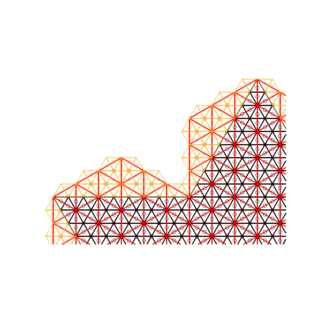

7.7 Square snowflake
Finally, we consider the square snowflake and the associated sequence of non-nested prefractals described in §6.5. We choose and . Plots of the resulting near- and far-field solutions for prefractal level are shown in Figure 19. Proposition 6.5 implies that we have (Galerkin) BEM convergence provided as . But numerical validation of this convergence is hampered by the fact that the minimal number of DOFs required to discretise the th-level prefractal with a uniform mesh of squares is . In order to simulate higher-level prefractals more sophisticated BEM implementations are needed, e.g. using fast matrix–vector multiplications, and non-uniform or non-convex meshes. This will be considered in future work.


8 Conclusion and open problems
In this paper we have written down in §3 well-posed BVP and BIE formulations for scattering by an acoustic screen that is either fractal or has fractal boundary, refining, simplifying, and extending (in particular through application of recent results from caetano2018) the earlier results of ScreenPaper. Generalising the treatment in ScreenPaper, we have studied in §4 (using Mosco convergence for the first time in this context) the convergence of BIE solutions on a sequence of prefractals to the solution on a limiting set ; in particular we have proved in Theorem 4.1 and Proposition 4.3 new convergence results in cases where the sequence of prefractals is not monotonically convergent to , and have applied these results in §4.1 to sequences of prefractals generated by general iterated function systems.
But the crucial novelty of the paper has been the analysis and implementation of the BEM in §§5–7. In §4.1 we have obtained, to our knowledge, the first rigorous convergence analysis of a numerical method for scattering by a fractal object and the first proofs of convergence of BEM, applied on a sequence of prefractal sets , to the solution of the BIE on the limiting set , both in cases when is fractal (in particular the fixed point of an IFS of contracting similarities satisfying the standard open set condition, for example the Cantor set or dust, the Sierpinski triangle) and in cases where is an open set with fractal boundary (for example the Koch or square snowflake). We have studied these specific cases as examples of applying these new convergence results in §6, and in numerical experiments in §7.
These results are, we consider, important first steps in understanding BIEs and their solutions on sets that are fractal or have fractal boundary, and the convergence to these solutions of BEM approximations on sequences of more regular prefractals. More generally, these results and methods are applicable to the convergence analysis of Galerkin methods for BIEs (and, we anticipate, other integral equations and PDEs) posed on any rough domain that cannot be discretised exactly but first needs to be approximated by a sequence of more regular sets.
For the specific screen scattering problems that have been the focus of this paper, and for large classes of related problems, there remain many intriguing and important open questions. These include:
- 1.
What is the regularity of the BIE solution on the limiting screen , and how does this depend on the fractal dimension of or its boundary? In the case when is fractal the density results summarised in Lemma 3.13 are one step towards addressing this question.
- 2.
At what rate do BIE solutions on a prefractal sequence converge to the limiting BIE solution on ?
- 3.
If the BIE is additionally discretised by BEM, how does the convergence rate depend jointly on the prefractal level and the discretisation? (The numerical simulations in §7 provide some experimental data.)
- 4.
Extending this question, what is the optimal balance (to achieve an accurate approximation of the solution on with least work) between increasing the prefractal level and mesh refinement? For example, for the family of pre-convex meshes (42), what is the optimal choice of the parameter ?
- 5.
In the case when is a self-similar fractal (is the attractor of an IFS of contracting similarities), can efficient BEM solvers be built making use of the self-similarity?
We hope to address some of these questions in future work, together with exploring more efficient BEM implementations (e.g. using locally-refined meshes, fast iterative solvers for structured meshes), and the extension of the methods developed here to more general problems (e.g. curvilinear screens, different boundary conditions, elastic and electromagnetic waves, other PDEs).
9 Acknowledgements
We acknowledge support from EPSRC grants EP/S01375X/1 and EP/N019407/1, from GNCS–INDAM, from MIUR through the “Dipartimenti di Eccellenza” Programme (2018–2022)–Dept. of Mathematics, University of Pavia, and from PRIN for the project “NA_FROM-PDEs”. The last author acknowledges funding from the “Bourses de stages à l’étranger” scheme of Université Paris-Saclay, which supported a research visit to UCL in May-August 2018. The authors are grateful to M. Berry, A. Buffa, A. Caetano, R. Capitanelli, R. Hiptmair, M. R. Lancia, U. Mosco, M. Negri, G. Savaré, C. Schwab, E. Spence and M. A. Vivaldi for instructive discussions.
Appendix A Finite element approximation by piecewise constants
Let and be a non-empty bounded open set. Let us say that is a pre-convex mesh on if, for some , is a collection of open subsets such that: (i) the convex hulls are pairwise disjoint; (ii) each has zero -dimensional Lebesgue measure; and (iii) . We note that (ii) holds (and this will be the case in the applications that we make) if each is the union of a finite number of pairwise disjoint Lipschitz open sets, in particular if each is convex, in which case we term a convex mesh.
In the case that is a curvilinear Lipschitz polygon and each is a curvilinear triangle or quadrilateral, the following lemma is a standard BEM error estimate (e.g. (Steinbach, Thm. 10.4, (10.10))), except that in the standard versions the explicit constant in (44) is replaced by an unknown constant that depends (in an unspecified way) on the domain and the shape regularity of the elements. The version we prove here, which applies to any bounded open set and any pre-convex mesh , and provides explicit constants independent of the domain and element shape, should be of some independent interest and is essential for our application to BEM on sequences of prefractals converging to a fractal limit.
Lemma A.1.
Let and , and let be a non-empty bounded open set and be a pre-convex mesh on . Let denote the set of piecewise constant functions on , so that if and is constant, for . Let be orthogonal projection, so that
Let . Then, for and , if , then
| (44) |
where on the left hand side we extend from to by zero to become an element of .
Proof.
Clearly (44) holds for as , with identical norms, and is an orthogonal projection operator on . Now suppose that and . In this case, recalling that with equal norms, and that , the required bound (44) is implied by
| (45) |
where is such that and . To see that this bound holds, let denote the convex hull of , for , which has the same diameter as , and let , so that is a convex mesh on . Let denote the space of piecewise constant functions on , be orthogonal projection, and . Then so that
But
for some , by the standard Poincaré inequality. Indeed, since is convex, this bound holds with , where , which is known Bebendorf03; PayneWeinberger60 to be the best constant in this inequality for convex domains. The inequality (45) follows since the are pairwise disjoint.
Thus (44) is proved for and , and by interpolation it extends to and . Precisely, let denote the norm on the -method interpolation space , with the normalisation defined in (InterpolationCWHM, (7,8)). Then
| (46) |
where the first inequality follows by interpolation since with equality of norms given the normalisation (InterpolationCWHM, (7,8)) (see (InterpolationCWHM, Lem. 2.1(iii), Thm. 2.2(i))); the second inequality holds since, again given this normalisation, the embedding of into has norm (InterpolationCWHM, Lem. 4.2).
Finally, suppose that and . Then, as is a unitary realisation of the dual space of via an extension of the inner product, if then
where the final bound follows from the Cauchy–Schwarz inequality and two applications of (46). ∎
Appendix B Mollification and Sobolev regularity
Given , choose with for and , and for let
Given , for and we define , the -mollification of , by , where
in the case that , and, in the case that , the definition of is extended to all by continuity and density. It is standard that in as (e.g. (McLean, Exercise 3.17)). Moreover, with the Fourier transform normalised as in §2.4, we have that
where . Hence it holds for that
where
Since , it holds for that
for . Thus, for , , and , it holds that
| (47) |
References
- (1) Y. Achdou, C. Sabot, and N. Tchou, Transparent boundary conditions for the Helmholtz equation in some ramified domains with a fractal boundary, J. Comput. Phys., 220 (2007), pp. 712–739.
- (2) E. A. Algehyne and A. J. Mulholland, A finite element approach to modelling fractal ultrasonic transducers, IMA J. Appl. Math., 80 (2015), pp. 1684–1702.
- (3) E. A. Algehyne and A. J. Mulholland, Analysis of a fractal ultrasonic transducer with a range of piezoelectric length scales, IMA J. Appl. Math., 84 (2019), pp. 605–631.
- (4) K. Arfi and A. Rozanova-Pierrat, Dirichlet-to-Neumann or Poincaré-Steklov operator on fractals described by -sets, Discret. Contin. Dyn. S., 12 (2019), pp. 1–26.
- (5) J. M. Arrieta and P. D. Lamberti, Higher order elliptic operators on variable domains. stability results and boundary oscillations for intermediate problems, J. Differential Equations, 263 (2017), pp. 4222–4266.
- (6) P. Bagnerini, A. Buffa, and E. Vacca, Mesh generation and numerical analysis of a Galerkin method for highly conductive prefractal layers, Appl. Numer. Math., 65 (2013), pp. 63–78.
- (7) L. Banjai and L. Boulton, The Poincaré constant of the Koch snowflake, arxiv:1708.08401, (2017).
- (8) J. Bannister, A. Gibbs, and D. P. Hewett, Acoustic scattering by impedance screens/cracks with fractal boundary: well-posedness analysis and boundary element approximation, arxiv:2009.13236, (2020).
- (9) A. J. Baran, A review of the light scattering properties of cirrus, J. Quant. Spectrosc. Ra., 110 (2009), pp. 1239–1260.
- (10) M. Bebendorf, A note on the Poincaré inequality for convex domains, Z. Anal. Anwend., 22 (2003), pp. 751–756.
- (11) F. Ben Hassen, Y. Boukari, and H. Haddar, Application of the linear sampling method to identify cracks with impedance boundary conditions, Inverse Probl. Sci. En., 21 (2013), pp. 210–234.
- (12) M. V. Berry, Diffractals, J. Phys. A: Math. Gen., 12 (1979), p. 781.
- (13) A. Bespalov, N. Heuer, and R. Hiptmair, Convergence of the natural hp-BEM for the electric field integral equation on polyhedral surfaces, SIAM J. Numer. Anal., 48 (2010), pp. 1518–1529.
- (14) C. J. Bouwkamp, Diffraction theory, Rep. Prog. Phys., 17 (1954), pp. 35–100.
- (15) D. Bucur and N. Varchon, Boundary variation for a Neumann problem, Ann. Scuola Norm. Sup. Pisa Cl. Sci. (4), 29 (2000), pp. 807–821.
- (16) A. Buffa and S. H. Christiansen, The electric field integral equation on Lipschitz screens: definitions and numerical approximation, Numer. Math., 94 (2003), pp. 229–267.
- (17) A. Caetano, D. P. Hewett, and A. Moiola, Density results for Sobolev, Besov and Triebel-Lizorkin spaces on rough sets, arxiv:1904.05420, (2018).
- (18) R. Capitanelli and M. Vivaldi, FEM for quasilinear obstacle problems in bad domains, ESAIM: Math. Model. Num., 51 (2017), pp. 2465–2485.
- (19) R. Capitanelli and M. A. Vivaldi, Weighted estimates on fractal domains, Mathematika, 61 (2015), pp. 370–384.
- (20) M. Cefalo, M. Lancia, and H. Liang, Heat-flow problems across fractal mixtures: regularity results of the solutions and numerical approximation, Differ. Integral Equ., 26 (2013), pp. 1027–1054.
- (21) M. Cefalo and M. R. Lancia, An optimal mesh generation algorithm for domains with Koch type boundaries, Math. Comput. Simulat., 106 (2014), pp. 133–162.
- (22) R. Ceolato, M. J. Berg, and N. Riviere, Spectral and angular light-scattering from silica fractal aggregates, J. Quant. Spectrosc. Ra., 131 (2013), pp. 160–165.
- (23) S. Chandler-Wilde and M. Lindner, Coburn’s lemma and the finite section method for random Jacobi operators, J. Funct. Anal., 270 (2016), pp. 802–841.
- (24) S. N. Chandler-Wilde, Convergence of boundary element methods on fractals, in Boundary Elements Methods, Mathematisches Forschungsinstitut Oberwolfach Report No. 5/2020, S. Chaillat-Loseille, R. Hiptmair, and O. Steinbach, eds., 2020, pp. 26–30.
- (25) S. N. Chandler-Wilde and D. P. Hewett, Wavenumber-explicit continuity and coercivity estimates in acoustic scattering by planar screens, Integr. Equat. Oper. Th., 82 (2015), pp. 423–449.
- (26) S. N. Chandler-Wilde and D. P. Hewett, BVP and BIE formulations for scattering by fractal screens, in Proc. 13th Int. Conf. on Mathematical and Numerical Aspects of Wave Propagation, Minneapolis, USA, 2017, pp. 85–90.
- (27) S. N. Chandler-Wilde and D. P. Hewett, Well-posed PDE and integral equation formulations for scattering by fractal screens, SIAM J. Math. Anal., 50 (2018), pp. 677–717.
- (28) S. N. Chandler-Wilde, D. P. Hewett, and A. Moiola, Interpolation of Hilbert and Sobolev spaces: quantitative estimates and counterexamples, Mathematika, 61 (2015), pp. 414–443.
- (29) S. N. Chandler-Wilde, D. P. Hewett, and A. Moiola, Sobolev spaces on non-Lipschitz subsets of with application to boundary integral equations on fractal screens, Integr. Equat. Operat. Th., 87 (2017), pp. 179–224.
- (30) J. M. Christian, G. S. McDonald, A. Kotsampaseris, and J. Huang, Fresnel diffraction patterns from fractal apertures: boundary conditions and circulation, pentaflakes and islands, in Proceedings of EOSAM 2016, Berlin, Germany, European Optical Society, 2016.
- (31) X. Claeys and R. Hiptmair, Integral equations on multi-screens, Integr. Equat. Oper. Th., 77 (2013), pp. 167–197.
- (32) D. Colton and R. Kress, Inverse Acoustic and Electromagnetic Scattering Theory, Springer, 2nd ed., 1998.
- (33) J. B. Conway, A Course in Functional Analysis, Springer, 2nd ed., 1990.
- (34) D. Daners, Dirichlet problems on varying domains, J. Differential Equations, 188 (2003), pp. 591–624.
- (35) M. Durand, Layer potentials and boundary value problems for the Helmholtz equation in the complement of a thin obstacle, Math. Meth. Appl. Sci., 5 (1983), pp. 389–421.
- (36) E. Evans, A finite element approach to extension using prefractals, Adv. Math. Sci. Appl, 22 (2012), pp. 391–420.
- (37) K. Falconer, Fractal Geometry: Mathematical Foundations and Applications, Wiley, 3rd ed., 2014.
- (38) H. Fang, Z. Qiu, A. Mulholland, R. O’Leary, and A. Gachagan, Broadband 1-3 piezoelectric composite transducer design using Sierpinski gasket fractal geometry, IEEE T. Ultrason. Ferr., 65 (2018), pp. 2429–2439.
- (39) B. Ghosh, S. N. Sinha, and M. V. Kartikeyan, Fractal Apertures in Waveguides, Conducting Screens and Cavities, Springer, 2014.
- (40) D. S. Grebenkov and B.-T. Nguyen, Geometrical structure of Laplacian eigenfunctions, SIAM Review, 55 (2013), pp. 601–667.
- (41) P. Grisvard, Elliptic Problems in Nonsmooth Domains, Pitman, 1985.
- (42) T. Ha-Duong, On the transient acoustic scattering by a flat object, Japan J. Indust. Appl. Math., 7 (1990), pp. 489–513.
- (43) D. P. Hewett and J. Bannister, Acoustic scattering by impedance screens with fractal boundary, in Proc. 14th Int. Conf. on Mathematical and Numerical Aspects of Wave Propagation, Vienna, Austria, 2019, pp. 80–81.
- (44) D. P. Hewett, S. Langdon, and S. N. Chandler-Wilde, A frequency-independent boundary element method for scattering by two-dimensional screens and apertures, IMA J. Numer. Anal., 35 (2015), pp. 1698–1728.
- (45) D. P. Hewett and A. Moiola, On the maximal Sobolev regularity of distributions supported by subsets of Euclidean space, Anal. Appl., 15 (2017), pp. 731–770.
- (46) H. Holm, M. Maischak, and E. P. Stephan, The hp-version of the boundary element method for Helmholtz screen problems, Computing, 57 (1996), pp. 105–134.
- (47) P. Horváth, P. Šmíd, I. Vašková, and M. Hrabovskỳ, Koch fractals in physical optics and their Fraunhofer diffraction patterns, Optik, 121 (2010), pp. 206–213.
- (48) C. Hua and B. Sleeman, High-frequency estimates for the Neumann scattering phase in non-smooth obstacle scattering, Inverse Probl., 17 (2001), p. 1.
- (49) F. Ihlenburg, Finite Element Analysis of Acoustic Scattering, Springer, 1998.
- (50) A. D. Jaggard and D. L. Jaggard, Cantor ring diffractals, Opt. Commun., 158 (1998), pp. 141–148.
- (51) P. Joly and A. Semin, Mathematical and numerical modeling of wave propagation in fractal trees, C. R. Acad. Sci. I-Math., 349 (2011), pp. 1047–1051.
- (52) P. Jones, J. Ma, and V. Rokhlin, A fast direct algorithm for the solution of the Laplace equation on regions with fractal boundaries, J. Comput. Phys., 113 (1994), pp. 35–51.
- (53) T. Kato, Perturbation Theory for Linear Operators, Springer, corrected printing of 2nd ed., 1995.
- (54) R. Kress and K.-M. Lee, Integral equation methods for scattering from an impedance crack, J. Comput. Appl. Math., 161 (2003), pp. 161–177.
- (55) M. R. Lancia, M. Cefalo, and G. Dell’Acqua, Numerical approximation of transmission problems across Koch-type highly conductive layers, Appl. Math. Comput., 218 (2012), pp. 5453–5473.
- (56) W. McLean, Strongly Elliptic Systems and Boundary Integral Equations, CUP, 2000.
- (57) G. Menegatti and L. Rondi, Stability for the acoustic scattering problem for sound-hard scatterers, Inverse Probl. Imaging, 7 (2013), pp. 1307–1329.
- (58) U. Mosco, Convergence of convex sets and of solutions of variational inequalities, Advances in Mathematics, 3 (1969), pp. 510–585.
- (59) U. Mosco, An introduction to the approximate solution of variational inequalities, in Constructive Aspects of Functional Analysis, G. Geymonat, ed., C.I.M.E., Ed. Cremonese, Roma, 1971, pp. 497–682.
- (60) U. Mosco, Analysis and numerics of some fractal boundary value problems, in Analysis and Numerics of Partial Differential Equations, F. Brezzi, P. Colli Franzone, U. Gianazza, and G. Gilardi, eds., Springer, 2013, pp. 237–255.
- (61) A. J. Mulholland and A. J. Walker, Piezoelectric ultrasonic transducers with fractal geometry, Fractals, 19 (2011), pp. 469–479.
- (62) J. M. Neuberger, N. Sieben, and J. W. Swift, Computing eigenfunctions on the Koch snowflake: A new grid and symmetry, J. Comput. Appl. Math., 191 (2006), pp. 126–142.
- (63) P. Panagiotopoulos and O. Panagouli, The BEM in plates with boundaries of fractal geometry, Eng. Anal. Bound. Elem., 17 (1996), pp. 153–160.
- (64) L. E. Payne and H. F. Weinberger, An optimal Poincaré inequality for convex domains, Arch. Rational Mech. Anal., 5 (1960), pp. 286–292.
- (65) C. Puente-Baliarda, J. Romeu, R. Pous, and A. Cardama, On the behavior of the Sierpinski multiband fractal antenna, IEEE T. Antenn. Propag., 46 (1998), pp. 517–524.
- (66) A. Quarteroni, R. Sacco, and F. Saleri, Numerical mathematics, Springer, 2nd ed., 2007.
- (67) W. Rudin, Functional Analysis, McGraw-Hill, 2nd ed., 1991.
- (68) B. Sapoval, T. Gobron, and A. Margolina, Vibrations of fractal drums, Phys. Rev. Lett., 67 (1991), p. 2974.
- (69) S. A. Sauter and C. Schwab, Boundary Element Methods, Springer, 2011.
- (70) B. Sleeman and C. Hua, An analogue of Berry’s conjecture for the phase in fractal obstacle scattering, IMA J. Appl. Math., 49 (1992), pp. 193–202.
- (71) W. Śmigaj, T. Betcke, S. Arridge, J. Phillips, and M. Schweiger, Solving boundary integral problems with BEM++, ACM Trans. Math. Software, 41 (2015), pp. Art. 6, 40.
- (72) T. H. M. Stein, C. D. Westbrook, and J. C. Nicol, Fractal geometry of aggregate snowflakes revealed by triple-wavelength radar measurements, Geophys. Res. Lett., 42 (2015), pp. 176–183.
- (73) O. Steinbach, Numerical Approximation Methods for Elliptic Boundary Value Problems, Springer, 2008.
- (74) E. P. Stephan, Boundary integral equations for screen problems in , Integr. Equat. Oper. Th., 10 (1987), pp. 236–257.
- (75) E. P. Stephan and W. L. Wendland, An augmented Galerkin procedure for the boundary integral method applied to two-dimensional screen and crack problems, Appl. Anal., 18 (1984), pp. 183–219.
- (76) H. Triebel, Fractals and Spectra, Birkhäuser, 1997.
- (77) H. Triebel, Function spaces and wavelets on domains, EMS, 2008.
- (78) J. Tyynelä, J. Leinonen, D. Moisseev, and T. Nousiainen, Radar backscattering from snowflakes: Comparison of fractal, aggregate, and soft spheroid models, J. Atmos. Ocean. Tech., 28 (2011), pp. 1365–1372.
- (79) R. Verma, M. K. Sharma, V. Banerjee, and P. Senthilkumaran, Robustness of Cantor diffractals, Opt. Express, 21 (2013), pp. 7951–7956.
- (80) W. L. Wendland and E. P. Stephan, A hypersingular boundary integral method for two-dimensional screen and crack problems, Arch. Rational Mech. Anal., 112 (1990), pp. 363–390.
- (81) D. H. Werner and S. Ganguly, An overview of fractal antenna engineering research, IEEE Antenn. Propag. M., 45 (2003), pp. 38–57.