Regularized Estimation and Feature Selection in Mixtures of Gaussian-Gated Experts Models
Abstract
Mixtures-of-Experts models and their maximum likelihood estimation (MLE) via the EM algorithm have been thoroughly studied in the statistics and machine learning literature. They are subject of a growing investigation in the context of modeling with high-dimensional predictors with regularized MLE. We examine MoE with Gaussian gating network, for clustering and regression, and propose an -regularized MLE to encourage sparse models and deal with the high-dimensional setting. We develop an EM-Lasso algorithm to perform parameter estimation and utilize a BIC-like criterion to select the model parameters, including the sparsity tuning hyperparameters. Experiments conducted on simulated data show the good performance of the proposed regularized MLE compared to the standard MLE with the EM algorithm.
Keywords:
Mixtures-of-Experts Clustering Feature selection EM algorithm Lasso High-dimensional data.1 Introduction
Mixture-of-experts (MoE), originally introduced in [12, 13], form a class of conditional mixture models [16] for modeling, clustering and prediction in the presence of heterogeneous data. Their construction rely on conditional mixture models [16] in which both the gating network, formed by the mixing proportions, and the experts network formed by the mixture components, depend on the predictors or the inputs. The most popular choices for the gating network are the softmax gating functions [12] or the Gaussian gating functions; the latter is a particular case of the exponential family gating functions introduced in [24].
Different choices are now common for the expert network model, depending on the type of the observed responses. For instance, a model for normal observations for regression and clustering was introduced in [5] or non-normally distributed expert models like in [1] to deal with skewed data distributions [3], to ensure robustness to outliers [2, 19], or to accommodate both skewness and robustness as in [4]. A detailed review on MoE models can be found in [17]
Fitting MoE is generally performed by maximum-likelihood estimation (MLE) via the EM algorithm or its variants [8, 15]. In a high-dimensional setting, the regularization of the MLE, to perform parameter estimation under a sparsity hypothesis and hence to simultaneously perform feature selection, has been studied in [14] and more recently in [7, 11]. These approaches consider and penalties for the log-likelihood function, and are constructed upon softmax gating functions.
In this paper, we consider MoE with Gaussian gated functions, and propose an -regularized MLE via and EM-Lasso algorithm. We study the performance of the proposal on an experimental setup. The remainder of this paper is organized as follows. Section 2 describes the MoE modeling framework, and the Gaussian-gated MoE and its MLE with the EM algorithm. Then, Section 3 presents the proposed regularized MLE and the EM-Lasso algorithm. Finally, Section 4 is dedicated to numerical experiments.
2 Gaussian-Gated Mixture-of-Experts
2.1 MoE modeling framework
We consider mixtures-of-experts model to relate a high-dimensional predictor to a response , potentially multivariate . We assume that the pair is generated from a heterogeneous population governed by a hidden structure represented by a latent categorical variable . Assume that we observe a random sample of independently and identically distributed (i.i.d) pairs from , and let be an observed data sample. Assume that the pair follows a MoE distribution, then the MoE model can be defined as
| (1) |
where is the distribution of the hidden variable given the predictor with parameters , which represents the gating network, and the conditional component densities represent the experts network whose parameters are .
2.2 Gaussian-Gated Mixture-of-Experts
Let us define by the probability density function of a Gaussian random vector of dimension with mean and covariance matrix . We consider mixture-of-experts for clustering and regression of heterogeneous data. In this case, the mixture of Gaussian-gated experts models, we abbreviate as MoGGE, for multivariate real responses, is defined by (1) where the experts are (multivariate) Gaussian regressions, given by
| (2) |
and the gating network is defined by Gaussian gating function of the form:
| (3) |
with , (). This Gaussian gating network was introduced in [24] to sidestep the need for a nonlinear optimization routine in the inner loop of the EM algorithm in the case of a softmax function for the gating network. The MoGGE model is thus parameterized by the parameter vector where is the parameter vector of the gating network and is the parameter vector of experts network, with and for . The approximation capabilities of this model have been studied very recently in [18].
2.3 Maximum likelihood estimation via the EM algorithm
Mixtures-of-experts of the form (1) with softmax gating functions are in general estimated by maximizing the (conditional) log-likelihood by using the EM algorithm , in which the M-step requires an internal iterative numerical optimization procedure (eg. a Newton-Raphson algorithm) to update the softmax parameters. We follow the approach of estimating MoGGE in [24], which relies on maximizing the joint loglikelihood, and in the MLE, the M-Step can then be solved in a closed form. Indeed, based on equations (1), (2), and (3), we the MoGGE conditional density is given by:
| (4) |
Then we can write the joint density as:
| (5) | |||||
The joint log-likelihood to be maximized by EM is therefore given by:
| (6) |
2.4 The EM algorithm for the MoGGE model
The complete-data log-likelihood upon which the EM principle is constructed is then defined by
| (7) |
where being an indicator binary-valued variable such that if (i.e., if the th pair is generated from the th expert and otherwise. The EM algorithm, after starting with an initial solution , alternates between the E- and the M- Steps until convergence (when there is no longer a significant change in the log-likelihood (6)).
E-step:
Compute the expectation of the complete-data log-likelihood (7), given the observed data and the current parameter vector estimate :
| (8) | |||||
where:
| (9) |
is the posterior probability that the observed pair is generated by the th expert. This step therefore only requires the computation of the posterior component membership probabilities , for .
M-step:
Updating the the gating networks’ parameters:
Updating the experts’ network parameters
Maximizing (12) w.r.t ’s corresponds to the M-Step of standard MoE with multivariate Gaussian regression experts, see e.g [6]. The closed-form updating formulas are given by:
| (16) | |||||
| (17) | |||||
| (18) |
However, in a high dimensional setting, MLE may be unstable or even unfeasible. One possible way to proceed in such a context is the regularization of the objective function. In the context of MoE models, this has been studied namely in [14, 7, 11] where and regularization for the log-likelihood function of the standard MoE model with softmax gating network. This penalized MLE allow an efficient estimation for simultaneous parameter estimation and feature selection.
3 Penalized maximum likelihood parameter estimation
Here we study the regularized estimation of the MoGGE model. We first consider the case when (univariate response ). The expert densities are thus defined by with .
In our proposed approach, rather than maximizing the joint log-likelihood (6), we attempt to maximize its -regularized version, to encourage sparse models and to perform estimation and feature selection. The resulting penalized log-likelihood can then be defined by:
| (19) |
where is the observed-data log-likelihood of defined by (6) and is a Lasso [22] regularization term encouraging sparsity for the expert network parameters and the gating network parameters, with and positive real values representing tuning hyperparameters. For regularizing the expert parameters, the penalty is naturally applied to the regression coefficient vectors . For the gating network, since the estimates are those of a Gaussian mixture, we then follow the strategy of feature selection in model-based clustering in [20] in which we apply the penalty to the Gaussian mean vectors and assume that the Gaussian covariance matrices of the gating network are diagonal, ie. . The penalty function is then given by:
| (20) |
We now derive an EM-Lasso algorithm to maximize (19).
3.1 The EM-Lasso algorithm for the MoGGE model
Lets first define the penalized joint complete-data log-likelihood, which is given by
| (21) |
where is the non-regularized joint complete-data log-likelihood defined by (7). The EM-Lasso algorithm then alternates between the two following steps until convergence (when there is no significant change in (19).
E-step.
M-step.
This step updates the value of the parameter vector by maximizing the -function (8) with respect to , that is, by computing the parameter vector update Now we have this decomposition
| (23) |
and the maximization is performed by separate maximizations of the penalized -functions and .
Coordinate Ascent for updating the gating network
Updating the gating network parameters consists of maximizing w.r.t the following penalized -function
It can be seen that the updates of the ’s are unchanged compared to the standard algorithm and are given by (13). For the mean vectors, updating the coefficients corresponds to weighted version or and -regularized maximum likelihood estimation a Gaussian mean; The coefficients can then be updated in a cyclic way by using a Coordinate ascent algorithm until (3.1) is maximized. Coordinate ascent (CA) [10, sec. 5.4] [9, 23] is indeed an efficient way to solve Lasso-regularization problems. For each coefficient index , it can be easily shown that, after starting with the previous EM-Lasso estimate as initial value, i.e, , each iteration of the CA algorithm updates are given by the following updating formulas (see eg. [20]), written in a scalar and a vector form:
| (24) | |||||
with, is the usual non-regularized MLE update for (Eq. (14)), the th column of , is a vector of ones of size , , and is the soft-thresholding operator with . The CA procedure is iterated until no significant change in (3.1) is observed. We then take the update at convergence of the CA algorithm, i.e . Finally, the updates of the diagonal elements of the co-variance matrices are given by:
| (25) |
Coordinate Ascent for updating the experts network
The maximization step for updating the expert parameters consists of maximizing the function given by:
Updating , for each component , consists of solving an independent weighted Lasso problem where the weights are the posterior component membership probabilities . Each of these weighted Lasso problems is then separately solved by Coordinate Ascent. The CA algorithm, after starting from the previous EM-Lasso estimate as initial values, i.e , calculates, at each iteration , the following coordinate updates, until no significant change in (3.1):
| (26) | |||||
| (27) |
with , is the residual without considering the contribution of the -th coefficient, and . The parameter vector update is then taken at convergence of the CA algorithm, i.e . Then, the intercept and the variance, have the following standard updates:
| (28) | |||||
| (29) | |||||
| (30) |
3.2 Algorithm tuning and model selection
In practice, appropriate values of the tuning parameters as well as the number of experts should be chosen. In order to select them, we use a modified BIC based on a grid of candidate values for , and . This modified BIC is an extension of the criterion used in [21] for regularized mixture of regressions and was used in [7, 11] and is defined as:
| (31) |
where is the penalized log-likelihood estimator obtained by the EM-Lasso algorithm, and is the estimated number of non-zero coefficients in the model, interpreted as the degrees of freedom. Let’s assume that , whith the true number of expert components. For each value of , we define grids of tuning parameters and . For each triplet , we calculated the penalized log-likelihood estimators and compute . Finally, the model with parameters having the highest BIC value, is then selected.
4 Experimental study
In this section, we study the performance of our approach on simulated data. The codes are written in Matlab and in R and will be made publicly available on https://github.com/fchamroukhi. Different evaluation criteria are used to assess the model’s performance, including sparsity, estimation of parameters and clustering accuracy.
Sparsity performance
In order to evaluate the sparsity of the model, we calculate the specificity/sensitivity defined by:
- •
Sensitivity: proportion of correctly estimated zero coefficients;
- •
Specificity: proportion of correctly estimated nonzero coefficients.
Clustering performance
For measuring the clustering performance, we calculate the correct classification rate and the Adjusted Rate index (ARI) between the true simulated partition and the partition estimated by the EM algorithms. The estimated cluster labels are obtained by plugin the Baye’s allocation rule for the estimated model, which consists of maximizing the posterior probabilities defined in 9 and calculated with the estimated parameters. That is, the estimated class label for the -th pair is given by
| (32) |
For calculating the classification rate, we evaluate all the possible permutations of the obtained partition, and the one giving the best rate is then retained.
4.1 Simulation study
The data are generated according to the following generative hierarchical process:
We consider a MoGGE model of expert components. The parameters of the Gaussian gating function, whose prior probabilities are , are , and with . The parameters of the Gaussian expert regressors are , , and . For each data set, we sample data pairs, and for each experiment, datasets were generated to average the results and provide error bars. In order to get the best model for each sample in the sense of the BIC criterion, we estimated the penalized model with the following grids of values for the parameters: , ; The minimum and maximum values selected for and are respectively , and , . Then we selected the penalized model which maximizes the modified BIC value (31). The results will be provided in the parts below.
Obtained results
Parameter estimation accuracy
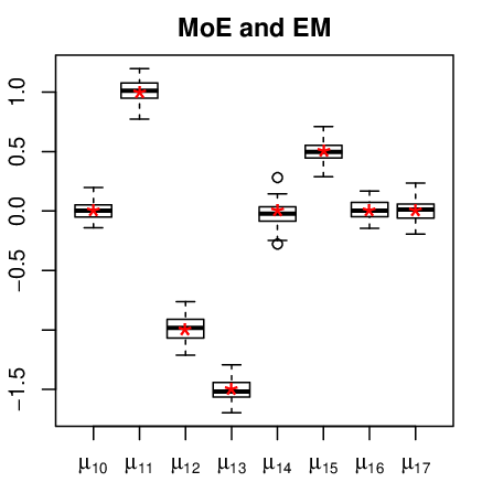
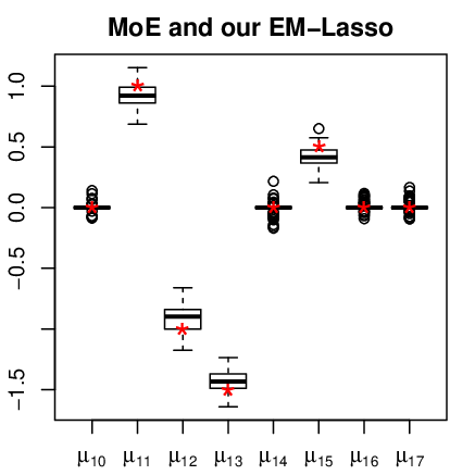
Figure 1 shows the estimated parameters for the gating network, with the error bars, for the proposed approach and for the standard MoGGE model.
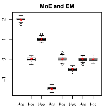
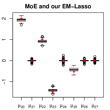
Similarly, Figure 2 shows the estimated parameters of the gating network.
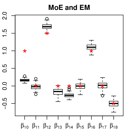
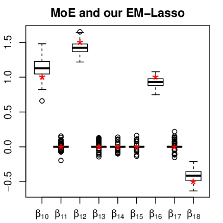
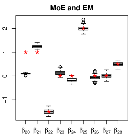
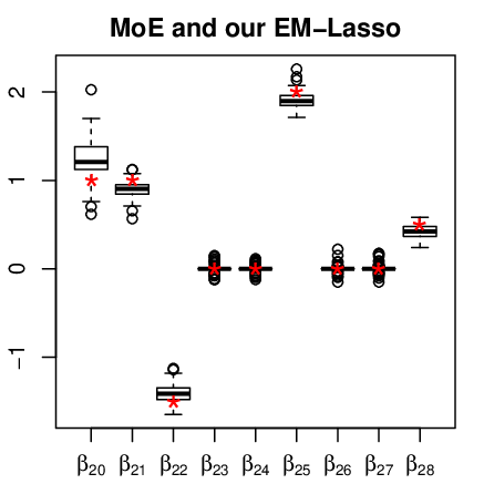
It can be seen on the two figures that, as expected, the proposed lasso-regularization approach with the proposed EM-Lasso algorithm, clearly provides models that are sparser, compared to the standard approach with EM, where the zero-coefficients are not precisely recovered. This is observed for both the gating function parameters, and the expert function parameters. While the penalized version we can see that it may be subject of a bias in estimating the non-zero coefficients, the parameter estimated and the bias are still reasonable. Hence, if one would to encourage sparsity, and to still have a good performance in density estimation, then the penalized MoGGE is a better choice, compared to the standard MLE of the MoGGE model.
Sensitivity/specificity results
Table 1 gives the sensitivity (S1) and specificity (S2) results for the two compared approaches.
| Method | Expert 1 | Expert 2 | Gate | |||
|---|---|---|---|---|---|---|
| S1 | S2 | S1 | S2 | S1 | S2 | |
| MoGGE-EM | 0.000 | 1.000 | 0.000 | 1.000 | 0.000 | 1.000 |
| MoGGE-EMLasso-BIC | 0.790 | 1.000 | 0.785 | 1.000 | 0.779 | 1.000 |
Note that here since we have two components, then only the estimation of one Gaussian gating function is considered, as the parameters of the other one are zeros. It can be seen that, none of the parameters in the non penalized model has a null value. The penalized model provides naturally sparser models compared to the standard non-penalized one.
Clustering results
We calculate the accuracy of clustering for each data set. The results in terms of correct classification rate and ARI values are provided in Table 2. We can see that the classification rate as well as as the Adjusted Rand Index are very close for the two methods, with a slight advantage to the proposed approach.
| Model | C.rate | ARI |
|---|---|---|
| MoGGE - EM | 97.25%(0.8770%) | 89.28%(3.325%) |
| MoGGE-EMLasso-BIC | 97.43%(0.8521%) | 89.99%(3.231%) |
Selecting the sparsity tuning parameters
We compute the Lasso path for a sample with same parameters as presented at the beginning of the section. On Figure 3, we observe that even with very small values (null value as well, i.e. non penalized MoE) of , the true zero parameters have values very close to zero. We also note that for values of ratio close to 0.8 for both and , almost every true zero parameters have null values and the slight bias introduced in the true nonzero parameters is reasonable.


5 Conclusion and future work
In this paper, the mixture of Gaussian-gated experts is studied towards modeling and clustering of heterogeneous regression data with high-dimensional predictors. A regularized MLE approach is proposed to simultaneously perform parameter estimation and feature selection. The developed EM-Lasso algorithm to fit the model relies on coordinate ascent updates of the regularized parameters, and its application in numerical experiments clearly shows it provides sparse models. Its performance is also compared to the state-of-the art fitting with the EM algorithm, shows its good performance, in particular in terms of sparsity. The diagonal hypothesis of the covariance matrix to derive the regularization (19) is now being relaxed, so that the regularization is on the elements of the precision matrix, i.e a graphical Lasso regularization. A future extension will also consider multivariate response with dedicated sparsity on the matrices of regression coefficients.
Acknowledgments
This research is supported by Ethel Raybould Fellowship (Univ. of Queensland), ANR SMILES ANR-18-CE40-0014, and Région Normandie RIN AStERiCs.
References
- [1] Chamroukhi, F.: Non-normal mixtures of experts (July 2015), arXiv:1506.06707
- [2] Chamroukhi, F.: Robust mixture of experts modeling using the -distribution. Neural Networks - Elsevier 79, 20–36 (2016)
- [3] Chamroukhi, F.: Skew-normal mixture of experts. In: The International Joint Conference on Neural Networks (IJCNN). Vancouver, Canada (July 2016)
- [4] Chamroukhi, F.: Skew mixture of experts. Neurocomputing 266, 390–408 (2017)
- [5] Chamroukhi, F., Samé, A., Govaert, G., Aknin, P.: A regression model with a hidden logistic process for feature extraction from time series. In: International Joint Conference on Neural Networks (IJCNN). pp. 489–496 (2009)
- [6] Chamroukhi, F., Trabelsi, D., Mohammed, S., Oukhellou, L., Amirat, Y.: Joint segmentation of multivariate time series with hidden process regression for human activity recognition. Neurocomputing 120, 633–644 (2013)
- [7] Chamroukhi, F., Huynh, B.T.: Regularized Maximum Likelihood Estimation and Feature Selection in Mixtures-of-Experts Models. Journal de la Société Française de Statistique 160(1), 57–85 (March 2019)
- [8] Dempster, A.P., Laird, N.M., Rubin, D.B.: Maximum likelihood from incomplete data via the EM algorithm. JRSS, B 39(1), 1–38 (1977)
- [9] Friedman, J., Hastie, T., Höfling, H., Tibshirani, R.: Pathwise coordinate optimization. Tech. rep., Annals of Applied Statistics (2007)
- [10] Hastie, T., Tibshirani, R., Wainwright, M.: Statistical Learning with Sparsity: The Lasso and Generalizations. Chapman & Hall/CRC (2015)
- [11] Huynh, T., Chamroukhi, F.: Estimation and feature selection in mixtures of generalized linear experts models. arXiv:1907.06994 (July 2019)
- [12] Jacobs, R.A., Jordan, M.I., Nowlan, S.J., Hinton, G.E.: Adaptive mixtures of local experts. Neural Computation 3(1), 79–87 (1991)
- [13] Jordan, M.I., Jacobs, R.A.: Hierarchical mixtures of experts and the EM algorithm. Neural Computation 6, 181–214 (1994)
- [14] Khalili, A.: New estimation and feature selection methods in mixture-of-experts models. Canadian Journal of Statistics 38(4), 519–539 (2010)
- [15] McLachlan, G.J., Krishnan, T.: The EM algorithm and extensions. New York: Wiley, second edn. (2008)
- [16] McLachlan, G.J., Peel., D.: Finite mixture models. New York: Wiley (2000)
- [17] Nguyen, H.D., Chamroukhi, F.: Practical and theoretical aspects of mixture-of-experts modeling: An overview. WIREs: Data Mining and Knowledge Discovery pp. e1246–n/a (Feb 2018). https://doi.org/10.1002/widm.1246
- [18] Nguyen, H.D., Chamroukhi, F., Forbes, F.: Approximation results regarding the multiple-output mixture of linear experts model. Neurocomputing doi:10.1016/j.neucom.2019.08.014 (2019)
- [19] Nguyen, H.D., McLachlan, G.J.: Laplace mixture of linear experts. Computational Statistics & Data Analysis 93, 177–191 (2016)
- [20] Pan, W., Shen, X.: Penalized model-based clustering with application to variable selection. J. Mach. Learn. Res. 8, 1145–1164 (May 2007)
- [21] Städler, N., Bühlmann, P., van de Geer, S.: Rejoinder: l1-penalization for mixture regression models. TEST 19(2), 280–285 (2010)
- [22] Tibshirani, R.: Regression shrinkage and selection via the lasso. Journal of the Royal Statistical Society, Series B 58(1), 267–288 (1996)
- [23] Wu, T.T., Lange, K.: Coordinate descent algorithms for lasso penalized regression. Ann. Appl. Stat. 2(1), 224–244 (03 2008). https://doi.org/10.1214/07-AOAS147
- [24] Xu, L., Jordan, M.I., Hinton, G.E.: An alternative model for mixtures of experts. In: Tesauro, G., Touretzky, D.S., Leen, T.K. (eds.) Advances in Neural Information Processing Systems 7, pp. 633–640. MIT Press (1995)