Bayesian Model Calibration for Extrapolative Prediction via Gibbs Posteriors
Abstract
The current standard Bayesian approach to model calibration, which assigns a Gaussian process prior to the discrepancy term, often suffers from issues of unidentifiability and computational complexity and instability. When the goal is to quantify uncertainty in physical parameters for extrapolative prediction, then there is no need to perform inference on the discrepancy term. With this in mind, we introduce Gibbs posteriors as an alternative Bayesian method for model calibration, which updates the prior with a loss function connecting the data to the parameter. The target of inference is the physical parameter value which minimizes the expected loss. We propose to tune the loss scale of the Gibbs posterior to maintain nominal frequentist coverage under assumptions of the form of model discrepancy, and present a bootstrap implementation for approximating coverage rates. Our approach is highly modular, allowing an analyst to easily encode a wide variety of such assumptions. Furthermore, we provide a principled method of combining posteriors calculated from data subsets. We apply our methods to data from an experiment measuring the material properties of tantalum.
Keywords: Inverse problem; misspecified models; physical models; uncertainty quantification
1 Introduction
Model calibration is the process of learning about model inputs by coupling experimental data with computational simulation outputs, essentially solving an inverse problem for a deterministic computer model. Typically experimental data are assumed to be generated from the process:
| (1) | ||||
where are observations of the true physical process at time measured with independent errors . The parameter is an input to the physical process and is the true value of that we are trying to learn. The true physical process is approximated by deterministic physical model , and the goal is to determine the model inputs from the observations of . However, there is some systemic bias in this physical model, and so accounts for this inadequacy and is called the model discrepancy term.
Model calibration can serve two distinct purposes in computer modeling: interpolative prediction and extrapolative prediction. In interpolative prediction, the model parameters are tuned such that the model can accurately predict throughout the design space where data have been collected. In extrapolative prediction, the calibrated model results are applied to predict in a space or setting where no data have been collected and the model cannot be directly validated. Extrapolative prediction is common in many engineering applications, as the computer modeling exercise is often intended to compensate for gaps in data. Examples of extrapolative prediction include calibrating subsystem models to roll-up results into overall system predictions (Li and Mahadevan 2016), using calibration to estimate parameters with scientific meaning for use in other applications or models (Brown and Hund 2018; Brynjarsdóttir and O’Hagan 2014), and using models to predict to spaces where data cannot be collected (Ling et al. 2014).
Physical models are inherently approximations of reality and typically contain error; thus, model calibration procedures must accommodate for model discrepancy (called model misspecification in the statistics literature) to obtain valid estimates and uncertainties on calibrated input parameters. The ontological question of whether a “true” value of a model input exists in reality is debatable, because there is no ground truth in a computer simulation. Here we take the pragmatic view that a true calibration parameter exists insofar as it informs extrapolative prediction. Therefore, we refer to such calibration parameters as “physical parameters,” following Brynjarsdóttir and O’Hagan 2014.
In this paper we present a Bayesian approach to model calibration based on Gibbs posteriors. With this method, the target of inference is the physical parameter which minimizes a user-defined loss function in expectation, and we accommodate the use of prior information when available. In the remainder of this section, we preview our method as a solution to issues of identifiability and computational stability associated with the current standard Bayesian approach, and connect it with existing ideas in the literature which cast calibration as an optimization problem. In Section 2, we explain our method in detail and motivate our approach of setting the loss scale for the Gibbs posterior, of which we present an implementation in Section 3. Then, in Section 4 we give a statistically principled method for combining posteriors calculated from data subsets. Section 5 applies our methods to data from an experiment measuring the dynamic material properties of tantalum. We close with a discussion in Section 6. The online supplement contains simulation results, algorithmic details, and additional figures.
1.1 Standard Bayesian approach
Calibration is often a poorly identified problem, where multiple inputs produce equally valid solutions. Bayesian inference has been used extensively in model calibration to avoid optimization challenges under poorly identified parameters. The most common Bayesian approach comes from the seminal paper by Kennedy and O’Hagan 2001 (hereafter, KOH), whereby the model in Eq. (1) is completed by assigning priors to the unknown components:
| (2) | ||||
where denotes the covariance kernel of the Gaussian process (GP) prior for the discrepancy . This model accommodates different sources of uncertainty, including input parameter uncertainty, measurement uncertainty in the experimental data, and model-form error. This paper is primarily concerned with this latter uncertainty, model-form error.
The KOH model allows for model misspecification through incorporation of the GP prior for the discrepancy. However, it is well known that including this term to account for model discrepancy is insufficient, because and are not jointly identifiable (Loeppky et al. 2006); various configurations of the two can explain the data equally well while having similar density under the prior. The calibration parameters are only guaranteed to converge to their true physical values when there is no discrepancy, or when the discrepancy is mean 0 over and independent of . Calibration parameters should not be expected to have physical interpretations under the KOH model in the presence of model discrepancy (Arendt et al. 2012b; Brynjarsdóttir and O’Hagan 2014). The non-identifiability of the discrepancy function is similar to the problem of “spatial confounding” in the spatial statistics literature (Reich et al. 2006; Hodges and Reich 2010; Paciorek 2010), as it is generally not possible to learn a systematic, unobserved model bias from the observed data alone.
When model inputs have physical interpretations, model discrepancy must be carefully considered for valid physical parameter estimation and uncertainty quantification. For instance, Brynjarsdóttir and O’Hagan 2014 illustrate that the KOH model results in biased parameter estimates in the presence of systematic model discrepancy, and the only way to reduce this bias is to know a priori the form of the discrepancy. Challenges associated with physical parameter calibration under model misspecification are well-documented (Arendt et al. 2012b; Arendt et al. 2012a; Brynjarsdóttir and O’Hagan 2014; Arendt et al. 2016; Tuo and Wu 2016), but few solutions exist beyond the standard KOH treatment of model discrepancy. More recent work shows that KOH calibration is not -consistent and calibration parameter inferences depend on the model discrepancy prior (Tuo and Wu 2016). To address this issue, Plumlee 2017 proposes using a prior on the discrepancy that is orthogonal to the computer model gradient to produce calibration results that are consistent with the desired loss function, similar to projected kernel calibration proposed by Tuo 2017.
A common thread across all calibration methodologies is that the analyst must make assumptions about the form of the model discrepancy in order to obtain accurate calibration parameter estimates. For instance, the KOH model assumes that model discrepancy can be represented as a Gaussian process; further, inferences about calibration parameters under KOH are generally only correct when the Gaussian procss is mean 0 and independent of the model inputs. Brynjarsdóttir and O’Hagan 2014 place stronger prior information on the Gaussian process under a non-mean 0 discrepancy to improve inferences based on knowledge of the form of the discrepancy.
1.2 An alternative Bayesian approach
The goal of this paper is to introduce a Bayesian approach for accomodating model discrepancy as an alternative to KOH, namely Gibbs posteriors. With this method, we specify a prior for the calibration parameters, and provide an update for these parameters by a loss function connecting the data and the unknown parameters. The Gibbs posterior is
where is a loss function and is a scalar apportioning weight between the data and the prior, which we call the loss scale. Crucially, as explained in greater detail in Section 2, the target of inference here is different from that under the KOH model; our motivation is to quantify uncertainty in the value that minimizes the loss in expectation under the data generating process for . In this sense, the target has a well-grounded physical interpretation. This approach provides a flexible alternative modeling framework to KOH that allows the analyst to utilize prior knowledge of how the model is wrong when possible.
The Gibbs posterior framework as introduced here for application to Bayesian model calibration has several advantages: (i) the target of inference is as the minimizer of the expected loss, avoiding issues with the ontological meaning of in KOH, and (ii) we bypass issues of computational stability associated with estimating the discrepancy function in the KOH model. Further, this approach emphasizes and responds to the need for distinct treatments of calibration for extrapolative versus interpolative prediction, analogous to predictive versus explanatory modeling in statistics (Shmueli et al. 2010). For extrapolative prediction, alternatives to KOH are lacking but needed. Previous work has employed power likelihood techniques, a special case the Gibbs posterior, for calibration (Jackson et al. 2004; Mosbach et al. 2014; Brown and Hund 2018), but to our knowledge none of this work links power likelihood methods to the emerging statistics literature on Gibbs posteriors, and it remains an open question how to select the loss scale . In this paper, we generalize previously proposed Gibbs posterior techniques for the calibration setting, and give a method of tuning the choice of loss scale.
1.3 Calibration as optimization
Given that is difficult to interpret in the KOH model due to lack of consistency, a recent trend in the calibration literature is to view calibration as an optimization problem (Tuo and Wu 2015; Wong et al. 2017; Gramacy et al. 2015). The “ideal” value of the physical parameters is defined to be the minimizer of distance between the truth physical process and the observed data:
| (3) |
However, because the true physical process is unknown, Wong et al. 2017 propose the estimator minimizing the loss between the computer prediction and the observed data:
| (4) | ||||
where characterizes a weighting scheme for . The sampling distribution of this estimator is approximated with the bootstrap.
While viewing calibration as optimization, as given above, simplifies the definition of the “best estimate” of relative to KOH, this approach is not satisfactory from a Bayesian perspective. We would prefer to give a posterior distribution for conditional on the observed data, while incorporating prior information on both the discrepancy and the model parameters when possible. Our Gibbs posterior method does exactly this. We reformulate the inferential goal of the Bayesian approach as one which quantifies uncertainty on a value which minimizes an expected loss function, in contrast to the KOH model which expresses uncertainty in a set of parameters which are involved in a specified probabilistic model given in Eqs. (1) and (2).
2 Gibbs posteriors for Bayesian model calibration
When physical parameter estimation is the goal of calibration, then we have no need to make posterior inference on a discrepancy function (which only improves interpolative prediction). With this in mind, we propose a Gibbs posterior approach to calibration under model discrepancy.
We continue to assume the data generating mechanism of Eq. (1). In connection with the frequentist literature viewing model calibration as an optimization problem, our method has the inferential goal in quantifying uncertainty around an unknown parameter which minimizes the expected value of the loss function , i.e. the target is
| (5) |
with the expectation over , the true, unknown data generating process for , a combination of the unknown physical process and measurement error .
Given a prior belief distribution on for the minimizer defined in Eq. (5) and the observed data , we propose a posterior update for in the form of
| (6) |
assuming this admits a proper density, for some , called the loss scale, which controls relative weighting of the prior and the data in the update. Bissiri et al. 2016 show that Eq. (6) constitutes a “valid and coherent” update from the prior concerning , in that, for example, it follows a sequential invariance property of updating, and minimizes an additive loss measuring respective discrepancy between the posterior and prior, and the posterior and data. The update in the form of Eq. (6) is referred to in the literature as the Gibbs posterior (Zhang 2006; Jiang and Tanner 2008a; Alquier et al. 2016). We do not incorporate the discrepancy into the posterior inference scheme, though we do use prior knowledge on it to inform the choice of loss scale, as we explain in the following subsection.
A special case of the Gibbs posterior is power-likelihood methods (Miller and Dunson 2015; Grünwald et al. 2017), where the likelihood for the (presumably misspecified) probability model is scaled by some power. However, here we are more generally interested in linking the observed data and unknown parameters via a loss function. Note that (6) accommodates power-likelihood posteriors as a special case when is the negative log-likelihood, and further, the ordinary Bayesian posterior is returned when .
The choice of loss function defines the estimand, as shown in Eq. (5). To choose the loss function, we can consider prior knowledge about model discrepancy. For instance, one loss function could be the distance between the observed data and the expected value of the true process:
| (7) |
which admits an estimand similar to that in Eq. (3). When and so , this loss function is the same as that used in the frequentist estimator in Eq. (4) when using a uniform weighting scheme on the sample space .
The main benefit of using the Gibbs posterior is now we have a well-defined target of inference coming from a user-defined loss function, in contrast to the KOH approach which has a less concrete target. As we accumulate more data, we concentrate on the empirical risk minimizer, as long as this value has positive support under the prior. Also, we can avoid the computational difficulties typical in taking the KOH approach (i.e., calculating matrix inversions in the MCMC scheme necessary when using a GP prior). We now address the question of setting the loss scale .
2.1 Choosing the loss scale by calibrating credible intervals
Gibbs posteriors, in particular power-likelihood methods, have previously been applied to model calibration (Jackson et al. 2004; Mosbach et al. 2014; Brown and Hund 2018), but it remains an open question as to how the loss scale should be selected. Outside of calibration applications, there are many other suggested for approaches (Miller and Dunson 2015; Grünwald et al. 2017; Jiang and Tanner 2008b; Holmes and Walker 2017; Syring and Martin 2018; Lyddon et al. 2017). So far there has been no universally applicable approach, though it is clear that any valid approach should require assumptions of the form of the discrepancy
In ideal situations, there exists an analytic solution. As an example, if we are willing to make the strong assumption that the model discrepancy arises from a mean 0 Gaussian process over and apply asymptotic results, then we can calculate the asymptotic posterior distribution for under the Gibbs posterior (6). Brown and Hund 2018 use this approach to justify scaling the likelihood by a function of the effective sample size of the residuals. However, heavily relying on asymptotic results may not be prudent, given that many calibration problems involve sparse data and, more importantly, this approach relies on strong assumptions about the form of the model discrepancy (mean 0 Gaussian process). A primary advantage of our Gibbs posterior approach to calibration is that this framework allows for a very broad class of such assumptions.
For the calibration problem, we propose the strategy of tuning the loss scale to achieve correct nominal frequentist coverage of the Gibbs posterior under the assumptions of the discrepancy, as approximated by a bootstrap approach. In this way, our method is similar in spirit to Syring and Martin 2018 and Lyddon et al. 2017.
Given that , the data generating process for in Eq. (5), is unknown (because the model discrepancy is unknown), we may assign it a prior . This prior then propagates uncertainty onto the distribution for the minimizer via the hierarchical formulation
| (8) | ||||
We refer to (8) as the bootstrap model, since implementation generally requires sampling over the prior distribution on the data generating mechanism. Note that, in the bootstrapped model in (8), the data generating mechanism is considered a random variable, as opposed to Eq. (5) where the data generating mechanism is fixed but unknown. As a result, in the bootstrapped model, there is stochasticity in due to measurement noise and in due to unknown model discrepancy.
Lyddon et al. 2017 consider a similar approach for the case of independent observations arising from and select the for the Gibbs posterior by matching the Fisher information of the asymptotic distributions for the Gibbs posterior (6) and bootstrap model (8). However, deriving similar analytic results for the calibration problem is likely intractable and perhaps not the most pragmatic choice in our case.
Instead, we propose selecting the loss scale to retain frequentist coverage for the Gibbs posterior, following Syring and Martin 2018. We argue that coverage is a natural metric for the calibration application, since our primary interest is sufficient uncertainty quantification (UQ) for the physical parameters of interest. One reasonable definition of sufficient UQ in this sense is accurate credible interval width under our prior assumptions on the model discrepancy. Such a requirement is stemmed in the property that, for a correctly specified model credible intervals for parameters retain frequentist coverage on average across the prior11 1 Note that coverage of credible intervals is not uniform across all , or equivalently, conditional on any particular , with the exception of the special class of “matching priors” (Ghosh 2011), i.e., in general . Generally, for a model given by , , if is a ordinary posterior credible interval, it follows that
In our case, we want to ensure that the Gibbs posterior retains frequentist coverage of the target on average under the presumed prior for the data generating process. Let denote the Gibbs posterior credible interval with scale , and let the average frequentist coverage be defined as
| (9) |
This is the frequentist probability, on average across the prior, that the Gibbs posterior credible interval with loss scale contains the true under the assumed prior . We want to choose such that . Such an approach is closely related to the “calibrated Bayes” school of thought, whereby frequentist properties are used as criteria for Bayesian model evaluation (Little 2006; Box 1980; Rubin 1984; Gelman et al. 1996).
Again, finding the optimal choice of to uphold the frequentist coverage property is analytically intractable in most cases. Instead, we propose to use Monte Carlo approximations of coverage to evaluate possible choices of using a bootstrap approach. To obtain these estimates of frequentist coverage for the Gibbs posteriors, we need to specify the prior for and generate data under this prior. For this, we propose both a parametric procedure, which we describe in detail in Section 3, and a nonparametric procedure, described in the supplement.
3 Parametric bootstrap
Here we describe a parametric bootstrap implementation to approximating Eq. (9), the average frequentist coverage of the Gibbs posterior with loss scale . Note that other implementations of the parametric bootstrap may be reasonable for scale parameter selection. The online supplement describes one such approach, and presents a simulation study which verifies that this weight selection procedure ensures nominal frequentist coverage under assumptions of discrepancy form.
We assume that a loss function has been specified to link the data and parameters of interest , for example the distance. Furthermore, we assume that a prior has been specified for the parameters of interest, as well as a prior for , i.e., and are given, with . Usually there is a Gaussian process prior for the discrepancy and a Gaussian prior for the measurement error , but here we use a more general notation, allowing these prior to be governed by some arbitrary hyperparameters and , respectively. These hyperparameters may be obtained using either empirical Bayesian estimation, expert judgment, or a combination of the two. Section 3.1 gives an empirical Bayesian procedure for estimating the hyperparameters in order to approximate . We require all priors to be proper so that samples may be drawn from them. The bootstrap procedure is then described as follows:
- (i)
Create bootstrap sample data. For , draw components from the assigned priors for the unknown values,
and from these compute the bootstrap observations to mimic draws from ,
- (ii)
Given one value of , construct credible intervals for each dataset . Then the frequentist coverage is estimated by
- (iii)
Choose the loss scale such , by using a defined grid of values or by using a stochastic approximation (Syring and Martin 2018). Using this, we can form the calibrated Gibbs posterior using the experimental data to perform final inference for .
Intuitively, one can see how the prior for (either specified with expert knowledge or through empirical Bayes) informs the final choice of loss scale. If is expected to be erratic and large in magnitude, then the point estimate for each bootstrap sample will be inaccurate, and therefore the scale must be smaller (closer to 0) so that the Gibbs posterior is more diffuse to maintain the right coverage. Conversely, if is expected to be smooth and small in magnitude, then will be close to the truth , and will be tuned to be larger.
Note that the necessary prior specifications are similarly required for the standard Bayesian approach of KOH. The difference here is that the priors are used here for the purposes of tuning the choice of . Unlike under the KOH approach, here the prior is not something that is updated in the Bayesian procedure, but rather a modeling assumption which drives the final choice of , and subsequently influences inference on . In KOH, inferences are not generally as sensitive to choice of the prior, since the prior is updated in the posterior sampling scheme. Hence, using this parametric bootstrap procedure, careful selection of is required to obtain valid inference.
3.1 Empirical Bayes prior
We can derive an empirical Bayes variant of the parametric bootstrap procedure as follows. First, find the best fitting estimate and calculate the empirical discrepancy Then, obtain estimates for and (e.g., the hyperparameters for the GP discrepancy, and the residual variance) using maximum marginal likelihood on . This approach is similar to Brown and Hund 2018, who also calculate the empirical discrepancy, in their case to estimate the effective sample size of this discrepancy to determine the appropriate scale . Further, it is analogous to residual resampling in standard parametric bootstrap approaches for regression models (Efron 1979), in that we “resample” the estimated functional discrepancy in the bootstrap procedure we describe.
3.2 Toy example
To illustrate the proposed method in a simple setting, we repeat the example given in Brynjarsdóttir and O’Hagan 2014. Consider the data generating mechanism:
| (10) |
where , , and . The goal of the calibration is to estimate . To mimic model discrepancy, the authors assume the computer model approximation is
| (11) |
with unknown. We generate observations from the true data generating mechanism, and then consider 4 models for calibrating : (i) Maximum likelihood using Eq. (11), ignoring discrepancy, (ii) the KOH model, (iii) power likelihood model following Brown and Hund 2018, and (iv) Gibbs posterior model with parametric bootstrap.
Ignoring discrepancy
KOH
Now, suppose we instead fit a KOH model that allows for discrepancy:
| (12) |
We fit the model in Eq. (12) using generalized least squares (GLS) assuming a squared-exponential kernel for the correlation function. The 95% confidence interval for is (0.48, 0.58), wider than OLS, but still too narrow to encompass the true value of .
Power-likelihood with effective sample size weighting
From the GLS fit, we follow Brown and Hund 2018 and use the estimated correlation function parameters to estimate the ESS and find , i.e. the residuals are highly autocorrelated (Figure 1(b)). We now fit a Bayesian linear regression model, with the log-likelihood scaled by . We specify a disperse normal prior for and an inverse gamma prior for . Hyperparameters were selected to make these priors proper but essentially noninformative. The 95% credible interval for is (0.43, 0.70) and now brackets the true value of . The power-likelihood approach gives exceptionally wide confidence interval estimates in this case, as we essentially do not have any degrees of freedom for parameter estimation due to the high residual autocorrelation.
Gibbs posterior with bootstrap
Finally, we implement the Gibbs posterior method with the parametric bootstrap, specifying a distribution to encode prior assumptions about model discrepancy. The parametric bootstrap procedure in Section 3 allows us to incorporate known information about discrepancy into the problem. The model discrepancy gets worse as increases, and the magnitude of the discrepancy ranges between 0 and 0.43. To mimick this mechanism, we assume a prior discrepancy of 0 over the first 1/3 of the support of and a Uniform(0, 0.4) shift over the latter 2/3 of the support. Figure 1(c) illustrates how imposing this prior distribution corrects for model discrepancy.
With this specfication of , we use the loss function in Eq. (7) and resample from the hypothesized DGM, as in Eq. (1). We obtain a loss scale of , posterior median , and a 95% posterior credible interval on of (0.58, 0.70). We again bracket the true value of , as in the ESS method, but now with greater precision in the uncertainty interval. While this example is contrived, the results clearly illustrate that the parametric bootstrap can perform well with good prior information on the discrepancy function. In the absence of this information, the method would give poor inference.


4 Ensemble calibration
In some calibration problems, it may be advantageous to divide the data into subsets, calibrate on the subsets, and then combine inferences across them. We consider two primary motivations for calibrating in subsets: (i) it can be more computationally efficient, particularly when datasets are large and/or calibration parameters vary over the model space ; and (ii) when the discrepancy is non-stationary over , updating the loss separately for different subsets of will often be simpler than trying to specify a joint loss and discrepancy prior over all of . For example, in the material model calibration problem described in Section 5, material properties can be calibrated separately for each experiment and then combined over experiments to produce a global estimate. Discrepancy may differ by experiment; by estimating separately for each one, we do not have to incorporate the changing magnitude of the discrepancy into the loss function, and we can gauge how much information each experiment provides about in the presence of discrepancy.
We refer to the idea of calibrating in subsets as “ensemble calibration.” Section 2 considered choosing a single for the entire dataset. In ensemble calibration, model misspecification is considered for subsets of the data. The data are subdivided over into subsets and each subset receives its own loss scale, so the full posterior is
| (13) |
with the methods in Sections 2 and 3 used to select loss scales for the different subsets.
Directly updating the model in Eq. (13) is disadvantageous. Gunawan et al. 2017 show that directly calibrating this joint posterior of the weighted subsets results in consistent estimates of , but uncertainty in is underestimated. An alternative solution is to calibrate each subset separately and obtain a posterior for each one:
| (14) |
The posteriors can then be combined post hoc to produce an overall estimate of the calibration parameters. This approach has computational advantages, in that calibrating each subset is simpler than the joint calibration problem. Further, the ensemble calibration approach is advantageous because we get model diagnostics for free. That is, allowing to vary over could help diagnose areas of the model space where model discrepancy could substantively change the calibration parameters. Calibrating subsets separately provides information about how calibration parameter estimates vary across the input space, which informs how discrepancy impacts the calibration parameter estimates.
Ensemble calibration is closely related to distributed Bayesian analysis, where data is divided into subsamples for subset inference (Scott et al. 2016). The resulting subset posteriors are combined into a consensus posterior distribution approximating the full data posterior. Similarly, ensemble calibration entails solving the calibration problem on subsets of the data and combining the results.
4.1 Combining subset posteriors
We apply the recently developed method of Wasserstein scalable posteriors (WASP) to combine subset posteriors (Srivastava et al. 2015). WASP divides the data into subsets, finding posteriors for each subset ; then, subset posteriors are combined into a consensus posterior by calculating an approximate Wasserstein barycenter or an “average” (with respect to Wasserstein distance) of the subset posterior distributions. As long as the number of subsets is not growing too quickly with the sample size , WASP achieves almost optimal convergence to the true parameter, , and WASP produces estimates that asymptotically converge to the full data posterior, even for many models with independent and non-identically distributed observations (Srivastava et al. 2018).
Here we use the WASP framework to provide a coherent framework for combining individually calibrated experiments into a consensus posterior. For the consensus mean we use an inverse covariance-weighted average of the subset means. While the Wasserstein barycenter mean is the unweighted average of individual means, we think a covariance-weighted average is better here for two reasons. First in our framework the covariance of each experiment is not only another parameter but also a quantification of uncertainty about the parameter of interest. Second, when normal likelihoods are used, this method provides an exact consensus posterior mean Scott et al. 2016, if we factor individual loss scales. Finally, we note that computing the consensus mean in this manner has no effect on the consensus covariance computation. An iterative algorithm, described in the supplement, is used to calculate the consensus covariance matrix.
There is a question of scaling the consensus posterior. In their original paper, Srivastava et al. use the “stochastic approximation trick”; each subset likelihood is raised to the power of . This forces the consensus posterior to reflect that we have as opposed total data points. This models the covariance of parameters across all experiments; each experiment provides a noisy estimate of and information across experiments is pooled, providing greater power. Otherwise, omitting the scaling factor , we effectively model the covariance of parameters within an individual experiment, the covariance of an “average” experiment. Based on the assumptions about the discrepancy process, , we recommend scaling as follows. When discrepancy is not known or assumed to be nonzero mean, then we recommend omitting the factor rescaling. In this case, the uncertainty from individual experiment posteriors may account for bias that does not disappear as more experiments are conducted. In the case that is known or assumed to be zero mean, has finite variance, and the for each experiment are coming from a relatively small interval, we may apply the scaling . Here experiments are providing information about parameters of interest for a specific interval of values, and as the discrepancy is zero mean, we expect parameter estimates to be unbiased. If in addition is stationary, so that its variance is not shifting with , then we may apply the scaling even to experiments over different values of . Here we expect different experiments, even over different values, to provide unbiased estimates of parameters with the same scaling of uncertainty.
Combining subset posteriors using the Wasserstein metric has several advantages. The Wasserstein metric encodes geometric information about the distribution and the sample space. For example, the Wasserstein barycenter between distributions of the same location-scale family will also be in the same location-scale family. This does not hold for Euclidean barycenters of distributions in the same location-scale family. These factors make the WASP approach more flexible in the setting of ensemble calibration. There is no need to down-weight priors, as with other methods, potentially losing conjugacy. The method can also handle deviations from Gaussianity and different specifications of loss function.
We outline our algorithmic process for combining subset posteriors and give additional detail in the online supplement; for general background in this area, see Villani 2003; Villani 2006; Gouic and Loubes 2017; Agueh and Guillaume 2011; Álvarez Esteban et al. 2016.
5 Application to dynamic material properties
Dynamic material models describe how materials behave at extreme conditions of high pressures and temperatures. To calibrate these material models, we couple computational predictions of velocity over time with experimental measurements. In this application, our goal is to calibrate parameters of the tantalum equation of state, namely the bulk modulus pressure derivative based on the model form of Vinet et al. 1989.
Here we overview the structure of the problem; details are further discussed in Brown and Hund 2018. We analyze the same data here to illustrate how our method works. We have data from 9 different experimental measurements. In the experiments, a pulsed power driver delivers massive electrical currents over short time scales through an aluminum panel, resulting in a time-dependent stress wave (impulse) propagating through the tantalum samples and then through transparent lithium fluoride windows (Figure 2, left panel). The output of interest in the velocity over time at the tantalum-lithium fluoride interface (Figure 2, right panel). Inputs to the computer model predictions include the material properties of interest for calibration and other experimental uncertainties, including: uncertainty in the boundary condition, which specifies the impulse imposed on the material sample; the thicknesses of the tantalum and aluminum samples; and the initial tantalum density.

Because the same tantalum plate was used to generate samples across all experiments, the material properties and density of tantalum do not vary between experiments. Differences between the experiments occur due to different thicknesses of the tantalum samples and different boundary conditions. A single experiment produces a functional output (a velocity curve measured over time) which can be sampled at a high rate. While there is a small amount of measurement uncertainty in velocity at each time point, smoothing this curve can essentially eliminate this measurement noise at each time point, such that the experimental outputs can be considered smooth with no measurement noise.
In this application, model discrepancy arises because there is no combination of model inputs for which the computationally predicted velocity curve can exactly match the experimental measurement (Figure 3). Whether this arises due to experimental uncertainties that distort the velocity curve or due to actual computational model error does not matter here for the mathematical formulation of discrepancy. Furthermore, since the goal is quantifying uncertainty in these physical parameters for the sake of extrapolative prediction (i.e., prediction in contexts outside these experiments), our method of Gibbs posteriors for model calibration is appropriate to use here. Since we have nine different experiments, with separate functional discrepancies expected for each, it is also convenient to calibrate each one separately and combine their respective posteriors using our ensemble approach.

For the th experiment, we consider modeling the output as , where is the computational model prediction of velocity at time points with input values of the calibration parameters , and is the discrepancy between the model prediction and experimental measurement. Failing to account for model discrepancy would essentially result in the uncertainty of the calibration parameters decreasing arbitrarily with the number of points sampled from the functional output.
In the original analysis of these data, Brown and Hund 2018 apply both a standard KOH model and a power-likelihood approach to account for model discrepancy. Equivalently, we may say they implemented a Gibbs posterior with the loss function being the Gaussian negative log-likelihood,
| (15) |
Although we previously made the comment that we can effectively assume no error in the experimental measurements, the parameter is included in this loss function to quantify the scale of the discrepancy, which is also potentially useful to compare across experiments. To select the loss scales for the Gibbs posteriors , they first obtain a point estimate for the parameters giving the best fitting output to the data, and then select based on the effective sample size (ESS) of the empirical discrepancy , so that . To compute the full posterior for , they use the joint loss function, assuming independence between experiments,
| (16) |
They conclude that the Gibbs posterior generates more computationally stable results that are consistent with prior knowledge about the material properties.
Here we reanalyze the data making two changes. First, we implement the parametric bootstrap procedure of Section 3 to tune the choice of loss scales for each experiment. We use these to obtain posteriors for each experiment independently. Then, we use the WASP method of ensemble calibration in Section 4 to combine the posteriors for each experiment into one consensus posterior. For the sake of comparison, we will also calculate the WASP consensus posterior using posteriors formed using loss scales from the ESS method. We use the same loss function (15) for the Gibbs posterior, and assign the weakly informative priors and .
We use the empirical Bayes variant of the parametric bootstrap procedure, assuming that the discrepancy follows a mean-0 GP with squared exponential covariance kernel (for simplicity we drop the subscript and explain the procedure for one experiment). We first calculate the empirical discrepancy term exactly as done by Brown and Hund 2018. Then we estimate the hyperparameters for the Gaussian process using maximum marginal likelihood on to calculate an estimate of it covariance matrix .
One bootstrap dataset is calculated as follows. First, take a draw from the prior for , , and sample a bootstrap discrepancy term using . The bootstrap dataset is calculated by . We then form equal-tailed Gibbs posterior credible intervals using for a defined grid of possible loss scale values , and check whether these intervals bracket . Following this procedure for gives a Monte Carlo estimate of frequentist coverage for the Gibbs posterior with these values of . We considered 35 values of on a log-scale for each experiment, and then fit an interpolating spline to estimate coverage as a function of , with the inverse standard error as weights for fitting the spline, and use a root finding algorithm to find which gives the nominal frequentist coverage of .
Figure 4 shows the results of the parametric bootstrap procedure for choosing the Gibbs posterior loss scales for each experiment , and compares them to those calculated from the residual ESS. At times the two differ widely, suggesting that the loss scales from ESS method could result in poor frequentist metrics. In addition, the loss scales from the parametric bootstrap tend to be closer to one another than those from ESS.
Finally, Figure 5 compares the experiment-specific posteriors and the consensus posteriors resulting from the two scaling factor selection methods for the parameter of interest. Because we combine inference across distinct experiments, we scale the consensus variance by a factor of , as explained in Section 4.1. Both consensus posteriors have similar variances, likely because the scaling factors from the two methods are, on average, similar in magnitude. However, since each experiment is weighted differently between the two methods, the means are quite far apart. This difference is due to deviations in the experiment-specific posterior variances; ESS has lower posterior variance for experiments 5 and 6, which both have relatively smaller posterior means, while the parametric bootstrap has lower posterior variance for experiment 1, which has a relatively high posterior mean. This explains the difference in consensus posterior means. The online supplement gives the loss scales and subset posteriors for each experiment for both methods.
The consensus posterior distribution presented here differs from the posterior in Brown and Hund 2018 due to differences in the estimation procedure. Specifically, the consensus posterior is based on a weighted combination of experiment-specific posteriors, rather than the joint posterior distribution in Eq. (16). The point-estimate of the parameter is an inverse-variance weighted average of the experiment specific point estimates, and, from Figure 5, we can see that two experiments (experiments 5 and 6) have small variances and also result in much lower estimates of than the remaining experiments. Hence, these experiments have substantial influence over the consensus posterior.
We consider this property at once to have both strengths and drawbacks. One possible disadvantage is that our method may be sensitive to outlying sets of data. However, the ability to examine experiment-specific posteriors and identify influential sets of data, such as experiments 5 and 6, is a key advantage of the consensus posterior approach. The experiment specific posteriors for are shown in Figure 5. We can consider whether the experiment-specific estimates are consistent with scientific knowledge or appear anomalous, which informs where model discrepancy may exist within the support of the data. This information may help identify areas where the model could be improved and/or where we might place less faith in the physical parameter estimates.
6 Discussion
When computational models are used for extrapolative prediciton, there is a need to have well-defined calibration parameters and use statistical methods which make inference more robust to model misspecification. Estimating a discrepancy function is not necessary in physical parameter estimation is the primary focus. With this motivation, we have introduced Gibbs posteriors for Bayesian model calibration when the goal is physical parameter estimation for extrapolative prediction. This generalizes previous power-likelihood approaches to model calibration.
The loss scale in the Gibbs posterior can be tuned to maintain nominal frequentist coverage under assumptions of the discrepancy form, and coverage is approximated using our bootstrap procedure. This procedure shares conceptual similarities to the pre-posterior method from Arendt et al. 2016 to determine how identifiable a calibration parameter is by repeatedly sampling discrepancy functions and evaluating variability in the calibration parameters. It is also similar to the bootstrap procedure used by Wong et al. 2017 to estimate the sampling distribution of the frequentist point estimate in Eq. (4); however, the underlying goal in our case is much different, as our bootstrap procedure is designed to calibrate the width of credible intervals from the Gibbs posterior.
There are several advantages of using the Gibbs posterior for physical parameter estimation over the existing Bayesian approach. First, the target of inference is well defined by the specified loss function, so we largely avoid the typical issues of unidentifiability. Second, the sampling scheme for Gibbs posterior is more computationally stable and less expensive than that of the current standard Bayesian method, as now we do not need to calculate matrix inversions necessary when sampling the posterior for the Gaussian process discrepancy term. Finally, our approach is highly modular; it allows for various choices of loss function to define the target of inference, and provides the analyst a large degree of freedom in specifying forms of model discrepancy to inform the choice of loss scale.
Additionally, we present a method of ensemble calibration, making the case that it is often both advantageous to calibrate separately on data subsets, and then combine their respective posteriors into a consensus posterior. An implicit assumption here is independence between subsets, and this may not always be the case. For example, in our application in Section 5, the discrepancy largely depends on the experimental conditions for each data subset, and these are likely correlated. This could be handled, for example, by incorporating dependence when combining partitions. To our knowledge, how to do this remains an open question.
Because our approach is intentionally general, there is much promise for future work. We mainly focused on using the loss to define the inferential target, and so it may be of interest to find applications where other loss functions are suitable. It would also be informative to find an application where the calibrated Gibbs posterior can be directly validated against external data or known parameter values. There are other potential bootstrapping schemes for approximating frequentist coverage to be explored, and likely more efficient means for tuning the loss scale, such as an iterative method rather than a grid search.
Acknowledgments
We would like to thank Professor Peter Müller at the University of Texas at Austin for helpful discussion, and Justin Brown at Sandia National Laboratories for allowing us to use his data for the application.
This work was supported by a Sandia National Laboratories Laboratory Directed Research and Development (LDRD) grant. Sandia National Laboratories is a multimission laboratory managed and operated by National Technology and Engineering Solutions of Sandia, LLC., a wholly owned subsidiary of Honeywell International, Inc., for the U.S. Department of Energy’s National Nuclear Security Administration under contract DE-NA0003525. Approved for unlimited release, SAND2019-10771 R. This paper describes objective technical results and analysis. Any subjective views or opinions that might be expressed in the paper do not necessarily represent the views of the U.S. Department of Energy or the United States Government.
Appendix A Alternative bootstrapping techniques
A.1 Non-parametric bootstrapping
To implement the bootstrap in Section 3, a non-parametric bootstrap could also be applied for weight selection, as in Syring and Martin 2018, where resampling with replacement is used to approximate the uncertain data generating process . The key methodological question in the calibration setting is how to resample the data to accurately represent prior uncertainty associated with model discrepancy. Standard approaches, such as simply resampling observations with replacement, must be adjusted to account for the fact that observations are not independent under model discrepancy. One way to address this lack of independence is using a block bootstrap, partitioning the data into approximately independent, non-overlapping blocks and sampling the blocks with replacement (Kreiss and Paparoditis 2011). Blocks should be selected such that model discrepancy is approximately constant over the blocks.
The validity of this nonparametric method is highly dependent on our ability to partition the data into independent blocks. Selecting blocks that are too small will result in residual dependence between blocks and subsequent underestimation of uncertainty in . Choosing blocks that are too large will result in an inability to accurately approximate the sampling distribution of under uncertainty in the data generating mechanism, again resulting in underestimation of uncertainty. With prior information about where the model discrepancy may vary over , the blocks can be selected using subject matter expertise. In the absence of such knowledge, the block size can be selected based on the autocorrelation time, assuming a stationary, mean 0 discrepancy function, resulting in equally-sized blocks. If the blocks contain different numbers of observations, the analyst must adapt the bootstrap appropriately (Sherman and Cessie 1997). If the model is systematically biased such that the expected value of the model discrepancy is non-zero, inferences on will be biased unless the loss function and resampling procedure are appropriately updated using subject matter knowledge about the expected value of the discrepancy.
This procedure is very similar to the bootstrap procedure from Syring and Martin 2018, but adapted to the autocorrelated nature of the data in the model calibration problem. More efficient implementations of this algorithm are possible by searching over in an informed way. When is multivariate, a joint credible region must be constructed.
Practical implementation of the nonparametric bootstrap can be impeded by the following disadvantages: (1) the data must be partitioned into independent blocks, which may be challenging in practice; and (2) the bootstrap will be inaccurate when the number of partitions is small, but the number of partitions is determined by the nature of the model discrepancy and cannot be arbitrarily increased.
A.2 Alternative parametric bootstrap algorithm
The bootstrap procedure below more closely mimics a classic frequentist parametric bootstrap, as described in, for instance, Syring and Martin 2018. The procedure works as follows:
- (i)
Given a value of , construct credible intervals . Generate a point estimate of , denoted , from the fitted model.
- (ii)
Create bootstrap sample data. For , Draw components, then the data is
- (iii)
Construct a MAP estimate of from the model with loss scale for each bootstrap sample, denoted .
- (iv)
The frequentist coverage is estimated by
- (v)
Choose the value of for which , by using a defined grid of values or by using a stochastic approximation (Syring and Martin 2018).
Once the optimal scale is selected, we can form the calibrated Gibbs posterior using the experimental data.
A.3 Comparison with cross validation
Cross validation is a commonly used approach to selecting , and therefore we briefly discuss how cross-validation could be applied in the calibration application. Key decisions in implementing cross validation are: (1) how to partition the data, and (2) how to select cross-validation metrics for model selection:
- •
Partitioning the data. As with the nonparametric bootstrapping method (Section A.1), when constructing cross-validation subsets, correlation between observations must be considered, because calibration data are not iid observations in the presence of model discrepancy.
- •
Metrics. Cross-validation considers the predictive ability of the model outcome to the left-out test set. We again are more concerned with uncertainty quantification than predictive accuracy, so the metric for selecting should be frequentist coverage of the model output based on the posterior predictive distribution.
Challenges in implementation. Challenges in implementing cross-validation are similar to the nonparametric bootstrapping challenges (Section A.1). Specifically, an important assumption behind this cross-validation procedure is that the partitions are samples. To achieve approximate independence between the partitions, the number of selected partitions may have to be small. When is small, then the cross-validation metrics may be highly uncertain (particularly coverage). Additionally, if some subset of the calibration parameters vary over , then implementing cross validation is not straightforward. Section 5 of the main text includes such an example.
Appendix B Simulation study for parametric bootstrap
We conduct a simulation study to test whether the parametric bootstrapping weight selection procedure achieves approximately nominal frequentist coverage for a single dynamic material properties experiment.
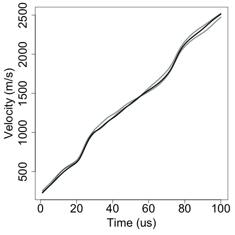
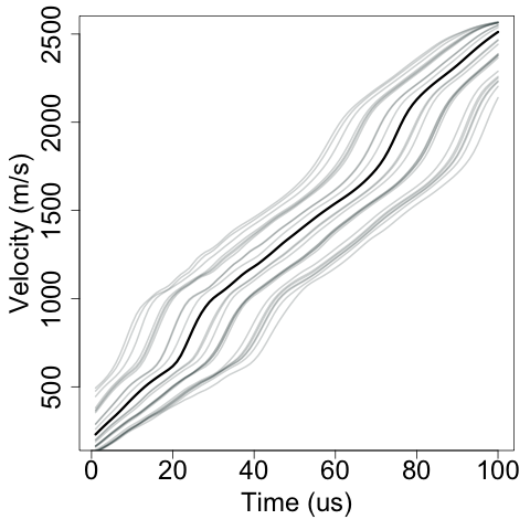
Data generating mechanism. To define the data generating model, we fix the “true” calibration parameters to their prior means for a single experiment. We assume the true model discrepancy is a mean 0 Gaussian process, with a squared exponential kernel. Example simulated datasets are shown in Figure 6, where the magnitude of the model discrepancy can be seen relative to the prior uncertainty in the calibration parameters. We use two different range parameters to determine how the shape of the discrepancy impacts the results. Specifically, the range parameter was selected such that the autocorrelation time of the Gaussian process is approximately either 1/5 or 1/10 the support of the experiment time . We refer to these settings as high versus low autocorrelation time.
Fitted model. For simplicity, we only estimate a single calibration parameter, the pressure derivative . The remaining calibration parameters are fixed to their true values. To estimate the calibration parameter and its uncertainty, we use the Gaussian negative log-likelihood as our loss function:
for . We use the same weakly informative prior on the calibration parameters as in Section 5 of the main text. A non-informative inverse gamma prior was placed on the variance parameter . A flexible generalize additive model was used to develop a computationally inexpensive surrogate model for . The accuracy of the surrogate is sufficiently high such that we anticipate that contribution of surrogate error to the simulation results will be negligible.
Methods We compare weight selection based on the parametric bootstrap to the previously proposed effective sample size method described in Brown and Hund 2018. These approaches depend on tuning parameters. Specifically, the effective sample size method depends on the estimated autocorrelation time; and the parametric bootstrap depends on the assumed form of the model discrepancy. For each method, we run the simulation study in two cases: (1) fixing the tuning parameters to their true values and (2) estimating the tuning parameters.
Using the effective sample size method, the weight was selected based on the autocorrelation time of the model discrepancy term. To estimate the autocorrleation time of the discrepancy, the computational prediction of the velocity curve at the maximum a posteriori (MAP) estimate of the calibration parameters was subtracted from the experimental data to provide a MAP estimate of the model discrepancy. The autocorrelation time was then estimated on the estimated model discrepancy using the formula described in Brown and Hund 2018.
In the parametric bootstrap, the weight was selected by assuming the model discrepancy follows a mean-zero Gaussian process (note that, given the data generating mechanism, this assumption is correct). When estimating the correlation function of the GP, we correctly assumed a Gaussian correlation functions and used a maximum likelihood estimate of the range parameter based on the estimated model discrepancy. To speed up the simulations, we used a maximum likelihood approximation to the full Bayesian model when conducting the grid search to find an optimal .
For the bootstrap models, a grid search over different weight values was implemented, using the grid of weights . The final weight was selected as the smallest weight for which the model’s 90% credible interval from the power-likelihood posterior achieved at least 90% coverage over the bootstrap resamples. To estimate coverage, we ran 100 Monte Carlo simulations (due to the computational expense of the procedure).
Results. Both the parametric bootstrap and effective sample size methods produce estimate of that are reasonably close to the true value (represented by the autocorrelation time). Further, coverage is close to the target 90% nominal coverage.
| Autocorrelation | Fixed | Estimated | |||
|---|---|---|---|---|---|
| time | E(w) | Coverage | E(w) | Coverage | |
| Parametric bootstrap | 0.1 | 0.08 | 0.95 | 0.10 | 0.92 |
| Effective sample size | 0.1 | 0.10 | 0.94 | 0.13 | 0.91 |
| Parametric bootstrap | 0.2 | 0.03 | 0.99 | 0.05 | 0.89 |
| Effective sample size | 0.2 | 0.05 | 0.93 | 0.08 | 0.86 |
Appendix C Subset posterior calculation
In this section we outline the algorithm for combining subset posteriors into a consensus posterior with WASP that was introduced in Section 4 of the main text.
When calibrating each experiment separately to obtain the constituent posteriors,
| (17) |
we must be cautious not to use the prior different times, as this would allow the prior to have undue influence on the end results. To obtain the correct prior influence for the consensus posterior using WASP, the likelihood is reweighted using a “stochastic approximation trick,” (Srivastava et al. 2015). Specifically, for subsets of equal size, each subset likelihood should be raised to the power . Essentially we are adding copies of each observation in each subset, making the implied sample size for each subset commensurate with the full data sample size.
To combine subset posteriors, we use a fixed-point algorithm for calculating quadratic Wasserstein barycenters by (Álvarez Esteban et al. 2016). The consensus location parameter is the inverse covariance-weighted average of the subset location parameters. The consensus covariance matrix is calculated by finding the covariance matrix of the barycenter for the consensus distribution’s covariance. For detailed derivation, see Álvarez Esteban et al. 2016.
The algorithm proceeds as follows.
- (1)
-
Divide data subsets, calculate each subset posterior
- (2)
-
Obtain covariance matrices and means for each subset posterior
- (3)
-
Select a starting (e.g. ), and , where is the ‘guess’ for the barycenter covariance matrix on iteration .
- (3a)
-
Calculate , defined as:
- (3b)
-
if (for some appropriate matrix norm), set and 3a, else set and continue
- (4)
-
Set
The output is location and a covariance describing the consensus posterior that is in the same location-scale family. The algorithm tends to converge very rapidly.
When all distributions being ‘averaged’ in a Wasserstein barycenter are in the same location-scale family, the algorithm converges quickly and produces an exact barycenter, also in the same location-scale family. This is well-suited to our scenario where misspecification is addressed by power likelihoods in a Gaussian setting. Raising each likelihood to a fractional power can be seen as rescaling each posterior distribution to account for misspecification and discrepancy.
The fixed-point algorithm that we use to combine subset posteriors is a more restrictive, but more accurate and cost efficient method than the full WASP procedure described in (Srivastava et al. 2015). Computationally, the full WASP procedure is implemented by first sampling subset posteriors. The approximate barycenter of these subset posterior samples is obtained through linear programming. A consensus distribution, supported on a subset of all the subset posterior points sampled, is found by minimizing the Wasserstein distance from each subset posterior to the consensus. A limiting factor for the WASP is computational feasibility; when subsets are numerous and each subset posterior has to be sampled many times, the linear program may be too costly for implementation.
An alternative popular technique for combining subset posteriors is consensus Monte Carlo (CMC). However, CMC has several properties that make it less preferable in calibration settings. Unlike WASP, the prior is “flattened” for each subsample by raising it to the power ; this avoids placing too much weight on the prior in the consensus posterior. Inference is conducted and subset posteriors , , are weighted and combined into a consensus posterior . However, in calibration problems, the prior distribution is often critical to parameter identifiability. Down-weighting the prior may produce non-sensical inferences in some subsets. It can also eliminate conjugacy of a Bayesian model. When each subset posterior is normal, CMC produces exact draws from the full data posterior. While CMC is robust to some deviation from Gaussianity, its accuracy is dependent on how far the true data-generating mechanism is from normality as well as the sample size. For a full account of CMC, see Scott et al. 2016.
Appendix D Additional figures
See Figure 7.
References
- Agueh and Guillaume (2011) Martial Agueh and Guillaume. Barycenters in the wasserstein space. SIAM Journal for Mathematical Analysis, 43:904–924, 2011.
- Alquier et al. (2016) Pierre Alquier, James Ridgway, and Nicolas Chopin. On the properties of variational approximations of gibbs posteriors. The Journal of Machine Learning Research, 17(1):8374–8414, 2016.
- Álvarez Esteban et al. (2016) P.C. Álvarez Esteban, E. del Barrio, J.A. Cuesta-Albertos, and C. Matrán. A fixed-point approach to barycenters in wasserstein space. Journal of Mathematical Analysis and Applications, 441:744–762, 2016.
- Arendt et al. (2012a) Paul D Arendt, Daniel W Apley, and Wei Chen. Quantification of model uncertainty: Calibration, model discrepancy, and identifiability. Journal of Mechanical Design, 134(10):100908, 2012a.
- Arendt et al. (2012b) Paul D Arendt, Daniel W Apley, Wei Chen, David Lamb, and David Gorsich. Improving identifiability in model calibration using multiple responses. Journal of Mechanical Design, 134(10):100909, 2012b.
- Arendt et al. (2016) Paul D Arendt, Daniel W Apley, and Wei Chen. A preposterior analysis to predict identifiability in the experimental calibration of computer models. IIE Transactions, 48(1):75–88, 2016.
- Bissiri et al. (2016) Pier Giovanni Bissiri, CC Holmes, and Stephen G Walker. A general framework for updating belief distributions. Journal of the Royal Statistical Society: Series B (Statistical Methodology), 78(5):1103–1130, 2016.
- Box (1980) George E. P. Box. Sampling and bayes’ inference in scientific modelling and robustness. Journal of the Royal Statistical Society. Series A (General), 143(4):383–430, 1980. ISSN 00359238. URL http://www.jstor.org/stable/2982063.
- Brown and Hund (2018) Justin Brown and Lauren Hund. Model calibration via deformation. Journal of the Royal Statistical Society, Series C, 2018.
- Brynjarsdóttir and O’Hagan (2014) Jennỳ Brynjarsdóttir and Anthony O’Hagan. Learning about physical parameters: The importance of model discrepancy. Inverse Problems, 30(11):114007, 2014.
- Efron (1979) B. Efron. Bootstrap methods: Another look at the jackknife. Ann. Statist., 7(1):1–26, 01 1979. doi: 10.1214/aos/1176344552. URL https://doi.org/10.1214/aos/1176344552.
- Gelman et al. (1996) Andrew Gelman, Xiao-Li Meng, and Hal Stern. Posterior predictive assessment of model fitness via realized discrepancies. Statistica Sinica, 6(4):733–760, 1996. ISSN 10170405, 19968507. URL http://www.jstor.org/stable/24306036.
- Ghosh (2011) Malay Ghosh. Objective priors: An introduction for frequentists. Statist. Sci., 26(2):187–202, 05 2011. doi: 10.1214/10-STS338. URL https://doi.org/10.1214/10-STS338.
- Gouic and Loubes (2017) Thibaut Le Gouic and Jean-Michel Loubes. Existence and consistency of wasserstein barycenters. Probability Theory & Related Fields, 168, 2017.
- Gramacy et al. (2015) Robert B Gramacy, Derek Bingham, James Paul Holloway, Michael J Grosskopf, Carolyn C Kuranz, Erica Rutter, Matt Trantham, R Paul Drake, et al. Calibrating a large computer experiment simulating radiative shock hydrodynamics. The Annals of Applied Statistics, 9(3):1141–1168, 2015.
- Grünwald et al. (2017) Peter Grünwald, Thijs van Ommen, et al. Inconsistency of bayesian inference for misspecified linear models, and a proposal for repairing it. Bayesian Analysis, 12(4):1069–1103, 2017.
- Gunawan et al. (2017) David Gunawan, Anastasios Panagiotelis, William Griffiths, and Duangkamon Chotikapanich. Bayesian weighted inference from surveys. Working Paper, 2017.
- Hodges and Reich (2010) James S Hodges and Brian J Reich. Adding spatially-correlated errors can mess up the fixed effect you love. The American Statistician, 64(4):325–334, 2010.
- Holmes and Walker (2017) CC Holmes and SG Walker. Assigning a value to a power likelihood in a general bayesian model. Biometrika, 104(2):497–503, 2017.
- Jackson et al. (2004) Charles Jackson, Mrinal K Sen, and Paul L Stoffa. An efficient stochastic bayesian approach to optimal parameter and uncertainty estimation for climate model predictions. Journal of Climate, 17(14):2828–2841, 2004.
- Jiang and Tanner (2008a) Wenxin Jiang and Martin A. Tanner. Gibbs posterior for variable selection in high-dimensional classification and data mining. Ann. Statist., 36(5):2207–2231, 10 2008a. doi: 10.1214/07-AOS547. URL https://doi.org/10.1214/07-AOS547.
- Jiang and Tanner (2008b) Wenxin Jiang and Martin A Tanner. Gibbs posterior for variable selection in high-dimensional classification and data mining. The Annals of Statistics, pages 2207–2231, 2008b.
- Kennedy and O’Hagan (2001) Marc C Kennedy and Anthony O’Hagan. Bayesian calibration of computer models. Journal of the Royal Statistical Society: Series B (Statistical Methodology), 63(3):425–464, 2001.
- Kreiss and Paparoditis (2011) Jens-Peter Kreiss and Efstathios Paparoditis. Bootstrap methods for dependent data: A review. Journal of the Korean Statistical Society, 40(4):357–378, 2011.
- Li and Mahadevan (2016) Chenzhao Li and Sankaran Mahadevan. Role of calibration, validation, and relevance in multi-level uncertainty integration. Reliability Engineering & System Safety, 148:32–43, 2016.
- Ling et al. (2014) You Ling, Joshua Mullins, and Sankaran Mahadevan. Selection of model discrepancy priors in bayesian calibration. Journal of Computational Physics, 276:665–680, 2014.
- Little (2006) Roderick J. Little. Calibrated bayes: A bayes/frequentist roadmap. The American Statistician, 60(3):213–223, 2006. ISSN 00031305. URL http://www.jstor.org/stable/27643780.
- Loeppky et al. (2006) J Loeppky, Derek Bingham, and W Welch. Computer model calibration or tuning in practice. Working Paper, 2006.
- Lyddon et al. (2017) Simon Lyddon, Chris Holmes, and Stephen Walker. Generalized bayesian updating and the loss-likelihood bootstrap. arXiv preprint arXiv:1709.07616, 2017.
- Miller and Dunson (2015) Jeffrey W Miller and David B Dunson. Robust bayesian inference via coarsening. arXiv preprint arXiv:1506.06101, 2015.
- Mosbach et al. (2014) Sebastian Mosbach, Je Hyeong Hong, George PE Brownbridge, Markus Kraft, Soumya Gudiyella, and Kenneth Brezinsky. Bayesian error propagation for a kinetic model of n-propylbenzene oxidation in a shock tube. International Journal of Chemical Kinetics, 46(7):389–404, 2014.
- Paciorek (2010) Christopher J Paciorek. The importance of scale for spatial-confounding bias and precision of spatial regression estimators. Statistical science: a review journal of the Institute of Mathematical Statistics, 25(1):107, 2010.
- Plumlee (2017) Matthew Plumlee. Bayesian calibration of inexact computer models. Journal of the American Statistical Association, pages 1–12, 2017.
- Reich et al. (2006) Brian J Reich, James S Hodges, and Vesna Zadnik. Effects of residual smoothing on the posterior of the fixed effects in disease-mapping models. Biometrics, 62(4):1197–1206, 2006.
- Rubin (1984) Donald B. Rubin. Bayesianly justifiable and relevant frequency calculations for the applied statistician. Ann. Statist., 12(4):1151–1172, 12 1984. doi: 10.1214/aos/1176346785. URL https://doi.org/10.1214/aos/1176346785.
- Scott et al. (2016) Steven L Scott, Alexander W Blocker, Fernando V Bonassi, Hugh A Chipman, Edward I George, and Robert E McCulloch. Bayes and big data: The consensus monte carlo algorithm. International Journal of Management Science and Engineering Management, 11(2):78–88, 2016.
- Sherman and Cessie (1997) Michael Sherman and Saskia le Cessie. A comparison between bootstrap methods and generalized estimating equations for correlated outcomes in generalized linear models. Communications in Statistics-Simulation and Computation, 26(3):901–925, 1997.
- Shmueli et al. (2010) Galit Shmueli et al. To explain or to predict? Statistical science, 25(3):289–310, 2010.
- Srivastava et al. (2018) S. Srivastava, C. Li, and D. B. Dunson. Scalable Bayes via Barycenter in Wasserstein Space. Journal of Machine Learning Research, 19:1–35, 2018.
- Srivastava et al. (2015) Sanvesh Srivastava, Volkan Cevher, Quoc Dinh, and David Dunson. WASP: Scalable Bayes via barycenters of subset posteriors. In Guy Lebanon and S. V. N. Vishwanathan, editors, Proceedings of the Eighteenth International Conference on Artificial Intelligence and Statistics, volume 38 of Proceedings of Machine Learning Research, pages 912–920, San Diego, California, USA, 09–12 May 2015. PMLR. URL http://proceedings.mlr.press/v38/srivastava15.html.
- Syring and Martin (2018) Nicholas Syring and Ryan Martin. Calibrating general posterior credible regions. Biometrika, 12 2018. doi: 10.1093/biomet/asy054. URL https://doi.org/10.1093/biomet/asy054.
- Tuo (2017) Rui Tuo. Adjustments to computer models via projected kernel calibration. arXiv preprint arXiv:1705.03422, 2017.
- Tuo and Wu (2015) Rui Tuo and CF Jeff Wu. Efficient calibration for imperfect computer models. The Annals of Statistics, 43(6):2331–2352, 2015.
- Tuo and Wu (2016) Rui Tuo and Jeff Wu. A theoretical framework for calibration in computer models: parametrization, estimation and convergence properties. SIAM/ASA Journal on Uncertainty Quantification, 4(1):767–795, 2016.
- Villani (2003) C. Villani. Topics in Optimal Transportation. Graduate Studies in Mathematics. American Mathematical Society, 2003.
- Villani (2006) C. Villani. Optimal Transport, Old and New. Springer, 2006.
- Vinet et al. (1989) P Vinet, J.H. Rose, J. Ferrante, and J.R. Smith. Universal features of the equation of state of solids. Journal of Physics: Condensed Matter, 1(11):1941, 1989.
- Wong et al. (2017) Raymond KW Wong, Curtis B Storlie, and Thomas Lee. A frequentist approach to computer model calibration. Journal of the Royal Statistical Society: Series B (Statistical Methodology), 79(2):635–648, 2017.
- Zhang (2006) Tong Zhang. From -entropy to kl-entropy: Analysis of minimum information complexity density estimation. Ann. Statist., 34(5):2180–2210, 10 2006. doi: 10.1214/009053606000000704. URL https://doi.org/10.1214/009053606000000704.