A Study of an Einstein Gauss-Bonnet Quintessential Inflationary Model
Abstract
In this paper we study a class of quintessential Einstein Gauss-Bonnet models, focusing on their early and late-time phenomenology. With regard to the early-time phenomenology, we formalize the slow-roll evolution of these models and we calculate in detail the spectral index of the primordial curvature perturbations and the tensor-to-scalar ratio. As we demonstrate, the resulting observational indices can be compatible with both the Planck and the BICEP2/Keck-Array observational constraints on inflation. With regard to the late-time behavior, by performing a numerical analysis we demonstrate that the class of models for which the coupling function to the Gauss-Bonnet scalar satisfies , produce a similar pattern of evolution, which at late-times is characterized by a decelerating era until some critical redshift, at which point the Universe super-decelerates and subsequently accelerates until present time, with a decreasing rate though. The critical redshift crucially depends on the initial conditions chosen for the scalar field and for all the quintessential Einstein Gauss-Bonnet models studied, the late-time era is realized for large values of the scalar field.
pacs
04.50.Kd, 95.36.+x, 98.80.-k, 98.80.Cq,11.25.-wI Introduction
The early-time acceleration era of our Universe is the last resort of the classical physics to our Universe’s description. Prior to the early acceleration era, it is believed that strong gravity effects take control of the physical description, thus making it inaccessible to our moderate classical description. The early-time acceleration era dubbed inflationary era, can be described by a classical theory of gravity and also can be constrained by the observations, since the primordial modes after these exit the horizon, can be relevant to present day observations if these freeze or evolve slowly before they reenter the horizon during the radiation domination era. From the introduction of the early inflationary models in the early 80’s Guth:1980zm; Linde:1993cn; Linde:1983gd, major progress has been achieved, especially after the Planck observational data Ade:2015lrj have been released. Particularly, the observational constraints have reduced significantly the number of viable inflationary models. Apart from the standard inflationary paradigm of a slow-rolling canonical scalar field, there exist also alternative scenarios that can also provide a viable inflationary era inflation1; inflation2; inflation3; inflation4; reviews1; reviews2, see also reviews3; reviews4; reviews5; reviews6. The vital question is, which description can be the correct description of our Universe. This question is not easy to answer, and for the time being, no single-model answer can be given. Therefore, it is vital to investigate several scenarios that can yield a viable inflationary era, thus covering all possible answers to the question which model is the best description that fits the observational data. Apart from the early-time era, a viable model must also describe the late-time era of our Universe, which currently is expanding in an accelerating way. One appealing class of models is the so-called quintessential inflation models Dimopoulos:2017tud; vandeBruck:2017voa; AresteSalo:2017lkv; Agarwal:2017wxo; Ahmad:2017itq; Geng:2017mic; Dimopoulos:2017zvq; deHaro:2016ftq; Haro:2015ljc; Hossain:2014zma; Hossain:2014coa; Neupane:2007mu; Sami:2004xk; Tashiro:2003qp; Dimopoulos:2002hm; Dimopoulos:2001ix; Peebles:1998qn, according to which both the early and late-time acceleration eras are consistently described. In this paper we shall consider an Einstein Gauss-Bonnet extension of a specific quintessential model studied in Ref. Geng:2017mic. The motivation for the study of the Einstein Gauss-Bonnet extension comes from the fact that the primordial accelerating era can potentially be affected by the preceding strong gravity era, thus it is possible that string theory effects can have an imprint on the classically evolving canonical scalar theory which can describe the inflationary Universe. In the literature, there exist various studies of this sort Cognola:2006sp; Nojiri:2005vv; Nojiri:2005jg; Nojiri:2007te; Satoh:2008ck; Satoh:2007gn; Hikmawan:2015rze; Bamba:2014zoa; Yi:2018gse; Guo:2009uk; Guo:2010jr; Jiang:2013gza; Koh:2014bka; Koh:2016abf; Kanti:2015pda; vandeBruck:2017voa; Kanti:1998jd; Nozari:2017rta; Chakraborty:2018scm; Odintsov:2018zhw, and in this paper we will critically investigate the quintessential inflation scenario. Our main aim is to investigate whether a viable primordial accelerating era can be produced, and secondly, whether a late-time accelerating era can also be produced. With regard to the latter, we will investigate the phenomenological features of the theory, mainly focusing on the behavior of the deceleration parameter and of the total effective equation of state parameter. The results of our study indicate that a viable inflationary era, compatible with the Planck Ade:2015lrj and the BICEP2/Keck-Array data Array:2015xqh, can easily be produced for all the Einstein Gauss-Bonnet quintessential models which we shall study. In fact, the rich parameter space enhances the viability of the single scalar field quintessential inflation scenario. In addition, as we will show, it is possible to obtain a late-time accelerating era, with the transition from deceleration to acceleration depending however strongly on the initial conditions chosen for the scalar field. As we will demonstrate, the late-time acceleration era is different for the models studied, in comparison to the -Cold-Dark-Matter (CDM) model, and there seems to be a pattern of common behavior for models for which the coupling function to the Gauss-Bonnet scalar satisfies the relation .
This paper is organized as follows: In section II we formulate the slow-roll dynamics of the Einstein Gauss-Bonnet quintessential inflation theory. Moreover, we investigate the viability of two models, by calculating in detail the spectral index of the primordial curvature perturbations and the tensor-to-scalar ratio and finally by confronting the results with the latest Planck constraints. In section III we numerically study the late-time behavior of the model by expressing the gravitational equations of motion as functions of the redshift parameter , and focusing on values of in the range . We quantify our study by examining the behavior of the deceleration parameter and of the total effective equation of state parameter as functions of the redshift. Finally, the conclusions follow at the end of the paper.
Prior proceeding, we need to note that the geometric background which will be assumed in this paper is a flat Friedmann-Robertson-Walker (FRW) metric, with line element,
| (1) |
where is the scale factor. Also, the metric connection is assumed to be the Levi-Civita connection.
II Slow-roll Dynamics of Einstein Gauss-Bonnet Gravity and Quintessential Inflation
The quintessential inflation scenario is appealing by itself since it is possible to describe in a unified way a viable inflationary era compatible with the observational data, and an accelerating late-time evolution with the total effective equation of state parameter satisfying . In this section we shall present the general Einstein Gauss-Bonnet modification of the quintessential inflation scenario, and we investigate the effects of the Gauss-Bonnet coupling to the canonical scalar field quintessential scenario. As we will demonstrate, the parameter space for which the viability with observations is achieved is enlarged in the Einstein Gauss-Bonnet case.
So we assume that the general Einstein Gauss-Bonnet gravity that controls the Universe’s evolution, has the following action Bamba:2014zoa,
| (2) |
where stands for the Gauss-Bonnet scalar, which in terms of the Ricci scalar, the Ricci tensor and the Riemann tensor is written as follows,
| (3) |
which for the FRW metric (1) it takes the form . In Eq. (2) we chose the reduced Planck units system, for which and also , where is the Planck mass scale. In the following sections we shall consider the case and , but for the sake of generality we shall present the equations of motion with general forms of the aforementioned functions. Upon variation of the action (2) with respect to the metric tensor , the equations of motion are obtained, which read,
| (4) | ||||
and moreover the variation of the action with respect to the scalar field yields the following equation,
| (5) |
where the “prime” indicates differentiation with respect to , while the “dot” with respect to the cosmic time. Also the function in the above equations is equal to .
The inflationary dynamics for a generalized Einstein Gauss-Bonnet theory were studied in Noh:2001ia; Hwang:2005hb; Hwang:2002fp, according to which the slow-roll indices for the action (2) are equal to,
| (6) |
with the function being defined in the following way,
| (7) |
and in addition, the functions , and are equal to,
| (8) |
We shall assume that the slow-roll conditions hold true for the theory at hand, so by assuming the condition , for the slow-roll indices, we obtain the following slow-roll conditions that must be satisfied by the Hubble rate and by the functions and ,
| (9) |
where we used the fact that we are considering a theory with , and . Since the slow-roll conditions for the scalar field imply that , from the equations of motion we obtain the following two equations for and ,
| (10) | ||||
In view of the above equations, the slow-roll indices can be written as follows,
| (11) | ||||
As it was shown in Noh:2001ia; Hwang:2005hb; Hwang:2002fp, the spectral index of the primordial curvature perturbations and the tensor-to-scalar ratio for the theory at hand in the slow-roll approximation, are given below,
| (12) |
with and being equal to,
| (13) |
From Eq. (10), in conjunction with Eqs. (11), (12) and (13), the observational indices read,
| (14) | ||||
Let us now exemplify how the above formalism can be used in the case of some models of quintessential inflation. The purpose of this section is to confront certain classes of Einstein Gauss-Bonnet quintessential inflation models with the latest 2015 Planck data Ade:2015lrj and with the BICEP2/Keck-Array data Array:2015xqh, which constrain the spectral index and the tensor-to-scalar ratio as follows, Array:2015xqh,
| (15) |
| (16) |
We shall firstly consider the following scalar potential,
| (17) |
where and are arbitrary positive and real numbers. Also we assume that the Gauss-Bonnet coupling function has the following form,
| (18) |
hence the coupling function and the potential satisfy . In a later section we shall demonstrate that this general class of models produces an accelerating late-time era, quite similar for all the models that belong to this class. The slow-roll indices as a function of the scalar field read,
| (19) |
and the observational indices for inflation are equal to,
| (20) | ||||
The functional form of the slow-roll indices indicates that the slow-roll inflationary era can be realized for small values of the scalar field, that is for . It is worthy expressing the observational indices as function of the -foldings number, which is defined as a function of the Hubble rate as follows,
| (21) |
with , being the time instance of the beginning and end of inflation respectively. By expressing the -foldings as a function of the scalar field for the slow-roll Einstein Gauss-Bonnet theory, we obtain the following formula,
| (22) |
with and being the scalar field values at the horizon crossing and at the end of inflation respectively. The value can be determined by the condition , so we have . The value of the scalar field at the horizon crossing can be found by using Eq. (22), so the resulting is,
| (23) |
Now calculating the observational indices of inflation at the horizon crossing instance, that is at , and by using Eq. (23), we can express and as functions of the -foldings number, so we get,
| (24) | ||||
| (25) |
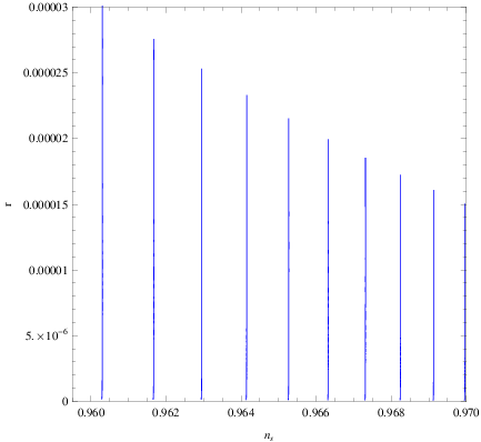
Having the functional form of the observational indices as functions of the -foldings and of the parameters given in Eqs. (24) and (25), we can directly confront the Einstein Gauss-Bonnet theory (17)-(18) with the observational data (15) and (16). A thorough analysis indicates that the parameter space is quite large and it allows the theory to be compatible with the observational data for a wide range of the parameter values. For example by choosing , and , , we obtain and , which are both compatible with the observational data. Also the canonical scalar field theory can also be compatible with the observational data, for example if , and for and , we get and which are also compatible with the observational constraints (15) and (16). Therefore, the Einstein Gauss-Bonnet theory of quintessential inflation enlarges the range of parameter values which render the model compatible with the observational data. This can also be seen in Fig. 1, where we have presented the parametric plot of the spectral index and of the tensor-to-scalar ratio as a function of the parameter , for , and for with step 0.0009 and .
Consider now the case that and are assumed to be,
| (26) |
In this case, the slow-roll indices read,
| (27) |
and the observational indices are equal to,
| (28) | ||||
From the functional form of the slow-roll indices as functions of the scalar field , namely Eq. (27), it is obvious that the slow-roll era is realized for small values of the scalar field. Following the procedure of the previous case, the observational indices as functions of the -foldings number are,
| (29) | ||||
| (30) |
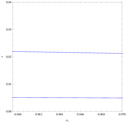
As in the previous case, the model (26) can also be compatible with the observational constraints on inflation, for a wide range of parameter values. In fact, the viability of the canonical scalar quintessential inflation model is enlarged. In Fig. 2 we present the parametric plot of the spectral index and of the tensor-to-scalar ratio as a function of the parameters and , with and . The different lines correspond to various values of the parameters and in the ranges with step 0.0001 and .
Now having discussed the inflationary properties of the Einstein Gauss-Bonnet extended quintessential inflationary models, what remains is to examine the late-time properties. The canonical scalar field quintessential model describes an accelerating late-time evolution, so it is vital to investigate the late-time behavior of the Einstein Gauss-Bonnet extensions we discussed earlier. This is the subject of the next section.
III Late-time Evolution of Quintessential Einstein Gauss-Bonnet Models
In the previous section we demonstrated how the single canonical scalar field quintessential inflation scenario is modified in the context of a simple Einstein Gauss-Bonnet extension. What now remains is to investigate the late-time properties of the Einstein Gauss-Bonnet quintessential inflation scenario. To this end, we shall make use of the redshift parameter, which is defined in terms of the scale factor as , where we have set the value of the scale factor at present time equal to one, that is . For the late-time evolution study we shall focus on the behavior of the deceleration parameter which in terms of the Hubble rate is defined as follows,
| (31) |
and of the total effective equation of state parameter (EoS) which is defined below,
| (32) |
For the purposes of our study we shall investigate the behavior of the above physical quantities as functions of the redshift, for redshifts in the range , which means that we look back in our Universe’s past for at least billion years. For the CDM model, the deceleration to acceleration transition occurs for , given that and . The study we shall perform in this section is purely numerical, so we shall express the gravitational equations of motion as functions of the redshift , so by using the following transformation rules for the derivative,
| (33) |
and also by assuming the presence of a dark matter fluid with energy density , the gravitational equations of motion become,
| (34) | ||||
| (35) | ||||
where , and are defined as follows,
| (36) |
and the primes in Eq. (34)-(35) denote differentiation with respect to the redshift . The differential equations (34)-(35) can be solved numerically, so we shall perform a thorough analysis for both the models (17)-(18) and (26)-(27), by using various initial conditions. Recall that the inflationary era for both the aforementioned Einstein Gauss-Bonnet models occurs for small values of the scalar field, so at late-times the scalar field must take relatively large values. An examination of the behavior of the solutions corresponding to the differential equations (34)-(35), reveals that a deceleration to acceleration transition for small redshifts of the order can occur only if the “velocity” of the scalar field is negative and small.
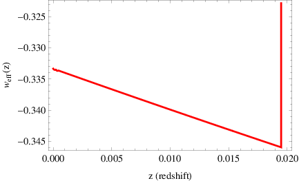
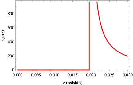
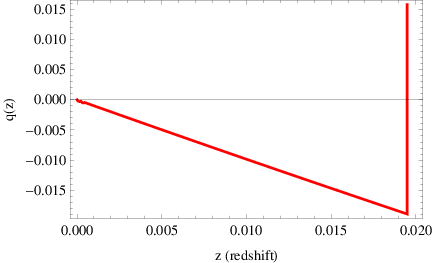
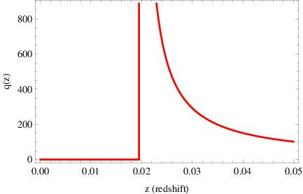
If on the other hand , the deceleration to acceleration transition occurs for which is unacceptable phenomenologically. For the model (17)-(18), the behavior of the deceleration parameter and of the total EoS parameter as functions of the redshift is presented in Figs. 3 and 4. For all the plots we have used the values , , and the initial conditions , and . Also an investigation of the behavior for various “velocities” of the scalar field at zero redshift, indicates that as the absolute value of the velocity drops, the redshift for which the deceleration to acceleration occurs increases. In the plots, the deceleration to acceleration transition occurs approximately at , and this depends strongly on the initial condition chosen for . From a phenomenological point of view, the behavior of the model at late times indicates that it can describe a decelerating era until some critical redshift is reached, at which point the Universe super-decelerates. After that critical redshift, the Universe accelerates in a decreasing rate until the present time era, in which the deceleration parameter approaches slowly the value zero. The same behavior occurs for the model (26)-(27), so we omit it. There seems to be a pattern of same behaviors for the Einstein Gauss-Bonnet models of the form , so we investigated another model of this form, with and . In this case the slow-roll inflationary era occurs for large values of the scalar field, so at late times the scalar field should in principle take small values. In Fig. 5 we present the deceleration (left) and the effective equation of state parameter (right), as functions of for the initial conditions , and and for and . As it can be seen in Fig. 5, the behavior of both and is quite similar to the previous quintessential Einstein Gauss-Bonnet models we studied.
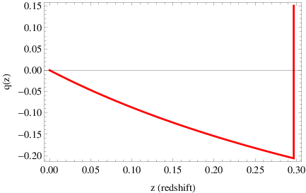
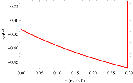
Thus we may conclude that the Einstein Gauss-Bonnet models with seem to produce the same phenomenology for late times, which indicates that the Universe decelerates until some redshift, and then after a steep deceleration point, an acceleration era occurs which has a decreasing rate. This result is different though from the CDM model, which describes a nearly constant acceleration rate until present time. Thus the resulting picture is not compatible with the CDM model, and although the early phenomenology of the models we studied is quite compatible with the observations, the late-time phenomenology is peculiar, however an accelerating evolution is generated.
IV Conclusions
In this paper we studied the early and late-time evolution of the Universe in the context of Einstein Gauss-Bonnet quintessential models. With regard to the early-time behavior, we presented the slow-roll formalism of the theory and we investigated if a viable inflationary era can be achieved. As we demonstrated, the spectral index and the tensor-to-scalar ratio corresponding to the models we studied can be compatible with the observational data coming from Planck and the BICEP2/Keck-Array data, for a wide range of the parameter values. Actually we showed that the viability of the quintessential models is enhanced in the context of the Einstein Gauss-Bonnet theory, in comparison to the single canonical scalar field case. With regard to the late-time era, all the models we studied result to a decelerating era until some critical redshift, at which point a super deceleration occurs, and eventually an acceleration era follows. Notably, the rate of the acceleration decreases until present time, and also the critical redshift at which the deceleration to acceleration transition occurs, crucially depends on the initial conditions chosen for the scalar field. The behavior of the models seems to be the same for all the models for which the scalar coupling to the Gauss-Bonnet scalar satisfies . Also, although a late-time acceleration era is produced for the quintessential Einstein Gauss-Bonnet model we studied, the evolution is different in comparison to the CDM model. In principle, the inclusion of higher order derivatives of the scalar field can alter this behavior, so in a future work we aim to examine this issue in more detail.
We need to note that what we tried to demonstrate here is the possibility to describe the inflationary and the dark energy eras, namely the two accelerating eras of our Universe, using the theoretical framework of Einstein-Gauss-Bonnet gravity. Such an idea is not new and it was firstly introduced in Ref. Nojiri:2003ft, in the context of gravity. However the difference is that in the Einstein-Gauss-Bonnet gravity, the behavior of the quintessential potential is peculiar and produces a super-decelerating era, absent in the context of gravity. To our opinion the gravity framework provides a much more solid phenomenological framework.
Finally, another question is whether the scalar field with such a quintessential potential used in this paper, can act as some dark matter component. This is a hard question to answer in brief, since up-to-date there is no evidence of particle dark matter, so perhaps in the context of some Chameleon theory of dark matter, this might be possible. Nevertheless the observational data seem to favor the particle nature for some or all of the components of dark matter, so we leave this question for a future work.
Acknowledgments
Financial support by the Research Committee of the Technological Education Institute of Central Macedonia, Serres, under grant SAT/ME/130319-111/17, is gratefully acknowledged.
References
- (1) A. H. Guth, Phys. Rev. D 23 (1981) 347. doi:10.1103/PhysRevD.23.347
- (2) A. D. Linde, Phys. Rev. D 49 (1994) 748 doi:10.1103/PhysRevD.49.748 [astro-ph/9307002].
- (3) A. D. Linde, Phys. Lett. 129B (1983) 177. doi:10.1016/0370-2693(83)90837-7
- (4) P. A. R. Ade et al. [Planck Collaboration], Astron. Astrophys. 594 (2016) A20 doi:10.1051/0004-6361/201525898 [arXiv:1502.02114 [astro-ph.CO]].
- (5) A. D. Linde, Lect. Notes Phys. 738 (2008) 1 [arXiv:0705.0164 [hep-th]].
- (6) D. S. Gorbunov and V. A. Rubakov, “Introduction to the theory of the early universe: Cosmological perturbations and inflationary theory,” Hackensack, USA: World Scientific (2011) 489 p;
- (7) A. Linde, arXiv:1402.0526 [hep-th];
- (8) D. H. Lyth and A. Riotto, Phys. Rept. 314 (1999) 1 [hep-ph/9807278].
- (9) S. Nojiri, S. D. Odintsov and V. K. Oikonomou, Phys. Rept. 692 (2017) 1 doi:10.1016/j.physrep.2017.06.001 [arXiv:1705.11098 [gr-qc]].
- (10) S. Nojiri, S.D. Odintsov, Phys. Rept. 505, 59 (2011);
- (11) S. Nojiri, S.D. Odintsov, eConf C0602061, 06 (2006) [Int. J. Geom. Meth. Mod. Phys. 4, 115 (2007)].
- (12)
S. Capozziello, M. De Laurentis,
Phys. Rept. 509, 167 (2011);
V. Faraoni and S. Capozziello, Fundam. Theor. Phys. 170 (2010). doi:10.1007/978-94-007-0165-6 - (13) A. de la Cruz-Dombriz and D. Saez-Gomez, Entropy 14 (2012) 1717 doi:10.3390/e14091717 [arXiv:1207.2663 [gr-qc]].
- (14) G. J. Olmo, Int. J. Mod. Phys. D 20 (2011) 413 doi:10.1142/S0218271811018925 [arXiv:1101.3864 [gr-qc]].
- (15) K. Dimopoulos, L. Donaldson Wood and C. Owen, Phys. Rev. D 97 (2018) no.6, 063525 doi:10.1103/PhysRevD.97.063525 [arXiv:1712.01760 [astro-ph.CO]].
- (16) C. van de Bruck, K. Dimopoulos, C. Longden and C. Owen, arXiv:1707.06839 [astro-ph.CO].
- (17) L. Areste Salo and J. de Haro, Eur. Phys. J. C 77 (2017) no.11, 798 doi:10.1140/epjc/s10052-017-5337-0 [arXiv:1707.02810 [gr-qc]].
- (18) A. Agarwal, R. Myrzakulov, M. Sami and N. K. Singh, Phys. Lett. B 770 (2017) 200 doi:10.1016/j.physletb.2017.04.066 [arXiv:1708.00156 [gr-qc]].
- (19) S. Ahmad, R. Myrzakulov and M. Sami, Phys. Rev. D 96 (2017) no.6, 063515 doi:10.1103/PhysRevD.96.063515 [arXiv:1705.02133 [gr-qc]].
- (20) C. Q. Geng, C. C. Lee, M. Sami, E. N. Saridakis and A. A. Starobinsky, JCAP 1706 (2017) no.06, 011 doi:10.1088/1475-7516/2017/06/011 [arXiv:1705.01329 [gr-qc]].
- (21) K. Dimopoulos and C. Owen, JCAP 1706 (2017) no.06, 027 doi:10.1088/1475-7516/2017/06/027 [arXiv:1703.00305 [gr-qc]].
- (22) J. de Haro, Gen. Rel. Grav. 49 (2017) no.1, 6 doi:10.1007/s10714-016-2173-8 [arXiv:1602.07138 [gr-qc]].
- (23) J. Haro and S. Pan, Int. J. Mod. Phys. D 27 (2018) no.05, 1850052 doi:10.1142/S0218271818500529 [arXiv:1512.03033 [gr-qc]].
- (24) M. Wali Hossain, R. Myrzakulov, M. Sami and E. N. Saridakis, Int. J. Mod. Phys. D 24 (2015) no.05, 1530014 doi:10.1142/S0218271815300141 [arXiv:1410.6100 [gr-qc]].
- (25) M. W. Hossain, R. Myrzakulov, M. Sami and E. N. Saridakis, Phys. Rev. D 89 (2014) no.12, 123513 doi:10.1103/PhysRevD.89.123513 [arXiv:1404.1445 [gr-qc]].
- (26) I. P. Neupane, Class. Quant. Grav. 25 (2008) 125013 doi:10.1088/0264-9381/25/12/125013 [arXiv:0706.2654 [hep-th]].
- (27) M. Sami and V. Sahni, Phys. Rev. D 70 (2004) 083513 doi:10.1103/PhysRevD.70.083513 [hep-th/0402086].
- (28) H. Tashiro, T. Chiba and M. Sasaki, Class. Quant. Grav. 21 (2004) 1761 doi:10.1088/0264-9381/21/7/004 [gr-qc/0307068].
- (29) K. Dimopoulos, Phys. Rev. D 68 (2003) 123506 doi:10.1103/PhysRevD.68.123506 [astro-ph/0212264].
- (30) K. Dimopoulos and J. W. F. Valle, Astropart. Phys. 18 (2002) 287 doi:10.1016/S0927-6505(02)00115-9 [astro-ph/0111417].
- (31) P. J. E. Peebles and A. Vilenkin, Phys. Rev. D 59 (1999) 063505 doi:10.1103/PhysRevD.59.063505 [astro-ph/9810509].
- (32) G. Cognola, E. Elizalde, S. Nojiri, S. Odintsov and S. Zerbini, Phys. Rev. D 75 (2007) 086002 doi:10.1103/PhysRevD.75.086002 [hep-th/0611198].
- (33) S. Nojiri, S. D. Odintsov and M. Sasaki, Phys. Rev. D 71 (2005) 123509 doi:10.1103/PhysRevD.71.123509 [hep-th/0504052].
- (34) S. Nojiri and S. D. Odintsov, Phys. Lett. B 631 (2005) 1 doi:10.1016/j.physletb.2005.10.010 [hep-th/0508049].
- (35) S. Nojiri, S. D. Odintsov and P. V. Tretyakov, Phys. Lett. B 651 (2007) 224 doi:10.1016/j.physletb.2007.06.029 [arXiv:0704.2520 [hep-th]].
- (36) M. Satoh and J. Soda, JCAP 0809 (2008) 019 doi:10.1088/1475-7516/2008/09/019 [arXiv:0806.4594 [astro-ph]].
- (37) M. Satoh, S. Kanno and J. Soda, Phys. Rev. D 77 (2008) 023526 doi:10.1103/PhysRevD.77.023526 [arXiv:0706.3585 [astro-ph]].
- (38) G. Hikmawan, J. Soda, A. Suroso and F. P. Zen, Phys. Rev. D 93 (2016) no.6, 068301 doi:10.1103/PhysRevD.93.068301 [arXiv:1512.00222 [hep-th]].
- (39) K. Bamba, A. N. Makarenko, A. N. Myagky and S. D. Odintsov, JCAP 1504 (2015) 001 doi:10.1088/1475-7516/2015/04/001 [arXiv:1411.3852 [hep-th]].
- (40) Z. Yi, Y. Gong and M. Sabir, arXiv:1804.09116 [gr-qc].
- (41) Z. K. Guo and D. J. Schwarz, Phys. Rev. D 80 (2009) 063523 doi:10.1103/PhysRevD.80.063523 [arXiv:0907.0427 [hep-th]].
- (42) Z. K. Guo and D. J. Schwarz, Phys. Rev. D 81 (2010) 123520 doi:10.1103/PhysRevD.81.123520 [arXiv:1001.1897 [hep-th]].
- (43) P. X. Jiang, J. W. Hu and Z. K. Guo, Phys. Rev. D 88 (2013) 123508 doi:10.1103/PhysRevD.88.123508 [arXiv:1310.5579 [hep-th]].
- (44) S. Koh, B. H. Lee, W. Lee and G. Tumurtushaa, Phys. Rev. D 90 (2014) no.6, 063527 doi:10.1103/PhysRevD.90.063527 [arXiv:1404.6096 [gr-qc]].
- (45) S. Koh, B. H. Lee and G. Tumurtushaa, Phys. Rev. D 95 (2017) no.12, 123509 doi:10.1103/PhysRevD.95.123509 [arXiv:1610.04360 [gr-qc]].
- (46) P. Kanti, R. Gannouji and N. Dadhich, Phys. Rev. D 92 (2015) no.4, 041302 doi:10.1103/PhysRevD.92.041302 [arXiv:1503.01579 [hep-th]].
- (47) P. Kanti, J. Rizos and K. Tamvakis, Phys. Rev. D 59 (1999) 083512 doi:10.1103/PhysRevD.59.083512 [gr-qc/9806085].
- (48) K. Nozari and N. Rashidi, Phys. Rev. D 95 (2017) no.12, 123518 doi:10.1103/PhysRevD.95.123518 [arXiv:1705.02617 [astro-ph.CO]].
- (49) S. D. Odintsov and V. K. Oikonomou, arXiv:1808.05045 [gr-qc].
- (50) S. Chakraborty, T. Paul and S. SenGupta, arXiv:1804.03004 [gr-qc].
- (51) P. A. R. Ade et al. [BICEP2 and Keck Array Collaborations], Phys. Rev. Lett. 116 (2016) 031302 doi:10.1103/PhysRevLett.116.031302 [arXiv:1510.09217 [astro-ph.CO]].
- (52) H. Noh and J. c. Hwang, Phys. Lett. B 515 (2001) 231 doi:10.1016/S0370-2693(01)00875-9 [astro-ph/0107069].
- (53) J. c. Hwang and H. Noh, Phys. Rev. D 71 (2005) 063536 doi:10.1103/PhysRevD.71.063536 [gr-qc/0412126].
- (54) J. c. Hwang and H. Noh, Phys. Rev. D 66 (2002) 084009 doi:10.1103/PhysRevD.66.084009 [hep-th/0206100].
- (55) S. Nojiri and S. D. Odintsov, Phys. Rev. D 68 (2003) 123512 doi:10.1103/PhysRevD.68.123512 [hep-th/0307288].