An Integrable Model for the Dynamics of Planetary Mean Motion ResonancesMatplotlib (Hunter 2007), NumPy (Oliphant 2006), REBOUND (Rein & Liu 2012), WHFast (Rein & Tamayo 2015), SciPy (Jones et al. 2001), Theano (Theano Development Team 2016)
Abstract
I consider the dynamics of mean motion resonances between pairs of co-planar planets and derive a new integrable Hamiltonian model for planets’ resonant motion. The new model generalizes integrable Hamiltonians previously derived for first-order resonances to the case of higher-order resonances by exploiting a surprising near-symmetry of the full, non-integrable Hamiltonians of higher-order resonances. Whereas past works have frequently relied on truncated disturbing function expansions to derive integrable approximations to resonant motion, I show that no such expansion is necessary to derive an integrable model. This enables the new model to accurately capture the dynamics of both first- and higher-order resonances for eccentricities up to orbit-crossing. I demonstrate that predictions of the new integrable model agree well with numerical integrations of resonant planet pairs. Finally, I explore the secular evolution of resonant planets’ eccentricities. I show that the secular dynamics are governed by conservation of an AMD-like quantity. I also demonstrate that secular frequencies depend on planets’ resonant libration amplitude and this generally gives rise to a secular resonance inside the mean motion resonance at large libration amplitudes. The integrable model derived in this work can serve as a framework for analyzing the dynamics of planetary MMRs in a wide variety of contexts.
Keywords:
celestial mechanics — keyword2 — keyword3I Introduction
Mean-motion resonances (MMRs) occur in a wide variety of contexts in celestial mechanics. Prominent examples in our own solar system include the 3:2 resonance between Neptune and Pluto, numerous resonances between giant planet satellites, and a wide variety of resonant phenomena in the asteroid and Kuiper belts (Yoder 1973; Peale 1976; Peale 1986; Peale 1999; Greenberg 1977; Malhotra 1988; Malhotra 1994, e.g.,). A number of giant planets discovered by radial velocity (RV) surveys are found in or near MMRs (Marcy et al. 2001; Goździewski & Maciejewski 2001; Lee & Peale 2002; Johnson et al. 2011; Wittenmyer et al. 2014; Trifonov et al. 2014; Trifonov et al. 2019, e.g.,). While MMRs are rare among multi-transiting super-Earths (Fabrycky et al. 2014), a handful of systems contain one or more resonant planet pair (Goździewski et al. 2016; Mills et al. 2016; Migaszewski et al. 2017; Panichi et al. 2019, e.g.,) including TRAPPIST-1’s 7-planet resonant chain (Gillon et al. 2017; Luger et al. 2017). An analytic understanding of resonant dynamics is desirable given the prevalence of MMRs in solar system and exoplanetary contexts.
Analytic treatments of resonant motion often rely on simplifying assumptions such as treating one of the planets as a massless test-particle, or assuming one of the orbits as (nearly) circular (Message 1966; Henrard & Lamaitre 1983; Lemaitre 1984; Peale 1986; Malhotra 1988; Murray & Dermott 1999, e.g.). These assumptions allow the resonant dynamics to be treated analytically because they yield equations of motion that depend on only one critical resonant angle. If, however, both planets have similar eccentricities then it is necessary to consider multiple critical resonant angles associated with various “sub-resonances” that are potentially all of equal importance. This obstacle is circumvented when treating the dynamics of first-order MMRs to lowest order in eccentricities due to the existence of an additional constant of motion (Sessin & Ferraz-Mello 1984) which can be constructed by means of a canonical transformation (Wisdom 1986; Henrard et al. 1986; Ferraz-Mello 2007; Batygin & Morbidelli 2013).
Beyond analytic treatments of MMRs in the circular restricted problem, a number of studies of MMRs have focused on computing families of periodic orbits (sometimes referred to as apsidal corotation resonances or ACRs) in the unrestricted planetary three-body problem that form the phase-space ‘skeleton’ around which more general (quasi-)periodic resonant orbits are built (Ferraz-Mello et al. 1993; Ferraz-Mello et al. 2003; Malhotra 2002; Beaugé et al. 2003; Lee 2004; Hadjidemetriou 2006; Michtchenko et al. 2006; Antoniadou & Voyatzis 2014, e.g.,). Other studies have provided detailed explorations of the global dynamics of specific MMRs in the unrestricted problem, often focusing on a particular planetary or satellite system (Michtchenko & Ferraz-Mello 2001; Callegari et al. 2004; Callegari et al. 2006; Callegari & Yokoyama 2007; Michtchenko et al. 2008a; Michtchenko et al. 2008b, e.g.,). Delisle et al. 2014 treat the dynamics of generic MMRs, both first- and higher order, and derive an integrable model for the motion in the vicinity of ACRs using the same canonical transformation that Wisdom 1986 and Henrard et al. 1986 employ for first-order resonances. The goal of this paper is to present a more general study of the global dynamics of generic MMRs.
This paper presents an integrable model that approximates the dynamics of generic MMRs in the planar unrestricted planetary three-body problem. This model was used previously in Hadden & Lithwick 2018 to derive a resonance-overlap criterion that predicts the onset of chaos for two massive, eccentric planets. An integrable treatment of higher-order resonances provides a key step in extending past criteria for the onset of chaos for nearly circular orbits (Wisdom 1980; Deck et al. 2013), based on the overlap of first-order resonances, to the case of eccentric planets for which higher-order resonances play an important role. Here I derive the integrable model for arbitrary-order MMRs and explore some aspects of the secular evolution of resonant planets. The model is derived in essentially the same manner as Delisle et al. 2014’s, utilizing the canonical transformation transformation of Wisdom 1986 and Henrard et al. 1986 to concentrate the resonant dynamics in a single “mode”. However, I show that this model provides a surprisingly accurate global description of the resonant dynamics and need not be restricted to the vicinity of an ACR as Delisle et al. 2014 assume.
This paper is organized as follows: I derive the integrable model for resonant motion in Section II. Section III compares the the integrable model with numerical integrations of resonant planet pairs. Section IV explores the secular evolution of resonant planet pairs. Finally, I conclude with a summary in Section V.
II An Integrable Model for Mean Motion Resonances
In this section I derive an integrable model for the dynamics of two massive planets in or near an MMR of arbitrary order. I consider a pair of planets with masses orbiting in or near a : resonance with around a star of mass . In Section II.1, I present a Hamiltonian model governing the resonant dynamics of the planet pair. In Section II.2, I show that, working to leading order in eccentricity, the resonant dynamics are well-approximated as a one-degree-of-freedom system. In Section II.3, I show that the one-degree-of-freedom approximation holds even when accounting for terms beyond leading order in eccentricity.
II.1 Formulation of Resonance Hamiltonian
The Hamiltonian governing the dynamics of a resonant planet pair, in terms of the canonical modified Delaunay variables (Morbidelli 2002, e.g.,)
where , and their conjugate angle variables , (with referring to the inner and outer planet, respectively) is
| (1) |
where
| (2) |
and
| (3) |
where , the resonant disturbing function, is a function of , the planets’ eccentricities and longitudes of periapse, and . The resonant disturbing function is defined as
| (4) |
where the integration variable is , and are the planets’ position vectors, and the secular component of the disturbing function,
has been subtracted in order to isolate purely resonant interactions.11 1 The indirect component of the disturbing function, represented by an additional term , in the integrand of Equation (4) has been omitted as it does not contribute to the averaged disturbing function for the resonances interior to the 2:1 MMR considered in this paper. Orbital elements appearing in are considered as functions of the canonical Poincare variables in the definition of (Eq. 3).
Frequently one works with an expansion of in powers of eccentricity truncated at some maximum order (Laskar & Robutel 1995, e.g.). In Section II.2, I approximate by the leading-order terms of such an expansion which for a th order resonance are . Alternatively, Equation (4) can be integrated numerically by evaluating the planets’ position vectors, and , as functions of the mean longitudes, and , as well as the planets’ eccentricities, and longitudes of periapse, , in the integrand (Schubart 1966, e.g.,). This approach is taken in Section II.3.
The Hamiltonian in Equation (1) has four dynamical degrees of freedom. Therefore, three integrals of motion (in addition to the total energy) are required to derive an integrable model for the motion. I derive three such (approximately) conserved quantities below via a series of canonical transformations. Before proceeding through any canonical transformations, however, I expand the Hamiltonian, Equation (1), about an exactly resonant configuration and re-scale the momenta and energy in order to make the derivation less cumbersome. Defining a reference semi-major axis, , near the outer planet’s initial semi-major axis, I choose units so that . With this reference semi-major axis defined, the Hamiltonian and all canonical momenta are re-scaled so that
are the new Hamiltonian and canonical momenta. I also define as the semi-major axis corresponding to the nominal : interior resonance with a planet at . Next, I transform the canonical momenta conjugate to by adding a constant so that the new momenta are
| (5) |
I assume that the variations on the planets’ semi-major axes are small and expand to second order in so that the Keplerian component of the Hamiltonian, Equation (2), becomes
| (6) |
where and Equation (3) becomes where is of order the planets’ mass ratio relative to the star. Finally, I will make the common approximation of ignoring temporal variations of the semi-major axes in the resonant Hamiltonian terms and always evaluate at .
Noting that the planets’ mean longitudes only appear in in the combination , we can reduce the number of degrees of freedom through the canonical transformation generated by the type-2 generating function
where is a constant whose value is chosen to eliminate terms linear in from the transformed Hamiltonian. The canonical transformation yields the conserved quantity , since its conjugate angle does not appear in the Hamiltonian. After dropping constant terms the transformed Hamiltonian becomes
| (7) |
where
| (8) |
The distance of the planets from exact commensurability is related to the new canonical momentum, , by
| (9) | |||||
II.2 Reduction to one degree of freedom
Assuming the planets’ eccentricities are small, the resonant dynamics can be approximated by taking the leading-order terms of an expansion of in powers of eccentricity. To leading order,
| (10) | |||||
where the are combinations of Laplace coefficients and their derivatives (Murray & Dermott 1999; Morbidelli 2002, e.g.,), the complex conjugates of the planets’ complex eccentricities, and ‘’ denotes the complex conjugate of the preceding term. Thus, to leading order in eccentricity, , contains distinct “sub-resonances” with resonant angles
for so it seems that there is no simple canonical transformation that can reduce the Hamiltonian to dependence on a single resonant angle. This apparent difficulty can be surmounted by exploiting the surprising fact that, to an excellent approximation, the sum appearing in Equation (10) can be re-written as a single linear combination of and raised to the th power. In other words, there exist coefficients and such that
| (11) |
While no choice of and can make Equation (11) exact (except in the trivial case ), the approximation is an excellent one. Equation (11) presents an over-determined system of equations for the coefficients in terms of two unknowns, and . In this paper I determine values for and via least-squares regression by minimizing
| (12) |
which is the sum of the squared differences of monomial coefficients between the left- and right-hand side of Equation (11). Figure 1 plots a measure of the fractional error in the approximation Equation (11) for resonances between the 2:1 and 9:8 MMRs up to order , showing that the agreement is excellent and improves with both closer planet spacings and higher resonance order. The dynamical origins of the approximate equality expressed by Equation (11) are discussed in Section II.4.
In light of Equation (11), I define
| (13) |
so that Equation (10) approximately reduces to
| (14) |
and is independent of and . For all MMRs interior to the 2:1 MMR, so that is roughly the vector difference of the planet pair’s eccentricity vectors represented in the complex plane. The ratio is more precisely fit as the power-law , which is plotted in the bottom panel of Figure 1. This approximation does not apply to the 2:1 MMR itself due to the presence of indirect terms in the disturbing function (Murray & Dermott 1999, e.g.,).
Now that is expressed via Equation (14) in terms of a single cosine term, we are in a position to derive an integrable Hamiltonian model. First, we need to express and in terms of the canonical variables. This is accomplished by first noting that, to leading order in eccentricity, and . Then, the canonical rotation transformation
| (15) |
where
| and |
defines new conjugate momentum-coordinate pairs and (Wisdom 1986; Henrard et al. 1986; Batygin & Morbidelli 2013; Delisle et al. 2014). We now have and the resonant component of the Hamiltonian becomes
| (16) |
The Hamiltonian is independent of both and so the complex quantity
| (17) |
is approximately conserved by the resonant dynamics.22 2 The reader is cautioned that, while , it is not the case that . Instead, is given by a linear combination of and . In the limit that one planet’s mass vanishes, Equation (17) implies the conservation of the massive planet’s eccentricity.
It is now straightforward to reduce the system to a single degree of freedom using the canonical transformation generated by
| (18) |
yielding and as a new canonical momentum-coordinate pair along with and as conserved quantities with conjugate cyclic coordinates and , respectively.33 3 is strictly conserved by the full resonant Hamiltonian, Equation (1) because the D’Alembert property of the disturbing function ensures that its conjugate variable, , does not appear explicitly in the Hamiltonian. This is most readily seen by considering Equation (17) in the limit where one of the masses vanishes: is then equal to the longitude of perihelion of the massive planet which cannot appear as an isolated cosine argument in a disturbing function expansion (Murray & Dermott 1999, e.g.,). Therefore, unlike , the conservation of does not rely on the accuracy of the approximation expressed in Equation (11). The transformed Hamiltonian is
| (19) |
where . Finally, Equation (19) gives an integrable one degree-of-freedom Hamiltonian for the resonant dynamics. Hamiltonians of the form given in Equation (19) have been studied extensively in the literature as models for resonant motion (Henrard & Lemaitre 1983; Lemaitre 1984, e.g.,). The dynamics are approximately pendulum-like, with oscillating about an equilibrium value of .
After the series of canonical transformations it is instructive to express the canonical variables and in terms of familiar orbital elements. Working back through the transformations, we have
| (20) |
Additionally, using Equation (9) and , the dynamical variables are related to the planets’ instantaneous period ratio by
| (21) |
II.3 Beyond the Leading Order Approximation
Hamiltonian (19) was derived by considering only the lowest-order terms from the expansion of the , Equation (4), in powers of the planets’ eccentricities. The derivation took advantage of a surprising near-symmetry exhibited by these lowest-order terms, expressed in Equation (11), that leads to the (approximate) conservation of . In fact, this near-symmetry persists even when higher order resonant terms are included in the Hamiltonian.
The resonant disturbing function can be computed without using a truncated expansion in eccentricities by evaluating Equation (4) via numerical quadrature. In the following, I evaluate and its derivatives numerically using a Gauss-Legendre quadrature rule. I utilize the exoplanet package’s (Foreman-Mackey et al. 2019) Kepler solver, based on algorithms by Nijenhuis 1991 and Markley 1995, in order to compute planets’ position vectors as functions of the canonical variables. Code for evaluating by numerical quadrature is available online at github.com/shadden/IntegrableModelforResonances.
The full resonant disturbing function can be represented as the cosine series (see Appendix A)
| (22) |
where, to leading order in eccentricities, the amplitudes so that amplitudes decrease with increasing and the terms with are generally the most important for a given (see Appendix A). (The sum of the exponents of and is equal to for while it is at least for or .) The approximation for used in Section II.2 to derive an integrable Hamiltonian (Equation 19) included only the term from the sum in Equation (22) and furthermore approximates this term, , by its leading-order piece .
If, more generally, the resonant disturbing function is approximated as
| (23) |
then it still depends only on a single resonant angle, and will remain approximately conserved by the resonant dynamics. Figure 2 shows that Equation (23) is in fact a remarkably good approximation of the resonant disturbing function even in cases where Equation (14) is not. The figure shows the magnitudes of Fourier amplitudes, , for three different resonances and a range of eccentricities. As the planets approach orbit-crossing, high-order Fourier coefficients decay more slowly and terms in Equation (22) with become increasingly important. However, generally remains larger than the next-largest by roughly an order of magnitude or more at each . In all but one case, with up to at least .
The sum in Equation (23) can be computed by simply evaluating with if fractional corrections of order to the amplitudes are ignored. Accordingly, the Hamiltonian governing the resonant dynamics can be approximated by the integrable Hamiltonian
| (24) |
where
is computed by numerically integrating Equation (4). This Hamiltonian is compared with -body results below in Section III.
II.4 Hill’s problem and the origin of the reducing transformation
Equation (11) expresses an apparently coincidental relationship between disturbing function coefficients that yields an approximately-conserved quantity, , and makes the derivation of the integrable approximation of the resonant dynamics possible. This naturally leads to the question: what near-symmetry of the underlying dynamics is responsible for the existence of this approximately-conserved quantity? Hill’s equations (Hill 1878) offer some insight into the answer.
As Henon & Petit 1986 note, Hill’s equations are not merely a limiting case of the circular restricted three-body problem as they do not place any restrictions on the eccentricities of the orbits under consideration nor do they require that one body’s mass vanish. Instead, Hill’s approximation only requires two bodies’ (i.e., the planets) masses be small compared to the primary (i.e., the star). Under Hill’s approximation, the small bodies’ motion is separated into the center-of-mass motion, which follows a Keplerian orbit with complex eccentricity , and the relative motion of the bodies, which evolves according to Hill’s equations. In particular, the evolution of the planets’ orbits under Hill’s approximation can be expressed in terms of a fictitious relative orbit with orbital elements that include a relative complex eccentricity, .
Building on the work of Henon & Petit 1986, Duncan et al. 1989 and Namouni et al. 1996 derive area-preserving maps that approximate the dynamics of a pair of planets by “stitching together” successive close encounters approximated by Hill’s equations. These area-preserving maps successfully reproduce resonant phase-space structure seen in -body integrations (though, as Namouni et al. 1996 demonstrate, the mapping must include sufficiently high-order terms in eccentricity to successfully capture the phase-space structure of high-order resonances for eccentric planets). Therefore, to the degree that resonant dynamics are accurately approximated by these ‘encounter maps’ the resonant dynamics should, just like Hill’s equations, only depend on the relative eccentricity, .
In the limit , the coefficients so that and the conserved quantity (Equation 17). Therefore, in the close-spacing limit, the integrable model depends only on the complex relative eccentricity and conserves the complex eccentricity of the center-of-mass orbit like Hill’s equations.
III Comparison with Numerical Integrations
Here I compare the integrable resonance models derived in Sections II with -body integrations. All -body integrations throughout this paper are done with the WHFast integrator (Rein & Tamayo 2015) based on the symplectic mapping algorithm of Wisdom & Holman 1991 and implemented in the REBOUND code (Rein & Liu 2012). Integration step sizes are set to 1/30th of the perihelion passage timescale of the inner planet, defined as where is the rate of change of the true anomaly at pericenter (Wisdom 2015). While the analytic model applies to all MMRs of any order interior to the 2:1 MMR, the numerical examples throughout the rest of the paper will focus on the 3:2, 5:3, and 8:5 MMRs.44 4 Technically, the canonical variables appearing in the resonance Hamiltonian introduced in Equation (1) differ from standard canonical variables of the full -body problem by a near-identity transformation (see, e.g., Deck et al. 2013, for an explicit construction of this transformation to first order in planet masses and eccentricities). I do not make any corrections for this difference when comparing -body integration with the analytic model as they are negligible in the cases studied here. However, this effect becomes more significant as MMRs’ orbital separations become closer.
I show in Appendix A that all resonances of a given order exhibit essentially the same functional dependence when scaled by , the value at which the planets’ orbits first intersect, so these resonances serve as representative examples for all first-, second-, and third order resonances. The value of is determined for fixed values of , , and by solving for the value of for which the planets’ complex eccentricities satisfy
(Kholshevnikov & Vassiliev 1999). For closely spaced planets, approximating and writing gives to first order in and .
Figure 3 shows some examples of the resonant motion of pairs of massive planets in different resonances, comparing the simple model derived to leading order in eccentricity in Section II.2 with -body integrations. The analytic model shows good general agreement with the -body results; the most significant differences being slight deviations in the predicted libration frequencies, especially in the case of the first-order 3:2 MMR. In this case, the disagreement is primarily due to truncating at first order in ; the disagreement is greatly reduced by including the additional term from in integrations of the analytic model.
Figure 4 compares the numerically-computed Hamiltonian model, Equation (24), with -body integrations. The Hamiltonian model shows excellent agreement with the -body integrations. The -body integrations were initialized with while Hamiltonian (24) is computed assuming , confirming that the resonant dynamics are nearly independent of . A moderately large value of was chosen in Figure 4 in order to illustrate a regime where contours of the numerically-averaged Hamiltonian differ significantly from those of the simple Hamiltonian (19).
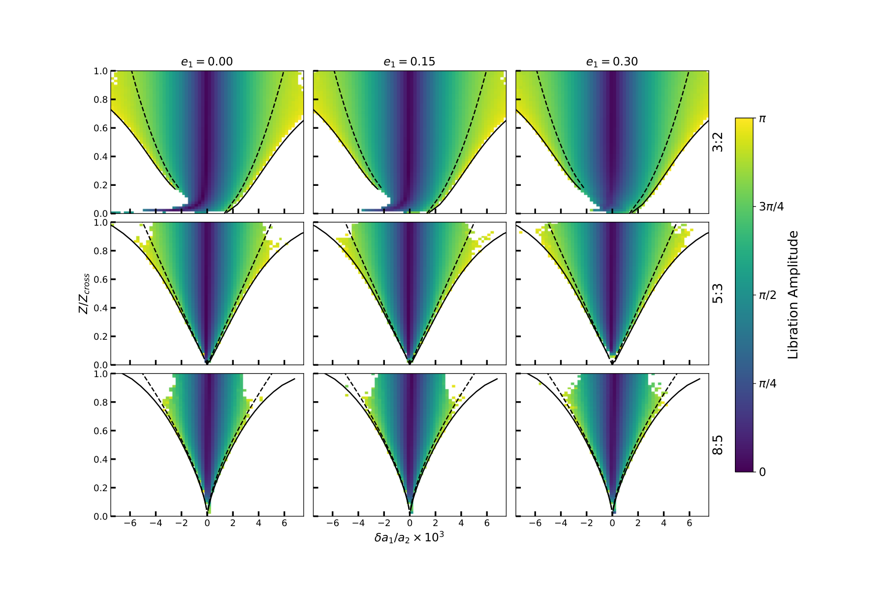
The analytic model predicts that systems with different individual eccentricities but the same combined eccentricity, , will have the same resonant dynamics. Figure 5 illustrates this by comparing a series of -body integrations at different resonances that are initialized with different individual planet eccentricities but equivalent s. Each panel shows a map of the resonant angle libration amplitude, measured from -body integrations. Different resonances are plotted in each row, and each column corresponds to a different initial eccentricity of the inner planet. The libration amplitude maps for a given resonance are nearly indistinguishable over the wide range of inner planet eccentricity spanning to .
Resonance widths predicted with the simple leading-order model, Equation (19), as well as the numerically-averaged model, Equation (24) are shown in each panel. Separatrices are computed as follows: for a fixed value of , the unstable fixed point of is located at by numerically solving for the value of that maximizes . The maximum, , determines the energy of the separatrix trajectory. The maximal width of the separatrix is then determined by solving for . The values of and are then converted to and using Equations (20) and (21). The most significant differences between the leading-order model and the full numerically-averaged model occurs for the 3:2 first-order MMR.
IV Secular Evolution
In this section I consider resonant dynamics with a more complete Hamiltonian model that includes secular terms. Secular dynamics inside MMRs have been examined by numerous previous studies, usually with applications to small solar system bodies (Kozai 1985; Wisdom 1985; Yoshikawa 1989; Morbidelli & Moons 1993; Moons & Morbidelli 1995; Gallardo et al. 2012; Saillenfest et al. 2016, e.g.,), though extra-solar contexts have also been considered (Beust & Morbidelli 1996; Batygin & Morbidelli 2013; Pichierri et al. 2017, e.g.,). The treatment presented here is similar to Batygin & Morbidelli 2013, though here I generalize to MMRs of arbitrary order.55 5 Batygin & Morbidelli 2013 also truncate the resonant disturbing function at first eccentricity whereas here I evaluate the resonant disturbing by numerical quadrature. This can yield some differences in the quantitative predictions of the model as already seen, for example, in Figure 5.
In Appendix B I show that, to leading order in eccentricity, secular interactions between a planet pair are governed by the Hamiltonian
| (25) |
where coefficients and depend on and the planets’ mass ratio, . Explicit expressions are given in Appendix B.
The inclusion of secular terms has introduced an explicit dependence on to the Hamiltonian so that is no longer a conserved quantity. However, is still conserved. The conserved quantity is analogous to the ‘angular momentum deficit’, given by , which is a conserved quantity under purely secular evolution in the absence of MMRs (Laskar 1997; Laskar 2000, e.g.,). Roughly speaking, resonant planets conserve their ‘libration-averaged’ AMD since and the resonant dynamics cause to oscillate about an equilibrium value .
If, initially, , then for all time and the Hamiltonian can be reduced to
| (26) |
so that the dynamics are completely integrable. In this case, the secular terms merely introduce a small shift to the center of the resonance through the ‘’ term. In general, when , the term
| (27) |
couples the two degrees of freedom and varies with time.
To further analyze the secular dynamics of resonant planets, I introduce the Arnold action-angle variables
| (28) |
of the integrable Hamiltonian , where is the resonant libration period, is time, and is a -periodic function of . I follow the semi-analytic procedure of Henrard 1990 to affect this transformation (Morbidelli & Moons 1993; Moons & Morbidelli 1995, see also).66 6 Numerical routines for performing the transformation are available online. After the transformation to action-angle variables, the Hamiltonian provides a mapping from the two action variables, and , to two dynamical frequencies and . Figure 6 compares values of , calculated with the semi-analytic procedure to frequencies measured from -body simulations using the FMFT algorithm of Šidlichovský & Nesvorný 1996. The agreement between the semi-analytic and -body results is quite good when is sufficiently far from zero. As I will show below, when the effect of introduces a secondary resonance that is responsible for the the abrupt changes in the secular frequencies seen in the -body results.
After transformation (28) the perturbing Hamiltonian becomes
| (29) |
where the
can be determined numerically (Henrard 1990, see). Thus, introduces secondary resonances in regions of phase space where for integer values of . The secular frequency is typically significantly smaller than the libration frequency so that only the resonance condition can be satisfied outside of a narrow region near the separatrix where . Accordingly, the secular dynamics are well-approximated by averaging over to obtain the Hamiltonian
| (30) |
describing an integrable, one degree-of-freedom system with as a conserved adiabatic invariant. (Batygin & Morbidelli 2013 also identify this adiabatic invariant in their treatment of first-order resonances, though they do not calculate it explicitly.) Plotting contours of constant for a collection of trajectories with fixed and , as in Figure 7, can be used to obtain a global picture of the secular dynamics. Note that far from the secular resonance will oscillate about its mean value with frequency and amplitude , as can be shown from the equations of motion after noting .
Figure 8 shows some representative maps illustrating the secular dynamics inside various resonances. Each panel shows a color map of the magnitude of the fractional variation in measured from -body simulations. Secular resonances are evident in each map. For the 3:2 and 5:3 MMRs with , the secular resonance appear near libration amplitudes of with increasing from 0 at the center of the resonance to large values towards the edges. In the 8:5 MMRs with , secular resonance occurs for all libration amplitudes at low .


Figure 9 shows the secular evolution for some representative initial conditions indicated in the middle column of Figure 8. Red trajectories show the secular evolution for systems with moderate initial resonant libration amplitudes outside of the secular resonance. The critical angle of the secular resonance, , circulates. These trajectories show small variations in the equilibrium value () about which resonant librations occur. Blue trajectories are selected deep in the secular resonance and show small oscillations about and again show minimal variations in their equilibrium value. Green trajectories are selected to lie at the edge of the secular resonance and the secular critical angle, , shows large-amplitude libration. These trajectories show large variations in their equilibrium over the libration period of the secular critical angle while the amplitude of their oscillations in remain roughly constant. As shown in top panels of Figure 9, these trajectories’ decrease in until, as a result of narrower resonance widths at lower values, the oscillations in nearly reach the resonance separatrix, at which point increases again.
These numerical examples serve to illustrate that the secular evolution of resonant planet pairs exhibit a rich dynamics. A more thorough analysis of the secular evolution of resonant planets exploring the possibility of chaotic motion is beyond the scope of the present work. However, before concluding I discuss some potential sources of secular chaos in MMRs identified by previous works. Batygin & Morbidelli 2013 discuss the possibility for chaos caused by the resonant trajectory intermittently encountering the separatrix over the course of secular evolution. Such secularly-induced chaos is apparently largely absent from the numerical examples presented in this paper: chaotic regions of phase space, shown in gray in Figure 8, are relatively small and concentrated near the separatrix (i.e., libration amplitudes ) at large eccentricities. Furthermore, it is unclear how much of this chaos is induced by secular modulations versus overlap with adjacent MMRs.77 7 In Batygin & Morbidelli 2013’s example exhibiting secularly-induced chaos, the planets are in the 2:1 MMR. Chaotic trajectories probably occupy a larger fraction of the phase space of this resonance compared to generic first-order MMRs because the 2:1 MMR disturbing function contains indirect terms that break the near-symmetry discussed in Section II.4. Morbidelli & Moons 1993 and Moons & Morbidelli 1995 present an extensive treatment of the secular dynamics of test-particles in MMRs with Jupiter and identify locations where resonant particles’ apsidal precession frequencies are commensurate with the external forcing frequencies and , the dominant harmonics in Jupiter’s secular eccentricity evolution. These secular resonances are analogous to the secular resonance identified here, though in the Jupiter-test particle case each MMR hosts two secular resonances corresponding to Jupiter’s two secular modes. Morbidelli & Moons 1993 and Moons & Morbidelli 1995 show that these two secular resonances overlap and lead to wide chaotic regions inside Jupiter’s MMRs. This chaos destabilizes resonant orbits and is partially responsible for the formation of the Kirkwood gaps. Multiple secular resonances inside MMRs would likewise exist for resonant planet pairs in systems hosting more than two planets due to the presence of additional secular frequencies in the system. The overlap of such resonances could lead to chaos and potentially destabilize resonant planet pairs in multi-planet systems.
V Summary
I derived analytic (Equation 19) and semi-analytic (Equation 24) integrable, one-degree-of-freedom Hamiltonian models for the dynamics of MMRs of arbitrary order between co-planar planets. Unlike many analytic models of MMRs, this model does not require that one of the planets be massless or on a circular orbit; the model only assumes co-planar planets on non-crossing orbits in or near a resonance interior to the 2:1 MMR. In Section III, I showed that this approximate model accurately describes the results of numerical integrations of resonant planet pairs. In Section IV, I examined the effects of longer-term secular evolution on the resonant dynamics. I showed that coupling between resonant planets’ libration amplitude and secular frequency leads to a secular resonance in certain regions of phase-space that can cause significant modulations of the planets’ eccentricities while elsewhere in phase space the secular evolution is characterized by small modulations of equilibrium eccentricities about which resonant oscillations occur.
The integrable model derived in this work provides a starting point for analyzing an array of dynamical phenomena such as resonant capture, resonances between mutually inclined planets, resonant chains, and secular evolution in systems of three or more planets containing resonant planet pairs.
References
- Antoniadou & Voyatzis (2014) Antoniadou, K. I., & Voyatzis, G. 2014, Ap&SS, 349, 657
- Batygin & Morbidelli (2013) Batygin, K., & Morbidelli, A. 2013, A&A, 556, A28
- Beaugé et al. (2003) Beaugé, C., Ferraz-Mello, S., & Michtchenko, T. A. 2003, ApJ, 593, 1124
- Beust & Morbidelli (1996) Beust, H., & Morbidelli, A. 1996, Icarus, 120, 358
- Callegari et al. (2004) Callegari, N., J., Michtchenko, T. A., & Ferraz-Mello, S. 2004, Celestial Mechanics and Dynamical Astronomy, 89, 201
- Callegari et al. (2006) Callegari, N., Ferraz-Mello, S., & Michtchenko, T. A. 2006, Celestial Mechanics and Dynamical Astronomy, 94, 381
- Callegari & Yokoyama (2007) Callegari, N., & Yokoyama, T. 2007, Celestial Mechanics and Dynamical Astronomy, 98, 5
- Cincotta et al. (2003) Cincotta, P. M., Giordano, C. M., & Simó, C. 2003, Physica D: Nonlinear Phenomena, 182, 151
- Deck et al. (2013) Deck, K. M., Payne, M., & Holman, M. J. 2013, ApJ, 774, 129
- Delisle et al. (2014) Delisle, J. B., Laskar, J., & Correia, A. C. M. 2014, A&A, 566, A137
- Duncan et al. (1989) Duncan, M., Quinn, T., & Tremaine, S. 1989, Icarus, 82, 402
- Fabrycky et al. (2014) Fabrycky, D. C., Lissauer, J. J., Ragozzine, D., et al. 2014, ApJ, 790, 146
- Ferraz-Mello (2007) Ferraz-Mello, S., ed. 2007, Astrophysics and Space Science Library, Vol. 345, Canonical Perturbation Theories - Degenerate Systems and Resonance
- Ferraz-Mello et al. (2003) Ferraz-Mello, S., Beaugé, C., & Michtchenko, T. A. 2003, Celestial Mechanics and Dynamical Astronomy, 87, 99
- Ferraz-Mello et al. (1993) Ferraz-Mello, S., Tsuchida, M., & Klafke, J. C. 1993, Celestial Mechanics and Dynamical Astronomy, 55, 25
- Foreman-Mackey et al. (2019) Foreman-Mackey, D., Barentsen, G., & Barclay, T. 2019, dfm/exoplanet: exoplanet v0.1.6, , , doi:10.5281/zenodo.2651251
- Gallardo et al. (2012) Gallardo, T., Hugo, G., & Pais, P. 2012, Icarus, 220, 392
- Gillon et al. (2017) Gillon, M., Triaud, A. H. M. J., Demory, B.-O., et al. 2017, Nature, 542, 456
- Goździewski & Maciejewski (2001) Goździewski, K., & Maciejewski, A. J. 2001, ApJ, 563, L81
- Goździewski et al. (2016) Goździewski, K., Migaszewski, C., Panichi, F., & Szuszkiewicz, E. 2016, MNRAS, 455, L104
- Greenberg (1977) Greenberg, R. 1977, Vistas in Astronomy, 21, 209
- Hadden & Lithwick (2018) Hadden, S., & Lithwick, Y. 2018, AJ, 156, 95
- Hadjidemetriou (2006) Hadjidemetriou, J. D. 2006, Celestial Mechanics and Dynamical Astronomy, 95, 225
- Henon & Petit (1986) Henon, M., & Petit, J. M. 1986, Celestial Mechanics, 38, 67
- Henrard (1990) Henrard, J. 1990, Celestial Mechanics and Dynamical Astronomy, 49, 43
- Henrard & Lamaitre (1983) Henrard, J., & Lamaitre, A. 1983, Celestial Mechanics, 30, 197
- Henrard & Lemaitre (1983) Henrard, J., & Lemaitre, A. 1983, Icarus, 55, 482
- Henrard et al. (1986) Henrard, J., Lemaitre, A., Milani, A., & Murray, C. D. 1986, Celestial Mechanics, 38, 335
- Hill (1878) Hill, G. W. 1878, American Journal of Mathematics, 1, 5
- Hunter (2007) Hunter, J. D. 2007, Computing in Science & Engineering, 9, 90
- Johnson et al. (2011) Johnson, J. A., Payne, M., Howard, A. W., et al. 2011, AJ, 141, 16
- Jones et al. (2001) Jones, E., Oliphant, T., Peterson, P., et al. 2001, SciPy: Open source scientific tools for Python, ,
- Kholshevnikov & Vassiliev (1999) Kholshevnikov, K. V., & Vassiliev, N. N. 1999, Celestial Mechanics and Dynamical Astronomy, 75, 67
- Kozai (1985) Kozai, Y. 1985, Celestial Mechanics, 36, 47
- Laskar (1997) Laskar, J. 1997, A&A, 317, L75
- Laskar (2000) —. 2000, Phys. Rev. Lett., 84, 3240
- Laskar & Robutel (1995) Laskar, J., & Robutel, P. 1995, Celestial Mechanics and Dynamical Astronomy, 62, 193
- Lee (2004) Lee, M. H. 2004, ApJ, 611, 517
- Lee & Peale (2002) Lee, M. H., & Peale, S. J. 2002, ApJ, 567, 596
- Lemaitre (1984) Lemaitre, A. 1984, Celestial Mechanics, 32, 109
- Luger et al. (2017) Luger, R., Sestovic, M., Kruse, E., et al. 2017, Nature Astronomy, 1, 0129
- Malhotra (1988) Malhotra, R. 1988, PhD thesis, Cornell Univ., Ithaca, NY.
- Malhotra (1994) —. 1994, Physica D Nonlinear Phenomena, 77, 289
- Malhotra (2002) —. 2002, ApJ, 575, L33
- Marcy et al. (2001) Marcy, G. W., Butler, R. P., Fischer, D., et al. 2001, ApJ, 556, 296
- Markley (1995) Markley, F. L. 1995, Celestial Mechanics and Dynamical Astronomy, 63, 101
- Message (1966) Message, P. J. 1966, in IAU Symposium, Vol. 25, The Theory of Orbits in the Solar System and in Stellar Systems, ed. G. I. Kontopoulos, 197
- Michtchenko et al. (2006) Michtchenko, T. A., Beaugé, C., & Ferraz-Mello, S. 2006, Celestial Mechanics and Dynamical Astronomy, 94, 411
- Michtchenko et al. (2008a) —. 2008a, MNRAS, 387, 747
- Michtchenko et al. (2008b) —. 2008b, MNRAS, 391, 215
- Michtchenko & Ferraz-Mello (2001) Michtchenko, T. A., & Ferraz-Mello, S. 2001, Icarus, 149, 357
- Migaszewski et al. (2017) Migaszewski, C., Goździewski, K., & Panichi, F. 2017, MNRAS, 465, 2366
- Mills et al. (2016) Mills, S. M., Fabrycky, D. C., Migaszewski, C., et al. 2016, Nature, 533, 509
- Moons & Morbidelli (1995) Moons, M., & Morbidelli, A. 1995, Icarus, 114, 33
- Morbidelli (2002) Morbidelli, A. 2002, Modern celestial mechanics : aspects of solar system dynamics (London: Taylor & Francis)
- Morbidelli & Moons (1993) Morbidelli, A., & Moons, M. 1993, Icarus, 102, 316
- Murray & Dermott (1999) Murray, C. D., & Dermott, S. F. 1999, Solar system dynamics (Cambridge, UK: Cambridge University Press)
- Namouni et al. (1996) Namouni, F., Luciani, J. F., Tabachnik, S., & Pellat, R. 1996, A&A, 313, 979
- Nijenhuis (1991) Nijenhuis, A. 1991, Celestial Mechanics and Dynamical Astronomy, 51, 319
- Oliphant (2006) Oliphant, T. E. 2006, A guide to NumPy, Vol. 1 (Trelgol Publishing USA)
- Panichi et al. (2019) Panichi, F., Migaszewski, C., & Goździewski, K. 2019, MNRAS, 485, 4601
- Peale (1976) Peale, S. J. 1976, Annual Review of Astronomy and Astrophysics, 14, 215
- Peale (1986) Peale, S. J. 1986, in Satellites, 159–223
- Peale (1999) —. 1999, ARA&A, 37, 533
- Pichierri et al. (2017) Pichierri, G., Morbidelli, A., & Lai, D. 2017, A&A, 605, A23
- Rein & Liu (2012) Rein, H., & Liu, S.-F. 2012, A&A, 537, A128
- Rein & Tamayo (2015) Rein, H., & Tamayo, D. 2015, MNRAS, 452, 376
- Saillenfest et al. (2016) Saillenfest, M., Fouchard, M., Tommei, G., & Valsecchi, G. B. 2016, Celestial Mechanics and Dynamical Astronomy, 126, 369
- Schubart (1966) Schubart, J. 1966, in IAU Symposium, Vol. 25, The Theory of Orbits in the Solar System and in Stellar Systems, ed. G. I. Kontopoulos, 187–193
- Sessin & Ferraz-Mello (1984) Sessin, W., & Ferraz-Mello, S. 1984, Celestial Mechanics, 32, 307
- Theano Development Team (2016) Theano Development Team. 2016, arXiv e-prints, abs/1605.02688
- Trifonov et al. (2014) Trifonov, T., Reffert, S., Tan, X., Lee, M. H., & Quirrenbach, A. 2014, A&A, 568, A64
- Trifonov et al. (2019) Trifonov, T., Stock, S., Henning, T., et al. 2019, AJ, 157, 93
- Šidlichovský & Nesvorný (1996) Šidlichovský, M., & Nesvorný, D. 1996, Celestial Mechanics and Dynamical Astronomy, 65, 137
- Wisdom (1980) Wisdom, J. 1980, AJ, 85, 1122
- Wisdom (1985) —. 1985, Icarus, 63, 272
- Wisdom (1986) —. 1986, Celestial Mechanics, 38, 175
- Wisdom (2015) —. 2015, AJ, 150, 127
- Wisdom & Holman (1991) Wisdom, J., & Holman, M. 1991, AJ, 102, 1528
- Wittenmyer et al. (2014) Wittenmyer, R. A., Tan, X., Lee, M. H., et al. 2014, ApJ, 780, 140
- Yoder (1973) Yoder, C. F. 1973, PhD thesis, UNIVERSITY OF CALIFORNIA, SANTA BARBARA.
- Yoshikawa (1989) Yoshikawa, M. 1989, A&A, 213, 436
Appendix A Fourier Representation of
In this Appendix I demonstrate some properties of the Fourier representation of the resonant disturbing function, , introduced in Equation (4). I begin by writing the full disturbing function as a Fourier series in the planets’ mean longitudes,
| (A1) |
where are complex amplitudes. Rewriting the combinations of the appearing in each Fourier term in terms of and introduced in Section II.1 gives
We see that only Fourier terms for which will give non-zero contributions when averaging the full disturbing function, Equation (A1), over to obtain . Retaining only these terms from the double sum in Equation (A1) and subtracting , the resonant disturbing function defined in Equation 4 is then
| (A2) |
The D’Alembert property (Murray & Dermott 1999; Morbidelli 2002, e.g.,) implies that the amplitudes are of the form
| (A3) |
where the ‘higher order terms’ are infinite series of monomials involving products of , , and with coefficients that depend on . Because the complex eccentricities and are each a linear combinations of and (Eq. 13), the monomials and can be written as linear combinations of the monomials and and . Similarly, can be written as a linear combination of the monomials with . Therefore
| (A4) |
where the new coefficients, , are linear combinations of the old and the ‘higher order terms’ are infinite series of monomials involving products of and and . Let us rewrite Equation (A4) as a generic Fourier series in and ,
| (A5) |
where the sum now extends from . Comparing terms in Equations (A4) and (A5), we have, to leading order, that . This is straightforward to see for . For and it is instructive to consider a concrete example: let’s take and corresponding to the Fourier term with complex phase in Equation (A5). The lowest-order term with complex phase appearing in Equation (A4) (and thus the leading order term in a Taylor expansion of ) occurs in the term of the sum as the product of , the latter term occurring in the series of monomials represented as ‘higher order terms’. Thus, the amplitude to leading order as claimed. Indeed, the leading-order term all for any and are formed by the product of , where , with and powers of occurring in the higher order terms of Equation (A4).
The results of Section II.3 can be restated as The functional dependence of these Fourier amplitudes, , on and is specific to the particular : MMR under consideration. However, the of distinct resonances of a given order are all well-approximated by a single function,
| (A6) |
where dependence on the particular resonance only enters only by determining the value of . A similar result was derived in Hadden & Lithwick 2018, where it was shown that the cosine-amplitudes of disturbing function terms in the restricted three-body problem can be approximated by where is the eccentricity of the test-particle and is the orbit crossing eccentricity. As this paper has demonstrated, the resonant dynamics of two eccentric planets is essentially identical to the dynamics of an eccentric test particle subject to a circular perturber after simply making the replacement so the cosine amplitudes appearing in Equation (23) should match those in the restricted problem after making this same replacement. Figure 10 compares numerically-computed coefficients with the approximation and illustrates that Hadden & Lithwick 2018’s approximation for disturbing function coefficients readily generalizes to resonances in the unrestricted problem. The coefficients have been scaled by to highlight deviations from the predicted leading-order behavior. Two sets of , one with and one with , are plotted for each resonance though the two values are indistinguishable in most instances, demonstrating that is nearly independent of .
Appendix B The Secular Hamiltonian
Here I derive the Hamiltonian governing secular interactions, Equation (25). The secular component of the disturbing function term, to leading order in eccentricities, is given by
| (B1) |
where and are combinations of Laplace coefficients, defined in in Appendix B of Murray & Dermott 1999.The secular Hamiltonian is given by after expressing in terms of canonical variables. Equation (15) relates the complex eccentricities, and , to the canonical variables introduced in Section II via the linear transformation
| (B2) |
Inserting (B2) into Equation (B1) and defining
gives the disturbing function in terms of canonical variables as
| (B3) |
so that
| (B4) |
where
| (B5) |
Finally, substituting , , and in Equation (B4) and dropping constant terms,
| (B6) |
which is the secular Hamiltonian introduced in Equation (25). \listofchanges