Double Robustness for Complier Parameters and a Semiparametric Test for Complier Characteristics

Rahul Singh Affiliation: Department of Economics, Massachusetts Institute of Technology, Affiliation: Cambridge, Massachusetts 02142, U.S.A. Affiliation: and Affiliation: Liyang Sun Affiliation: Center for Monetary and Financial Studies, Affiliation: Madrid, 28014, Spain

Abstract

We propose a semiparametric test to evaluate (i) whether different instruments induce subpopulations of compliers with the same observable characteristics on average, and (ii) whether compliers have observable characteristics that are the same as the full population on average. The test is a flexible robustness check for the external validity of instruments. We use it to reinterpret the difference in LATE estimates that Angrist and Evans 1998 obtain when using different instrumental variables. To justify the test, we characterize the doubly robust moment for Abadie 2003’s class of complier parameters, and we analyze a machine learning update to $\kappa$ weighting.

keywords: Instrumental Variable; Kappa Weight; Semiparametric Efficiency.

1 Introduction and related work

Average complier characteristics help to assess the external validity of any study that uses instrumental variable identification (Angrist and Evans 1998; Angrist and Fernández-Val 2013; Swanson and Hernán 2013; Baiocchi et al. 2014; Marbach and Hangartner 2020); whose treatment effects are we estimating when we use a particular instrument? We propose a semiparametric hypothesis test, free of functional form restrictions, to evaluate (i) whether two different instruments induce subpopulations of compliers with the same observable characteristics on average, and (ii) whether compliers have observable characteristics that are the same as the full population on average. It appears that no semiparametric test previously exists for this important question about the external validity of instruments, despite the popularity of reporting average complier characteristics in empirical research, e.g. Abdulkadiroğlu et al. 2014. By developing this hypothesis test, we equip empirical researchers with a new robustness check.

Equipped with this new test, we replicate, extend, and test previous findings about the impact of childbearing on female labor supply. In a seminal paper, Angrist and Evans 1998 use two different instrumental variables: twin births and same-sex siblings. The two instruments give rise to two substantially different local average treatment effect (LATE) estimates for the reduction in weeks worked due to a third child: -3.28 (0.63) and -6.36 (1.18), respectively, where the standard errors are in parentheses. Angrist and Fernández-Val 2013 attribute the difference in LATE estimates to a difference in average complier characteristics, i.e. a difference in average covariates for instrument specific complier subpopulations, writing that “twins compliers therefore are relatively more likely to have a young second-born and to be highly educated.” We find weak evidence in favor of the explanation that twins compliers are more likely to have a young second-born. We do not find evidence that twins compliers have a significantly different education level than same-sex compliers.

Our test is based on a new doubly robust estimator, which we call the automatic $\kappa$ weight (Auto- $\kappa$ ). To prove the validity of the test, we characterize the doubly robust moment function for average complier characteristics, which appears to have been previously unknown. More generally, we study low dimensional complier parameters that are identified using a binary instrumental variable $Z$ , which is valid conditional on a possibly high dimensional vector of covariates $X$ . Angrist et al. 1996 prove that identification of LATE based on the instrumental variable does not require any functional form restrictions. Using $\kappa$ weighting, Abadie 2003 extends identification for a broad class of complier parameters. As our main theoretical result, we characterize the doubly robust moment function for this class of complier parameters by augmenting $\kappa$ weighting with the classic Wald formula. Our main result answers the open question posed by Słoczyński and Wooldridge 2018 of how to characterize the doubly robust moment function for the full class, and it generalizes the well known result of Tan 2006, who characterizes the doubly robust moment function for LATE. By characterizing the doubly robust moment function for Abadie 2003’s class of complier parameters, we handle the new and economically important case of average complier characteristics.

The doubly robust moment function confers many favorable properties for estimation. As its name suggests, it provides double robustness to misspecification (Robins and Rotnitzky 1995) as well as the mixed bias property (Chernozhukov et al. 2018; Rotnitzky et al. 2021). As such, it allows for estimation of models in which the treatment effect for different individuals may vary flexibly according to their covariates (Frölich 2007; Ogburn et al. 2015). It also allows for nonlinear models (Abadie 2003; Cheng et al. 2009), which are often appropriate when outcome $Y$ and treatment $D$ are binary, and therefore avoids the issue of negative weights in misspecified linear models (Blandhol et al. 2022). Moreover, it allows for model selection of covariates and their transformations using machine learning, as emphasized in the targeted machine learning (van der Laan and Rubin 2006; Zheng and van der Laan 2011; Luedtke and van der Laan 2016; van der Laan and Rose 2018) and debiased machine learning (Belloni et al. 2017; Chernozhukov et al. 2016; Chernozhukov et al. 2018; Chernozhukov et al. 2021) literatures. A doubly robust estimator that combines both the $\kappa$ weight and Wald formulations not only guards against misspecification but also debiases machine learning. Finally, it is semiparametrically efficient in many cases (Hasminskii and Ibragimov 1979; Robinson 1988; Bickel et al. 1993; Newey 1994; Robins and Rotnitzky 1995; Hong and Nekipelov 2010).

The structure of the paper is as follows. Section 2 defines the class of complier parameters from Abadie 2003. Section 3 summarizes our main insight: the doubly robust moment for a complier parameter combines the familiar Wald and $\kappa$ weight formulations. Section 4 formalizes this insight for the full class of complier parameters. Section 5 develops the practical implication of our main insight: a semiparametric test to evaluate differences in observable complier characteristics, which we use to revisit Angrist and Evans 1998. Section 6 concludes. Appendix A proposes a machine learning estimator that we call the automatic $\kappa$ weight (Auto- $\kappa$ ), which we use to implement our proposed test.

This paper was previously circulated under a different title (Singh and Sun 2019).

2 Framework

Suppose we are interested in the effect of a binary treatment $D$ on a continuous outcome $Y$ in $\mathcal{Y}$ , a subset of $\mathbb{R}$ . There is a binary instrumental variable $Z$ available, as well as a potentially high dimensional covariate $X$ in $\mathcal{X}$ , a subset of $\mathbb{R}^{dim(X)}$ . We observe $n$ independent and identically distributed observations $(W_{i})$ , $(i=1,...,n)$ , where $W=(Y,D,Z,X^{\top})^{\top}$ concatenates the random variables. Following the notation of Angrist et al. 1996, we denote by $Y^{(z,d)}$ the potential outcome under the intervention $Z=z$ and $D=d$ . We denote by $D^{(z)}$ the potential treatment under the intervention $Z=z$ . Compliers are the subpopulation for whom $D^{(1)}>D^{(0)}$ . We place standard assumptions for identification.

Assumption 1 (Instrumental variable identification).

Assume

1.

Independence: $\{Y^{(z,d)}\},\{D^{(z)}\}\raisebox{0.50003pt}{\rotatebox[origin]{90.0}{$\models$}}Z\mid X$ for $d=0,1$ and $z=0,1$ .
2.

Exclusion: $\text{pr}\{Y^{(1,d)}=Y^{(0,d)}\mid X\}=1$ for $d=0,1$ .
3.

Overlap: $\pi_{0}(X)=\text{pr}(Z=1\mid X)$ is in $(0,1)$ .
4.

Monotonicity: $\text{pr}\{D^{(1)}\geq D^{(0)}\mid X\}=1$ and $\text{pr}\{D^{(1)}>D^{(0)}\mid X\}>0$ .

Independence states that the instrument $Z$ is as good as randomly assigned conditional on covariates $X$ . Exclusion imposes that the instrument $Z$ only affects the outcome $Y$ via the treatment $D$ . We can therefore simplify notation: $Y^{(d)}=Y^{(1,d)}=Y^{(0,d)}$ . Overlap ensures that there are no covariate values for which the instrument assignment is deterministic. Monotonicity rules out the possibility of defiers: individuals who will always pursue an opposite treatment status from their instrument assignment.

Angrist et al. 1996 prove identification of the local average treatment effect (LATE) using Assumption 1. Abadie 2003 extends identification for a broad class of complier parameters.

Definition 1 (General class of complier parameters (Abadie 2003)).

Let $g(y,d,x,\theta)$ be a measurable, real valued function such that $E\{g(Y,D,X,\theta)^{2}\}<\infty$ for all $\theta$ in $\Theta$ . Consider complier parameters $\theta_{0}$ implicitly defined by any of the following expressions:

1.

$E\{g(Y^{(0)},X,\theta)\mid D^{(1)}>D^{(0)}\}=0$ if and only if $\theta=\theta_{0}$ ;
2.

$E\{g(Y^{(1)},X,\theta)\mid D^{(1)}>D^{(0)}\}=0$ if and only if $\theta=\theta_{0}$ ;
3.

$E\{g(Y,D,X,\theta)\mid D^{(1)}>D^{(0)}\}=0$ if and only if $\theta=\theta_{0}$ .

We subsequently refer to these expressions as the three possible cases for complier parameters.

For a given instrumental variable $Z$ , one may define the average complier characteristics as a special case of Definition 1. This causal parameter summarizes the observable characteristics of the subpopulation of compliers who are induced to take up or refuse treatment $D$ based on the instrument assignment $Z$ . It is an important parameter to estimate because it aids the interpretation of LATE. As we will see in Section 5, this causal parameter can help to reconcile different LATE estimates obtained with different instruments.

Definition 2 (Average complier characteristics).

Average complier characteristics are $\theta_{0}=E\{f(X)\mid D^{(1)}>D^{(0)}\}$ for any measurable function $f$ of covariate $X$ that may have a finite dimensional, real vector value such that $E\{f_{j}(X)^{2}\}<\infty$ .

3 Key insight

3.1 Classic approaches: Wald formula and $\kappa$ weight

We provide intuition for our key insight that a doubly robust moment for a complier parameter has two components: the Wald formula and the $\kappa$ weight. For clarity, we focus on the familiar example of local average treatment effect (LATE) in this initial discussion: $\theta_{0}=E\{Y^{(1)}-Y^{(0)}\mid D^{(1)}>D^{(0)}\}$ . In subsequent sections, we study the entire class of complier parameters in Definition 1, including the new case of average complier characteristics.

Under Assumption 1, LATE can be identified as

\theta_{0}=\frac{E\left\{E(Y\mid Z=1,X)-E(Y\mid Z=0,X)\right\}}{E\left\{E(D\mid Z=1,X)-E(D\mid Z=0,X)\right\}}

following Frölich 2007. We call this expression the expanded Wald formula.

The direct Wald approach involves estimating the reduced form regression $E(Y\mid Z,X)$ and first stage regression $E(D\mid Z,X)$ , then plugging these estimates into the expanded Wald formula. Such an approach is called the plug-in, and it is valid only when both regressions are estimated with correctly specified and unregularized models. It is not a valid approach when either regression is incorrectly specified, leading to the name “forbidden regression” (Angrist and Pischke 2008). It is also invalid when the covariates are high dimensional and a regularized machine learning estimator is used to estimate either regression. The matching procedure of Frölich 2007 faces similar limitations.

In seminal work, Abadie 2003 proposes an alternative formulation in terms of the $\kappa$ weights

\kappa^{(0)}(W)=(1-D)\frac{(1-Z)-\{1-\pi_{0}(X)\}}{\{1-\pi_{0}(X)\}\pi_{0}(X)},\quad\kappa^{(1)}(W)=D\frac{Z-\pi_{0}(X)}{\{1-\pi_{0}(X)\}\pi_{0}(X)}

where $\pi_{0}(X)=\text{pr}(Z=1\mid X)$ is the instrument propensity score. The $\kappa$ weights have the property that

\theta_{0}=\omega^{-1}E\{\kappa^{(1)}(W)Y-\kappa^{(0)}(W)Y\},\quad\omega=E\left\{1-\frac{D(1-Z)}{1-\pi_{0}(X)}-\frac{(1-D)Z}{\pi_{0}(X)}\right\}.

In words, the mean of the product of $Y$ and $\kappa^{(d)}(W)$ gives, up to a scaling, the expected potential outcome $Y^{(d)}$ of compliers when treatment is $D=d$ . As an aside, Abadie 2003 also introduces a third weight $\kappa(W)$ for parameters that belong to the third case in Definition 1.

The $\kappa$ weight approach would involve estimating the propensity score $\hat{\pi}$ and plugging this estimate into the $\kappa$ weight formula. Intuitively, the $\kappa$ weight approach is like a multistage inverse propensity weighting. Impressively, it remains agnostic about the functional form of the reduced form regression $E(Y\mid Z,X)$ and first stage regression $E(D\mid Z,X)$ . It is valid only when $\hat{\pi}$ is estimated with a correctly specified and unregularized model. It is invalid if $\hat{\pi}$ is incorrectly specified or if covariates are high dimensional and a regularized machine learning estimator is used to estimate $\hat{\pi}$ . Moreover, the inversion of $\hat{\pi}$ can lead to numerical instability in high dimensional settings.

3.2 Doubly robust moment for a special case

Next, we introduce the moment function and doubly robust moment function formulations of LATE. For the special case of LATE, these formulations were first derived by Tan 2006 with the goal of addressing misspecification of the regressions and the propensity score. Consider the expanded Wald formula. Rearranging and using the notation $V=(Y,D)^{\top}$ as a column vector, $\gamma_{0}(Z,X)=E(V\mid Z,X)$ as a vector valued regression, and $\begin{pmatrix}1,&-\theta\end{pmatrix}$ as a row vector, we arrive at the moment function formulation of LATE:

E\left[\begin{pmatrix}1,&-\theta\end{pmatrix}\{\gamma_{0}(1,X)-\gamma_{0}(0,X)\}\right]=0\text{ if and only if }\theta=\theta_{0}.

Denote the the Horvitz-Thompson balancing weight as

\alpha_{0}(Z,X)=\frac{Z}{\pi_{0}(X)}-\frac{1-Z}{1-\pi_{0}(X)},\quad\pi_{0}(X)=\text{pr}(Z=1\mid X).

Tan 2006 shows that for LATE, the doubly robust moment function is

E\left[\begin{pmatrix}1,&-\theta\end{pmatrix}\{\gamma_{0}(1,X)-\gamma_{0}(0,X)\}+\alpha_{0}(Z,X)\begin{pmatrix}1,&-\theta\end{pmatrix}\{V-\gamma_{0}(Z,X)\}\right]=0\text{ if and only if }\theta=\theta_{0}.

The doubly robust formulation remains valid if either the vector valued regression $\gamma_{0}$ or propensity score $\pi_{0}$ is incorrectly specified.

3.3 A new synthesis that allows for machine learning

Our key observation is the connection between the $\kappa$ weight and the balancing weight $\alpha_{0}$ . This simple observation will allow us to characterize the doubly robust moment function for a broad class of complier parameters, generalizing Tan 2006 to the full class defined by Abadie 2003.

Proposition 1 ( $\kappa$ weight as balancing weight).

The $\kappa$ weights can be rewritten as

\displaystyle\kappa^{(0)}(W)=\alpha_{0}(Z,X)(D-1),\quad\kappa^{(1)}(W)=\alpha_{0}(Z,X)D,\quad\kappa(W)=1-\frac{D(1-Z)}{1-\pi_{0}(X)}-\frac{(1-D)Z}{\pi_{0}(X)}.

Proof.

Observe that

\alpha_{0}(z,x)=\frac{z}{\pi_{0}(x)}-\frac{1-z}{1-\pi_{0}(x)}=\frac{z-\pi_{0}(x)}{\pi_{0}(x)\{1-\pi_{0}(x)\}}

which proves the expression for $\kappa^{(0)}$ and $\kappa^{(1)}$ . Using these expressions, we have

\kappa(w)=\{1-\pi_{0}(x)\}\alpha_{0}(z,x)(d-1)+\pi_{0}(x)\alpha_{0}(z,x)d=1-\frac{d(1-z)}{1-\pi_{0}(x)}-\frac{(1-d)z}{\pi_{0}(x)}.

∎

Next, we formalize the sense in which the balancing weight $\alpha_{0}$ represents the functional $\gamma\mapsto E\left\{\begin{pmatrix}1,&-\theta\end{pmatrix}\gamma(1,X)-\gamma(0,X)\right\}$ that appears in the moment formulation of LATE and the extended Wald formula.

Proposition 2 (Balancing weight as Riesz representer).

$\alpha_{0}(z,x)$ is the Riesz representer to the continuous linear functional $\gamma\mapsto E\{\gamma(1,X)-\gamma(0,X)\}$ , i.e. for all $\gamma$ such that $E\{\gamma(Z,X)^{2}\}<\infty$ ,

E\{\gamma(1,X)-\gamma(0,X)\}=E\{\alpha_{0}(Z,X)\gamma(Z,X)\}.

Similarly, $Z/\pi_{0}(X)$ is the Riesz representer to the continuous linear functional $\gamma\mapsto E\{\gamma(1,X)\}$ , and $(1-Z)/\{1-\pi_{0}(X)\}$ is the Riesz representer to the continuous linear functional $\gamma\mapsto E\{\gamma(0,X)\}$ .

Proof.

This result is well known in semiparametrics. We provide the proof for completeness. Observe that

	$\displaystyle E\left\{\gamma(Z,X)\frac{Z}{\pi_{0}(X)}\mid X\right\}$	$\displaystyle=E\left\{\gamma(Z,X)\frac{1}{\pi_{0}(X)}\mid Z=1,X\right\}\text{pr}(Z=1\mid X)$
		$\displaystyle=E\left\{\gamma(Z,X)\frac{1}{\pi_{0}(X)}\mid Z=1,X\right\}\pi_{0}(X)=\gamma(1,X)$

and likewise

E\left\{\gamma(Z,X)\frac{1-Z}{1-\pi_{0}(X)}\mid X\right\}=\gamma(0,X).

Combining these two terms, we have by the law of iterated expectations

		$\displaystyle E\{\gamma(1,X)-\gamma(0,X)\}=\int\{\gamma(1,x)-\gamma(0,x)\}\mathrm{d}\text{pr}(x)$
		$\displaystyle=\int\left[E\left\{\gamma(Z,X)\frac{Z}{\pi_{0}(X)}\mid X=x\right\}-E\left\{\gamma(Z,X)\frac{1-Z}{1-\pi_{0}(X)}\mid X=x\right\}\right]\mathrm{d}\text{pr}(x)$
		$\displaystyle=E\left\{\gamma(Z,X)\frac{Z}{\pi_{0}(X)}\right\}-E\left\{\gamma(Z,X)\frac{1-Z}{1-\pi_{0}(X)}\right\}.$

∎

An immediate consequence of Proposition 2 is that

E\left\{\begin{pmatrix}1,&-\theta\end{pmatrix}\gamma(1,X)-\gamma(0,X)\right\}=E\left\{\alpha_{0}(Z,X)\begin{pmatrix}1,&-\theta\end{pmatrix}\gamma(Z,X)\right\}\text{ for any }\gamma.

In summary, Proposition 1 shows that the $\kappa$ weight is a reparametrization of the balancing weight $\alpha_{0}$ . Meanwhile, Proposition 2 shows that the balancing weight appears in the Riesz representer to the moment formulation of LATE, i.e. the expanded Wald formula. We conclude that the $\kappa$ weight is essentially the Riesz representer to the Wald formula. In seminal work, Newey 1994 demonstrates that a doubly robust moment is constructed from a moment formulation and its Riesz representer. Therefore the doubly robust moment for complier parameters must combine the Wald formula and the $\kappa$ weight.

With the general doubly robust moment function, one can propose flexible, semiparametric tests for complier parameters. In particular, the semiparametric tests may involve regularized machine learning for flexible estimation and model selection of (i) the regression $\hat{\gamma}$ in a way that approximates nonlinearity and heterogeneity, and (ii) the balancing weight $\hat{\alpha}$ in a way that guarantees balance. In Section 5, we instantiate such a test to compare observable characteristics of compliers.

As explained in Appendix A, we avoid the numerically unstable step of estimating and inverting $\hat{\pi}$ that appears in Tan 2006; Belloni et al. 2017; Chernozhukov et al. 2018. We replace it with the numerically stable step of estimating $\hat{\alpha}$ directly, extending techniques of Chernozhukov et al. 2018b to the instrumental variable setting. We call this extension automatic $\kappa$ weighting (Auto- $\kappa$ ), and demonstrate how it applies to the new and economically important case of average complier characteristics.

In summary, our main theoretical result allows us to combine the classic Wald and $\kappa$ weight formulations for the entire class of complier parameters in Definition 1, including average complier characteristics, while also updating them to incorporate machine learning.

4 The doubly robust moment

We now state our main theoretical result, which is the doubly robust moment for the class of complier parameters in Definition 1. This result formalizes the intuition of Section 3, and it justifies the hypothesis test in Section 5. It is convenient to divide the main result into two statements for clarity. Theorem 1 handles the first and second cases in Definition 1, while Theorem 2 handles the third case in Definition 1.

Theorem 1 (Cases 1 and 2).

Suppose Assumption 1 holds. Let $g(y,d,x,\theta)$ be a measurable, real valued function such that $E\{g(Y,D,X,\theta)^{2}\}<\infty$ for all $\theta$ in $\Theta$ .

1.

If $\theta_{0}$ is defined by $E[g\{Y^{(0)},X,\theta_{0}\}\mid D^{(1)}>D^{(0)}]=0$ , let $v(w,\theta)=(d-1)g(y,x,\theta).$
2.

If $\theta_{0}$ is defined by $E[g\{Y^{(1)},X,\theta_{0}\}\mid D^{(1)}>D^{(0)}]=0$ , let $v(w,\theta)=dg(y,x,\theta).$

Then the doubly robust moment function $\psi$ for $\theta_{0}$ is of the form

		$\displaystyle\psi(w,\gamma,\alpha,\theta)=m(w,\gamma,\theta)+\phi(w,\gamma,\alpha,\theta),\quad m(w,\gamma,\theta)=\gamma(1,x,\theta)-\gamma(0,x,\theta),$
		$\displaystyle\phi(w,\gamma,\alpha,\theta)=\alpha(z,x)\{v(w,\theta)-\gamma(z,x,\theta)\}$

where $\gamma_{0}(z,x,\theta)=E\{v(W,\theta)\mid z,x\}$ is a vector valued regression and $\alpha_{0}(z,x)=z/\pi_{0}(x)-(1-z)/\{1-\pi_{0}(x)\}$ is the Riesz representer of the functional $\gamma\mapsto E\{\gamma(1,X,\theta)-\gamma(0,X,\theta)\}$ .

Proof.

Consider the first case. Under Assumption 1, we can appeal to Abadie 2003:

0=E[g\{Y^{(0)},X,\theta_{0}\}\mid D^{(1)}>D^{(0)}]=\dfrac{E\{\kappa^{(0)}(W)g(Y,X,\theta_{0})\}}{\text{pr}\{D^{(1)}>D^{(0)}\}}.

Hence

	$\displaystyle 0$	$\displaystyle=E\{\kappa^{(0)}(W)g(Y,X,\theta_{0})\}=E\{\alpha_{0}(Z,X)(D-1)g(Y,X,\theta_{0})\}=E\{\alpha_{0}(Z,X)v(W,\theta_{0})\}$
		$\displaystyle=E\{\alpha_{0}(Z,X)\gamma_{0}(Z,X,\theta_{0})\}=E\{\gamma_{0}(1,X,\theta_{0})-\gamma_{0}(0,X,\theta_{0})\}$

appealing to the previous statement, Proposition 1, the definition of $v(W,\theta_{0})$ , the law of iterated expectations, and Proposition 2. Likewise for the second case. ∎

In the doubly robust moment function $\psi(w,\gamma,\alpha,\theta)=m(w,\gamma,\theta)+\phi(w,\gamma,\alpha,\theta)$ , we generalize our insight from Section 3. The first term $m(w,\gamma,\theta)$ is essentially a generalized Wald formula. The second term $\phi(w,\gamma,\alpha,\theta)$ is essentially a product between the $\kappa$ weight and a generalized regression residual. In the language of semiparametrics, we augment the $\kappa$ weight with the Wald formula. Equivalently, we debias the Wald formula with the $\kappa$ weight.

The doubly robust moment function $\psi$ remains valid if either $\gamma_{0}$ or $\alpha_{0}$ is misspecified, i.e.

0=E\{\psi(W,\gamma,\alpha_{0},\theta_{0})=E[\psi(W,\gamma_{0},\alpha,\theta_{0})\}\text{ for any }\gamma,\alpha.

In the former expression, $\gamma_{0}$ may be misspecified yet $\psi$ remains valid as an estimating equation. In the latter, $\alpha_{0}$ may be misspecified yet $\psi$ remains valid as an estimating equation. Theorem 1 demonstrates that all complier parameters in cases 1 and 2 of Definition 1 have a doubly robust moment function $\psi$ with a common structure. As such, we are able to analyze all of these causal parameters with the same argument. Case 3 of Definition 1 is more involved, but we show that it shares the common structure as well.

Theorem 2 (Case 3).

Suppose Assumption 1 holds. Let $g(y,d,x,\theta)$ be a measurable, real valued function such that $E\{g(Y,D,X,\theta)^{2}\}<\infty$ for all $\theta$ in $\Theta$ . If $\theta_{0}$ is defined by the moment condition $E\{g(Y,D,X,\theta_{0})\mid D^{(1)}>D^{(0)}\}=0$ , then the doubly robust moment function for $\theta_{0}$ is of the form

		$\displaystyle\psi(w,\tilde{\gamma},\tilde{\alpha},\theta)=m(w,\tilde{\gamma},\theta)+\phi(w,\tilde{\gamma},\tilde{\alpha},\theta),\quad m(w,\tilde{\gamma},\theta)=\gamma(z,x,\theta)-\gamma^{0}(1,x,\theta)-\gamma^{1}(0,x,\theta)$
		$\displaystyle\phi(w,\tilde{\gamma},\tilde{\alpha},\theta)=\{g(y,d,x,\theta)-\gamma(z,x,\theta)\}-\alpha^{0}(z,x)\{(1-d)g(y,d,x,\theta)-\gamma^{0}(z,x,\theta)\}$
		$\displaystyle\quad\quad\quad\quad\quad\quad-\alpha^{1}(z,x)\{dg(y,d,x,\theta)-\gamma^{1}(z,x,\theta)\}$

where $\tilde{\gamma}$ concatenates $(\gamma,\gamma^{0},\gamma^{1})$ and $\tilde{\alpha}$ concatenates $(\alpha^{0},\alpha^{1})$ . These functions are defined by

		$\displaystyle\gamma_{0}(z,x,\theta)=E\{g(Y,D,X,\theta)\mid z,x\},\quad\gamma_{0}^{0}(z,x,\theta)=E\{(1-D)g(Y,D,X,\theta)\mid z,x\},$
		$\displaystyle\gamma_{0}^{1}(z,x,\theta)=E\{Dg(Y,D,X,\theta)\mid z,x\},\quad\alpha_{0}^{0}(z,x)=z/\pi_{0}(x),\quad\alpha_{0}^{1}(z,x)=(1-z)/\{1-\pi_{0}(x)\}.$

Proof.

A similar argument extends to the third case. Under Assumption 1, we can appeal to Abadie 2003:

0=E\{g(Y,D,X,\theta_{0})\mid D^{(1)}>D^{(0)}\}=\dfrac{E\{\kappa(W)g(Y,D,X,\theta_{0})\}}{\text{pr}\{D^{(1)}>D^{(0)}\}}.

Hence

	$\displaystyle 0$	$\displaystyle=E\{\kappa(W)g(Y,D,X,\theta_{0})\}$
		$\displaystyle=E\left\{g(Y,D,X,\theta_{0})-\frac{Z}{\pi_{0}(X)}(1-D)g(Y,D,X,\theta_{0})-\frac{1-Z}{1-\pi_{0}(X)}Dg(Y,D,X,\theta_{0})\right\}$
		$\displaystyle=E\left\{\gamma_{0}(Z,X,\theta_{0})-\frac{Z}{\pi_{0}(X)}\gamma_{0}^{0}(Z,X,\theta_{0})-\frac{1-Z}{1-\pi_{0}(X)}\gamma_{0}^{1}(Z,X,\theta_{0})\right\}$
		$\displaystyle=E\{\gamma_{0}(Z,X,\theta_{0})-\gamma_{0}^{0}(1,X,\theta_{0})-\gamma_{0}^{1}(0,X,\theta_{0})\}$

appealing to the previous statement, Proposition 1, the definitions of $(\gamma_{0},\gamma_{0}^{0},\gamma_{0}^{1})$ together with the law of iterated expectations, and Proposition 2. ∎

This time, the doubly robust moment function $\psi$ remains valid if either $\tilde{\gamma}_{0}$ or $\tilde{\alpha}_{0}$ is misspecified, i.e.

0=E\{\psi(W,\tilde{\gamma},\tilde{\alpha}_{0},\theta_{0})=E[\psi(W,\tilde{\gamma}_{0},\tilde{\alpha},\theta_{0})\}\text{ for any }\tilde{\gamma},\tilde{\alpha}.

In the former expression, $\tilde{\gamma}_{0}$ may be misspecified yet $\psi$ remains valid as an estimating equation. In the latter, $\tilde{\alpha}_{0}$ may be misspecified yet $\psi$ remains valid as an estimating equation.

In Section 5, we translate this general characterization of the doubly robust moment into a practical hypothesis test to evaluate the external validity of instruments. In Appendix A, we translate this general characterization into general machine learning estimators for complier parameters, which we use to implement the hypothesis test. In particular, we consider direct estimation of the balancing weight, a procedure that we call automatic $\kappa$ weighting (Auto- $\kappa$ ).

5 A hypothesis test to compare observable characteristics

5.1 Corollaries for average complier characteristics

As a corollary, we characterize the doubly robust moment for average complier characteristics, which appears to have been previously unknown. Using the new doubly robust moment, we propose a hypothesis test, free of functional form restrictions, to evaluate (i) whether two different instruments induce subpopulations of compliers with the same observable characteristics on average, and (ii) whether compliers have observable characteristics that are the same as the full population on average.

Corollary 1 (Average complier characteristics).

The doubly robust moment for average complier characteristics is

\psi(w,\gamma,\alpha,\theta)=A(\theta)\{\gamma(1,x)-\gamma(0,x)\}+\alpha(z,x)A(\theta)\{v-\gamma(z,x)\},\quad A(\theta)=\begin{pmatrix}I,&-\theta\end{pmatrix}

where $v=\{df(x)^{\top},d\}^{\top}$ , $\gamma_{0}(z,x)=E(V\mid z,x)$ , and $\alpha_{0}(z,x)=z/\pi_{0}(x)-(1-z)/\{1-\pi_{0}(x)\}$ .

Proof.

The result is a special case of Corollary 3 in Appendix A. ∎

Suppose we wish to test the null hypothesis that two different instruments $Z_{1}$ and $Z_{2}$ induce complier subpopulations with the same observable characteristics on average. Denote by $\hat{\theta}_{1}$ and $\hat{\theta}_{2}$ the estimators for average complier characteristics using the different instruments $Z_{1}$ and $Z_{2}$ , respectively. One may construct machine learning estimators $\hat{\theta}_{1}$ and $\hat{\theta}_{2}$ based on the doubly robust moment function in Corollary 1. In Appendix A, we instantiate automatic $\kappa$ weight (Auto- $\kappa$ ) estimators of this type. The following procedure allows us to test the null hypothesis from some estimator $\hat{C}$ for the asymptotic variance $C$ of $\hat{\theta}=(\hat{\theta}^{\top}_{1},\hat{\theta}^{\top}_{2})^{\top}$ . In Appendix A, we provide an explicit variance estimator $\hat{C}$ based on Auto- $\kappa$ as well.

Algorithm 1 (Hypothesis test for difference of average complier characteristics).

Given $\hat{\theta}$ and $\hat{C}$ , which may be based on Auto- $\kappa$ as in Appendix A,

1.

Calculate the statistic $T=n(\hat{\theta}_{1}-\hat{\theta}_{2})^{\top}(R\hat{C}R^{\top})^{-1}(\hat{\theta}_{1}-\hat{\theta}_{2})$ where $R=\begin{pmatrix}I,&-I\end{pmatrix}$ .
2.

Compute the value $c_{a}$ as the $(1-a)$ quantile of $\chi^{2}\{dim(\theta_{1})\}$ .
3.

Reject the null hypothesis if $T>c_{a}$ .

Algorithm 1 can also test the null hypothesis that compliers have observable characteristics that are the same as the full population on average. $\hat{\theta}_{1}$ is as before, $\hat{\theta}_{2}=n^{-1}\sum_{i=1}^{n}f(X_{i})$ , and $\hat{C}$ updates accordingly.

Corollary 2 (Hypothesis test for difference of average complier characteristics).

If $\hat{\theta}=\theta_{0}+o_{p}(1)$ , $n^{1/2}(\hat{\theta}-\theta_{0})\rightsquigarrow\mathcal{N}(0,C)$ , and $\hat{C}=C+o_{p}(1)$ , then the hypothesis test in Algorithm 1 falsely rejects the null hypothesis $H_{0}$ with probability approaching the nominal level, i.e. $\text{pr}(T>c_{a}\mid H_{0})\rightarrow a.$

Proof.

The result is immediate from Newey and McFadden 1994. ∎

Corollary 2 is our main practical result: justification of a flexible hypothesis test to evaluate a difference in average complier characteristics. It appears that no semiparametric test previously exists for this important question about the external validity of instruments. By developing this hypothesis test, we equip empirical researchers with a new robustness check. This practical result follows as a consequence of our main insight in Section 3 and our main theoretical result in Section 4. In Appendix A, we verify the conditions of Corollary 2 for Auto- $\kappa$ under weak regularity assumptions.

5.2 Empirical application

With this practical result, we revisit a classic empirical paper in labor economics to test whether two different instruments induce different average complier characteristics. Angrist and Evans 1998 estimate the impact of childbearing $D$ on female labor supply $Y$ in a sample of 394,840 mothers, aged 21–35 with at least two children, from the 1980 Census. The first instrument $Z_{1}$ is twin births: $Z_{1}$ indicates whether the mother’s second and third children were twins. The second instrument $Z_{2}$ is same-sex siblings: $Z_{2}$ indicates whether the mother’s initial two children were siblings with the same sex. The authors reason that both $(Z_{1},Z_{2})$ are quasi random events that induce having a third child.

Table 1: Comparison of average complier characteristics

	Average age of second child				Average schooling of mother
	Twins	Same-sex	2 sided	1 sided	Twins	Same-sex	2 sided	1 sided
$\kappa$ weight	5.51	7.14	-	-	12.43	12.09	-	-
Auto- $\kappa$	4.52	6.92	0.13	0.07	9.84	12.10	0.54	0.27
Auto- $\kappa$ (S.E.)	(0.70)	(1.43)	-	-	(2.47)	(2.78)	-	-

Notes: S.E., standard error; Auto- $\kappa$ , automatic $\kappa$ weighting. See Supplement F for estimation details.

The two instruments give rise to two LATE estimates for the reduction in weeks worked due to a third child: -3.28 (0.63) for $Z_{1}$ and -6.36 (1.18) for $Z_{2}$ , where the standard errors are in parentheses. Angrist and Fernández-Val 2013 attribute the difference in LATE estimates to a difference in average complier characteristics, i.e. a difference in average covariates for instrument specific complier subpopulations. The authors use parametric $\kappa$ weights, report point estimates without standard errors, and conclude that “twins compliers therefore are relatively more likely to have a young second-born and to be highly educated.”

We replicate, extend, and test these previous findings. In their parametric $\kappa$ weight approach, Angrist and Fernández-Val 2013 estimate $\pi_{0}(X)$ using a logistic model with polynomials of continuous covariates. In our semiparametric Auto- $\kappa$ approach, we expand the dictionary to higher order polynomials, include interactions between the instrument and covariates, and directly estimate and regularize the balancing weights. Crucially, our main result allows us to conduct inference, and to test whether the instruments $Z_{1}$ and $Z_{2}$ induce differences in the observable complier characteristics suggested by previous work.

Table 1 summarizes results. In Columns 1, 2, 5, and 6, we find similar point estimates to Angrist and Fernández-Val 2013, given in Row 1. Columns 3, 4, 7, and 8 report $p$ values for tests of the null hypothesis that average complier characteristics are equal for the twins and same-sex instruments. We find weak evidence in favor of the explanation that twins compliers are more likely to have a young second-born. We do not find evidence that twins compliers have a significantly different education level than same-sex compliers.

6 Conclusion

We propose a semiparametric test to evaluate (i) whether two different instruments induce subpopulations of compliers with the same observable characteristics on average, and (ii) whether compliers have observable characteristics that are the same as the full population on average. This hypothesis test is a flexible and practical robustness check for the external validity of instrumental variables. We use the test to reinterpret the difference in LATE estimates that Angrist and Evans 1998 obtain when using two different instrumental variables. Specifically, we implement a machine learning update to $\kappa$ weighting that we call the automatic $\kappa$ weight (Auto- $\kappa$ ). To justify the test, we develop new econometric theory. Most notably, we characterize the doubly robust moment function for the entire class of complier parameters from Abadie 2003, answering an open question in the semiparametric literature in order to handle the new and economically important case of average complier characteristics.

Appendix A Automatic $\kappa$ weights

A.1 Estimation

In Section 4, we present our main theoretical result: the doubly robust moment function for the class of complier parameters in Definition 1. In this section, we propose a machine learning estimator based on this doubly robust moment function, which we call automatic $\kappa$ weighting (Auto- $\kappa$ ). We verify the conditions of Corollary 2 using Auto- $\kappa$ . In doing so, we provide a concrete end-to-end procedure to test whether two different instruments induce subpopulations of compliers with the same observable characteristics.

Debiased machine learning (Chernozhukov et al. 2016; Chernozhukov et al. 2018) is a meta estimation procedure that combines doubly robust moment functions (Robins and Rotnitzky 1995) with sample splitting (Klaassen 1987). Given the doubly robust moment function of some causal parameter of interest as well as machine learning estimators $(\hat{\gamma},\hat{\alpha})$ for its nonparametric components, debiased machine learning generates an estimator of the causal parameter.

Algorithm 2 (Debiased machine learning).

Partition the sample into subsets $(I_{\ell})$ , $(\ell=1,...,L)$ .

1.

For each $\ell$ , estimate $\hat{\gamma}_{-\ell}$ and $\hat{\alpha}_{-\ell}$ from observations not in $I_{\ell}$ .
2.

Estimate $\hat{\theta}$ as the solution to $n^{-1}\sum_{\ell=1}^{L}\sum_{i\in I_{\ell}}\psi(W_{i},\hat{\gamma}_{-\ell},\hat{\alpha}_{-\ell},\theta)|_{\theta=\hat{\theta}}=0.$

In Theorems 1 and 2, we characterize the doubly robust moment function $\psi$ for complier parameters. What remains is an account of how to estimate the vector valued regression $\hat{\gamma}$ and the balancing weight $\hat{\alpha}$ . Our theoretical results are agnostic about the choice of $(\hat{\gamma},\hat{\alpha})$ as long as they satisfy the rate conditions in Assumption 2 below. For example, $\hat{\gamma}$ could be a neural network.

For the balancing weight estimator $\hat{\alpha}$ , we adapt the regularized Riesz representer of Chernozhukov et al. 2018b, though one could similarly adapt the minimax balancing weight of Hirshberg and Wager 2021. This aspect of the procedure departs from the explicit inversion of the propensity score in Tan 2006; Belloni et al. 2017; Chernozhukov et al. 2018, and it improves numerical stability, which we demonstrate though comparative simulations in Supplement E. In particular, we project the balancing weight $\alpha_{0}(Z,X)$ onto the $p$ dimensional dictionary of basis functions $b(Z,X)$ . A high dimensional dictionary allows for flexible approximation, which we discipline with $\ell_{1}$ regularization.

Algorithm 3 (Regularized balancing weight).

Based on the observations in $I_{-\ell}$ ,

1.

Calculate $p\times p$ matrix $\hat{G}_{-\ell}=(n-n_{\ell})^{-1}\sum_{i\in I_{-\ell}}b(Z_{i},X_{i})b(Z_{i},X_{i})^{\top}$ ,
2.

Calculate $p\times 1$ vector $\hat{M}_{-\ell}=(n-n_{\ell})^{-1}\sum_{i\in I_{-\ell}}b(1,X_{i})-b(0,X_{i})$ ,
3.

Set $\hat{\alpha}_{-\ell}(Z,X)=b(Z,X)^{\top}\hat{\rho}_{-\ell}$ where $\hat{\rho}_{-\ell}=\argmin_{\rho}\rho^{\top}\hat{G}_{-\ell}\rho-2\rho^{\top}\hat{M}_{-\ell}+2\lambda_{n}|\rho|_{1}.$

We refer to our proposed estimator, which combines the doubly robust moment function from Theorems 1 and 2 with the meta procedure in Algorithm 2 and the regularized balancing weights in Algorithm 3, as automatic $\kappa$ weighting (Auto- $\kappa$ ) for complier parameters. The new doubly robust moment in Corollary 1 means that Auto- $\kappa$ applies to the new and economically important case of average complier characteristics.

A.2 Affine moments

When we verify the conditions of Corollary 2 using Auto- $\kappa$ , we focus on a sub-class of the complier parameters in Definition 1. This sub-class is rich enough to include several empirically important parameters, yet simple enough to avoid iterative estimation. The sub-class consists of complier parameters with affine moments, which we now define. The affine moment condition can be relaxed, but doing so incurs iterative estimation (Chernozhukov et al. 2016).

Definition 3 (Affine moment).

We say a doubly robust moment function $\psi$ is affine in $\theta$ if it takes the form

\psi(W,\gamma,\alpha,\theta)=A(\theta)\{\gamma(1,X)-\gamma(0,X)\}+\alpha(Z,X)A(\theta)\{V-\gamma(Z,X)\}

where $A(\theta)$ is a matrix with entries that are ones, zeros, or components of $\theta$ .

Next, we verify that several empirically important complier parameters have affine moments.

Definition 4 (Empirically important complier parameters).

Consider the following popular parameters.

1.

LATE is $\theta_{0}=E\{Y^{(1)}-Y^{(0)}\mid D^{(1)}>D^{(0)}\}$ .
2.

Average complier characteristics are $\theta_{0}=E\{f(X)\mid D^{(1)}>D^{(0)}\}$ for any measurable function $f$ of covariate $X$ that may have a finite dimensional, real vector value such that $E\{f_{j}(X)^{2}\}<\infty$ .

Complier counterfactual outcome distributions are $\theta_{0}=(\theta_{0}^{y})_{y\in\mathcal{U}}$ where

\theta_{0}^{y}=\begin{pmatrix}\beta_{0}^{y}\\ \delta_{0}^{y}\end{pmatrix}=\begin{bmatrix}\text{pr}\{Y^{(0)}\leq y\mid D^{(1)}>D^{(0)}\}\\ \text{pr}\{Y^{(1)}\leq y\mid D^{(1)}>D^{(0)}\}\end{bmatrix}

and $\mathcal{U}\subset\mathcal{Y}$ is a fixed grid of finite dimension.

Corollary 3 (Empirically important parameters have affine moments).

Under Assumption 1, the doubly robust moment functions for LATE, average complier characteristics, and complier counterfactual outcome distributions are affine, where

1.

For LATE (Tan 2006), we set $V=(Y,D)^{\top}$ and $A(\theta)=\begin{pmatrix}1,&-\theta\end{pmatrix}$ .
2.

For complier characteristics, we set $V=(Df(X)^{\top},D)^{\top}$ and $A(\theta)=\begin{pmatrix}I,&-\theta\end{pmatrix}.$

For complier counterfactual distributions (Belloni et al. 2017), we set

V^{y}=\{(D-1)1_{Y\leq y},D1_{Y\leq y},D\}^{\top}\text{ and }A(\theta^{y})=\begin{pmatrix}1&0&-\beta^{y}\\ 0&1&-\delta^{y}\end{pmatrix}.

Proof.

Suppose we can decompose $v(w,\theta)=h(w,\theta)+a(\theta)$ for some function $a(\cdot)$ that does not depend on data. Then we can replace $v(w,\theta)$ with $h(w,\theta)$ without changing $m$ and $\phi$ in the sense of Theorem 1. This is because

E\{v(W,\theta)\mid z,x\}=E\{h(W,\theta)\mid z,x\}+a(\theta)

and hence

v(w,\theta)-E\{v(W,\theta)\mid z,x\}=h(w,\theta)-E\{h(W,\theta)\mid z,x\}.

Whenever we use this reasoning, we write $v(w,\theta)\propto h(w,\theta)$ .

1.

For LATE we can write $\theta_{0}=\delta_{0}-\beta_{0}$ , where $\delta_{0}$ is defined by the moment condition $E\{Y^{(1)}-\delta_{0}\mid D^{(1)}>D^{(0)}\}=0$ and $\beta_{0}$ is defined by the moment condition $E\{Y^{(0)}-\beta_{0}\mid D^{(1)}>D^{(0)}\}=0$ . Applying Case 2 of Theorem 1 to $\delta_{0}$ , we have $v(w,\delta)=d(y-\delta)$ . Applying Case 1 of Theorem 1 to $\beta_{0}$ , we have $v(w,\beta)=(d-1)(y-\beta)\propto(d-1)y-d\beta$ . Writing $\theta=\delta-\beta$ , the moment function for $\theta_{0}$ can thus be derived with

$v(w,\theta)=v(w,\delta)-v(w,\beta)=y-d\theta.$

This expression decomposes into $V=(Y,D)^{\top}$ and $A(\theta)=\begin{pmatrix}1,&-\theta\end{pmatrix}$ in Corollary 3.
2.

For average complier characteristics, $\theta_{0}$ is defined by the moment condition $E\{f(X)-\theta_{0}\mid D^{(1)}>D^{(0)}\}=0$ . Applying Case 2 of Theorem 1 setting $g(Y^{(1)},X,\theta_{0})=f(X)-\theta_{0}$ , we have $v(w,\theta)=d(f(x)-\theta)$ . This expression decomposes into $V=(Df(X)^{\top},D)^{\top}$ and $A(\theta)=\begin{pmatrix}I,&-\theta\end{pmatrix}$ in Corollary 3.
3.

For complier distribution of $Y^{(0)}$ , $\beta^{\bar{y}}_{0}$ is defined by the moment condition $E\{1_{Y^{(0)}\leq\bar{y}}-\beta^{\bar{y}}_{0}\mid D^{(1)}>D^{(0)}\}=0$ . Applying Case 1 of Theorem 1 to $\beta^{\bar{y}}_{0}$ , we have $v(w,\beta^{\bar{y}})=(d-1)(1_{y\leq{\bar{y}}}-\beta^{\bar{y}})\propto(d-1)1_{y\leq{\bar{y}}}-d\beta^{\bar{y}}$ . For complier distribution of $Y^{(1)}$ , $\delta^{\bar{y}}_{0}$ is defined by the moment condition $E\{1_{Y^{(1)}\leq{\bar{y}}}-\delta^{\bar{y}}_{0}\mid D^{(1)}>D^{(0)}\}=0$ . Applying Case 2 of Theorem 1 to $\delta_{0}$ , we have $v(w,\delta^{\bar{y}})=d(1_{y\leq{\bar{y}}}-\delta^{\bar{y}})$ . Concatenating $v(w,\beta^{\bar{y}})$ and $v(w,\delta^{\bar{y}})$ , we arrive at the decomposition in Corollary 3.

∎

A.3 Inference

We prove the Auto- $\kappa$ estimator for complier parameters is consistent, asymptotically normal, and semiparametrically efficient. In doing so, we verify the conditions of Corollary 2. We build on the theoretical foundations in Chernozhukov et al. 2016 to generalize the main result in Chernozhukov et al. 2018b. We assume the following regularity conditions.

Assumption 2 (Regularity conditions for complier parameter estimation).

Assume

1.

Affine moment: $\psi$ is affine in $\theta$ ;
2.

Bounded propensity: $\pi_{0}(X)$ is in $(\bar{c},1-\bar{c})$ for some $\bar{c}>0$ uniformly over the support of $X$ ;
3.

Bounded variance: $\text{var}(V\mid Z,X)$ is bounded uniformly over the support of $(Z,X)$ ;
4.

Nonsingular Jacobian: $J=E\left\{\partial\psi(W,\gamma_{0},\alpha_{0},\theta)/\partial\theta|_{\theta=\theta_{0}}\right\}$ is nonsingular;
5.

Compact parameter space: $\theta_{0},\hat{\theta}$ are in $\Theta$ , a compact parameter space;
6.

Rates: $|\hat{\alpha}|_{\infty}=O_{p}(1)$ , $\|\hat{\alpha}-\alpha_{0}\|=o_{p}(1)$ , $\|\hat{\gamma}-\gamma_{0}\|=o_{p}(1)$ , and $\|\hat{\alpha}-\alpha_{0}\|\|\hat{\gamma}-\gamma_{0}\|=o_{p}(n^{-1/2})$ .

The most substantial condition in Assumption 2 is the rate condition, where we use the notation $\|V_{j}\|=\{E(V_{j}^{2})\}^{1/2}$ and $\|V\|=\{\|V_{1}\|,...,\|V_{dim(V)}\|\}^{\top}$ . In Supplement B, we verify the rate condition for the $\hat{\alpha}$ estimator in Algorithm 3. Since $\hat{\gamma}$ is a standard nonparametric regression, a broad variety of estimators and their mean square rates can be quoted to satisfy the rate condition for $\hat{\gamma}$ . The product condition formalizes the mixed bias property. It allows either the convergence rate of $\hat{\gamma}$ to be slower than $n^{-1/4}$ or the convergence rate of $\hat{\alpha}$ to be slower than $n^{-1/4}$ , as long as the other convergence rate is faster than $n^{-1/4}$ . As such, it allows either $\hat{\gamma}$ to be a complicated function or $\hat{\alpha}$ to be a complicated function, as long as the other is a simple function, in a sense that we formalize in Supplement B.

Theorem 3 (Consistency and asymptotic normality).

Suppose Assumption 2 holds. Then $\hat{\theta}=\theta_{0}+o_{p}(1)$ , $n^{1/2}(\hat{\theta}-\theta_{0})\rightsquigarrow\mathcal{N}(0,C)$ , and $\hat{C}=C+o_{p}(1)$ where

		$\displaystyle J=E\left\{\frac{\partial\psi_{0}(W)}{\partial\theta}\right\},\;\hat{J}=\frac{1}{n}\sum_{\ell=1}^{L}\sum_{i\in I_{\ell}}\frac{\partial\hat{\psi}_{i}(\hat{\theta})}{\partial\theta},\;\Omega=E\{\psi_{0}(W)\psi_{0}(W)^{\top}\},\;\hat{\Omega}=\frac{1}{n}\sum_{\ell=1}^{L}\sum_{i\in I_{\ell}}\hat{\psi}_{i}(\hat{\theta})\hat{\psi}_{i}(\hat{\theta})^{\top}$
		$\displaystyle C=J^{-1}\Omega J^{-1},\quad\hat{C}=\hat{J}^{-1}\hat{\Omega}\hat{J}^{-1},\quad\psi_{0}(W)=\psi(W,\gamma_{0},\alpha_{0},\theta_{0}),\quad\hat{\psi}_{i}(\theta)=\psi(W_{i},\hat{\gamma}_{-\ell},\hat{\alpha}_{-\ell},\theta).$

Proof.

We defer the proof to Supplement C. ∎

References

Abadie (2003) Abadie, A. (2003). Semiparametric instrumental variable estimation of treatment response models. Journal of Econometrics 113(2), 231–263.
Abdulkadiroğlu et al. (2014) Abdulkadiroğlu, A., J. Angrist, and P. Pathak (2014). The elite illusion: Achievement effects at Boston and New York exam schools. Econometrica 82(1), 137–196.
Angrist and Evans (1998) Angrist, J. D. and W. N. Evans (1998). Children and their parents’ labor supply: Evidence from exogenous variation in family size. American Economic Review 88(3), 450–477.
Angrist and Fernández-Val (2013) Angrist, J. D. and I. Fernández-Val (2013). ExtrapoLATE-ing: External validity and overidentification in the LATE framework. In Advances in Economics and Econometrics, pp. 401–434.
Angrist et al. (1996) Angrist, J. D., G. W. Imbens, and D. B. Rubin (1996). Identification of causal effects using instrumental variables. Journal of the American Statistical Association 91(434), 444–455.
Angrist and Pischke (2008) Angrist, J. D. and J.-S. Pischke (2008). Mostly Harmless Econometrics: An Empiricist’s Companion. Princeton University Press.
Baiocchi et al. (2014) Baiocchi, M., J. Cheng, and D. S. Small (2014). Instrumental variable methods for causal inference. Statistics in Medicine 33(13), 2297–2340.
Belloni et al. (2012) Belloni, A., D. Chen, V. Chernozhukov, and C. Hansen (2012). Sparse models and methods for optimal instruments with an application to eminent domain. Econometrica 80(6), 2369–2429.
Belloni and Chernozhukov (2013) Belloni, A. and V. Chernozhukov (2013). Least squares after model selection in high-dimensional sparse models. Bernoulli 19(2), 521–547.
Belloni et al. (2017) Belloni, A., V. Chernozhukov, I. Fernández-Val, and C. Hansen (2017). Program evaluation and causal inference with high-dimensional data. Econometrica 85(1), 233–298.
Bickel et al. (1993) Bickel, P. J., C. A. Klaassen, P. J. Bickel, Y. Ritov, J. Klaassen, J. A. Wellner, and Y. Ritov (1993). Efficient and Adaptive Estimation for Semiparametric Models, Volume 4. Johns Hopkins University Press Baltimore.
Bickel et al. (2009) Bickel, P. J., Y. Ritov, and A. B. Tsybakov (2009). Simultaneous analysis of Lasso and Dantzig selector. The Annals of Statistics 37(4), 1705–1732.
Blandhol et al. (2022) Blandhol, C., J. Bonney, M. Mogstad, and A. Torgovitsky (2022). When is TSLS actually LATE? Technical report, National Bureau of Economic Research.
Chatterjee and Jafarov (2015) Chatterjee, S. and J. Jafarov (2015). Prediction error of cross-validated lasso. arXiv:1502.06291.
Cheng et al. (2009) Cheng, J., D. S. Small, Z. Tan, and T. R. Ten Have (2009). Efficient nonparametric estimation of causal effects in randomized trials with noncompliance. Biometrika 96(1), 19–36.
Chernozhukov et al. (2018) Chernozhukov, V., D. Chetverikov, M. Demirer, E. Duflo, C. Hansen, W. Newey, and J. Robins (2018). Double/debiased machine learning for treatment and structural parameters. The Econometrics Journal 21(1), C1–C68.
Chernozhukov et al. (2016) Chernozhukov, V., J. C. Escanciano, H. Ichimura, W. K. Newey, and J. M. Robins (2016). Locally robust semiparametric estimation. arXiv:1608.00033, Econometrica (to appear).
Chernozhukov et al. (2018a) Chernozhukov, V., W. Newey, and R. Singh (2018a). De-biased machine learning of global and local parameters using regularized Riesz representers. arXiv:1802.08667, Econometrics Journal (to appear).
Chernozhukov et al. (2018b) Chernozhukov, V., W. K. Newey, and R. Singh (2018b). Automatic debiased machine learning of causal and structural effects. 1809.05224, Econometrica (to appear).
Chernozhukov et al. (2021) Chernozhukov, V., W. K. Newey, and R. Singh (2021). A simple and general debiased machine learning theorem with finite sample guarantees. arXiv:2105.15197.
Crump et al. (2009) Crump, R. K., V. J. Hotz, G. W. Imbens, and O. A. Mitnik (2009, March). Dealing with limited overlap in estimation of average treatment effects. Biometrika 96(1), 187–199.
Farrell et al. (2021) Farrell, M. H., T. Liang, and S. Misra (2021). Deep neural networks for estimation and inference. Econometrica 89(1), 181–213.
Frölich (2007) Frölich, M. (2007). Nonparametric IV estimation of local average treatment effects with covariates. Journal of Econometrics 139(1), 35–75.
Hasminskii and Ibragimov (1979) Hasminskii, R. Z. and I. A. Ibragimov (1979). On the nonparametric estimation of functionals. In Proceedings of the Second Prague Symposium on Asymptotic Statistics.
Hirshberg and Wager (2021) Hirshberg, D. A. and S. Wager (2021). Augmented minimax linear estimation. The Annals of Statistics 49(6), 3206–3227.
Hong and Nekipelov (2010) Hong, H. and D. Nekipelov (2010). Semiparametric efficiency in nonlinear LATE models. Quantitative Economics 1(2), 279–304.
Klaassen (1987) Klaassen, C. A. (1987). Consistent estimation of the influence function of locally asymptotically linear estimators. The Annals of Statistics, 1548–1562.
Luedtke and van der Laan (2016) Luedtke, A. R. and M. J. van der Laan (2016). Statistical inference for the mean outcome under a possibly non-unique optimal treatment strategy. Annals of Statistics 44(2), 713.
Marbach and Hangartner (2020) Marbach, M. and D. Hangartner (2020). Profiling compliers and noncompliers for instrumental-variable analysis. Political Analysis 28(3), 435–444.
Newey (1994) Newey, W. K. (1994). The asymptotic variance of semiparametric estimators. Econometrica, 1349–1382.
Newey and McFadden (1994) Newey, W. K. and D. McFadden (1994). Large sample estimation and hypothesis testing. Handbook of Econometrics 4, 2111–2245.
Ogburn et al. (2015) Ogburn, E. L., A. Rotnitzky, and J. M. Robins (2015). Doubly robust estimation of the local average treatment effect curve. Journal of the Royal Statistical Society: Series B (Statistical Methodology) 77(2), 373–396.
Robins and Rotnitzky (1995) Robins, J. M. and A. Rotnitzky (1995). Semiparametric efficiency in multivariate regression models with missing data. Journal of the American Statistical Association 90(429), 122–129.
Robinson (1988) Robinson, P. M. (1988). Root-n-consistent semiparametric regression. Econometrica, 931–954.
Rotnitzky et al. (2021) Rotnitzky, A., E. Smucler, and J. M. Robins (2021). Characterization of parameters with a mixed bias property. Biometrika 108(1), 231–238.
Schmidt-Hieber (2020) Schmidt-Hieber, J. (2020). Nonparametric regression using deep neural networks with ReLU activation function. The Annals of Statistics 48(4), 1875–1897.
Singh and Sun (2019) Singh, R. and L. Sun (2019). De-biased machine learning in instrumental variable models for treatment effects. arXiv:1909.05244.
Słoczyński and Wooldridge (2018) Słoczyński, T. and J. M. Wooldridge (2018). A general double robustness result for estimating average treatment effects. Econometric Theory 34(1), 112–133.
Swanson and Hernán (2013) Swanson, S. A. and M. A. Hernán (2013). Commentary: How to report instrumental variable analyses (suggestions welcome). Epidemiology 24(3), 370–374.
Tan (2006) Tan, Z. (2006). Regression and weighting methods for causal inference using instrumental variables. Journal of the American Statistical Association 101(476), 1607–1618.
van der Laan and Rose (2018) van der Laan, M. J. and S. Rose (2018). Targeted Learning in Data Science. Springer.
van der Laan and Rubin (2006) van der Laan, M. J. and D. Rubin (2006). Targeted maximum likelihood learning. The International Journal of Biostatistics 2(1).
Zheng and van der Laan (2011) Zheng, W. and M. J. van der Laan (2011). Cross-validated targeted minimum-loss-based estimation. In Targeted Learning, pp. 459–474. Springer Science & Business Media.

Supplementary material

Supplementary material includes proofs, rate conditions, simulations, implementation details, and code.

Appendix B Rate conditions

In this section, we present assumptions to guarantee that the estimators $(\hat{\gamma},\hat{\alpha})$ of the nonparametric functions $(\gamma_{0},\alpha_{0})$ satisfy the rate conditions in Assumption 2. First, we place a weak assumption on the dictionary of basis functions $b$ .

Assumption 3 (Bounded dictionary).

The dictionary is bounded. Formally, there exists some $C>0$ such that $\max_{j}|b_{j}(Z,X)|\leq C$ almost surely.

Next, we articulate assumptions required for convergence of $\hat{\alpha}$ under two regimes: the regime in which $\alpha_{0}$ is dense and the regime in which $\alpha_{0}$ is sparse.

Assumption 4 (Dense balancing weight).

The balancing weight $\alpha_{0}$ is well approximated by the full dictionary $b$ . Formally, assume there exist some $\rho_{n}\in\mathbb{R}^{p}$ and $C<\infty$ such that $|\rho_{n}|_{1}\leq C$ and $\|\alpha_{0}-b^{\top}\rho_{n}\|^{2}=O\{(\log p/n)^{1/2}\}$ .

Assumption 4 is satisfied if, for example, $\alpha_{0}$ is a linear combination of $b$ .

Assumption 5 (Sparse balancing weight).

The balancing weight $\alpha_{0}$ is well approximated by a sparse subset of the dictionary $b$ . Formally, assume

1.

There exist $C>1$ and $\xi>0$ such that for all $\bar{s}\leq C\left(\log p/n\right)^{-1/(1+2\xi)}$ , there exists some $\bar{\rho}\in\mathbb{R}^{p}$ with $|\bar{\rho}|_{1}\leq C$ and $\bar{s}$ nonzero elements such that $\|\alpha_{0}-b^{\top}\bar{\rho}\|^{2}\leq C\bar{s}^{-\xi}$ .
2.

$G=E\{b(Z,X)b(Z,X)^{\top}\}$ has largest eigenvalue uniformly bounded in $n$ .

Denote $\mathcal{J}_{\rho}=support(\rho)$ . There exists $k>3$ such that for $\rho=\rho_{L},\bar{\rho}$

\textsc{re}(k)=\inf_{\delta\in\Delta(\mathcal{J}_{\rho})}\frac{\delta^{\top}G\delta}{\sum_{j\in\mathcal{J}_{\rho}}\delta_{j}^{2}}>0,\quad\Delta(\mathcal{J}_{\rho})=\left(\delta\in\mathbb{R}^{p}:\delta\neq 0,\sum_{j\in\mathcal{J}^{c}_{\rho}}|\delta_{j}|\leq k\sum_{j\in\mathcal{J}_{\rho}}|\delta_{j}|\right).

4.

$\log p=O(\log n)$ .

Assumption 5 is satisfied if, for example, $\alpha_{0}$ is sparse or approximately sparse (Chernozhukov et al. 2018b). The uniform bound on the largest eigenvalue of $G$ rules out the possibility that $G$ is an equal correlation matrix. re is the population version of the restricted eigenvalue condition (Bickel et al. 2009). It generalizes the familiar notion of no multicollinearity to the high dimensional setting. The final condition $\log p=O(\log n)$ rules out the possibility that $p=\exp(n)$ ; dimension cannot grow too much faster than sample size.

We adapt convergence guarantees from Chernozhukov et al. 2018b for the balancing weight estimator $\hat{\alpha}$ in Algorithm 3. We obtain a slow rate for dense $\alpha_{0}$ and a fast rate for sparse $\alpha_{0}$ . In both cases, we require the data driven regularization parameter $\lambda_{n}$ to approach $0$ slightly slower than $(\log p/n)^{1/2}$ .

Assumption 6 (Regularization).

$\lambda_{n}=a_{n}(\log p/n)^{1/2}$ for some $a_{n}\rightarrow\infty$ .

For example, one could set $a_{n}=\log\{\log(n)\}$ (Chatterjee and Jafarov 2015). In Supplement D, we provide and justify an iterative tuning procedure to determine data driven regularization parameter $\lambda_{n}$ . The guarantees are as follows.

Lemma 1 (Dense balancing weight rate).

Under Assumptions 1, 3, 4, and 6,

\|\hat{\alpha}-\alpha_{0}\|^{2}=O_{p}\left\{a_{n}\left(\frac{\log p}{n}\right)^{1/2}\right\},\quad|\hat{\rho}|_{1}=O_{p}(1).

Lemma 2 (Sparse balancing weight rate).

Under Assumptions 1, 3, 5, and 6,

\|\hat{\alpha}-\alpha_{0}\|^{2}=O_{p}\left\{a_{n}^{2}\left(\frac{\log p}{n}\right)^{2\xi/(1+2\xi)}\right\},\quad|\hat{\rho}|_{1}=O_{p}(1).

See Supplement C for the proofs. Whereas Lemma 1 does not require an explicit sparsity condition, Lemma 2 does. When $\xi>1/2$ , the rate in Lemma 2 is faster than the rate in Lemma 1 for $a_{n}$ growing slowly enough. Interpreting the rate in Lemma 2, $n^{-2\xi/(1+2\xi)}$ is the well known rate of convergence if the identity of the nonzero components of $\bar{\rho}$ were known. The fact that their identity is unknown introduces a cost of $(\log p)^{2\xi/(1+2\xi)}$ . The cost $a_{n}^{2}$ can be made arbitrarily small.

We place a rate assumption on the machine learning estimator $\hat{\gamma}$ . It is a weak condition that allows $\hat{\gamma}$ to converge at a rate slower than $n^{-1/2}$ . Importantly, it allows the analyst a broad variety of choices of machine learning estimators such as neural network or lasso. Schmidt-Hieber 2020; Farrell et al. 2021 provide a rate for the former, while Lemmas 1 and 2 provide rates for the latter, using the functional $b\mapsto E\{b(Z,X)V^{\top}\}$ instead.

Assumption 7 (Regression rate).

$\|\hat{\gamma}-\gamma_{0}\|=O_{p}(n^{-d_{\gamma}})$ where

1.

In the dense balancing weight regime, $1/4\leq d_{\gamma}\leq 1/2$ ;
2.

In the sparse balancing weight regime, $1/2-\xi/(1+2\xi)\leq d_{\gamma}\leq 1/2$ .

These regime specific lower bounds on $d_{\gamma}$ are sufficient conditions for the product rate condition.

Corollary 4 (Verifying rate condition).

Suppose the conditions of Lemma 1 or Lemma 2 hold as well as Assumption 7. Then the rate conditions of Assumption 2 hold: $|\hat{\alpha}|_{\infty}=O_{p}(1)$ , $\|\hat{\alpha}-\alpha_{0}\|=o_{p}(1)$ , $\|\hat{\gamma}-\gamma_{0}\|=o_{p}(1)$ , and $\|\hat{\alpha}-\alpha_{0}\|\|\hat{\gamma}-\gamma_{0}\|=o_{p}(n^{-1/2})$ .

The product rate condition in Corollary 4 formalizes the trade off in estimation error permitted in estimating $(\gamma_{0},\alpha_{0})$ . In particular, faster convergence of $\hat{\alpha}$ permits slower convergence of $\hat{\gamma}$ . Prior information about the balancing weight $\alpha_{0}$ used to estimate $\hat{\alpha}$ , encoded by sparsity or perhaps by additional moment restrictions, can be helpful in this way. We will appeal to this product condition while proving statistical guarantees for complier parameters.

Appendix C Proof of consistency and asymptotic normality for Auto- $\kappa$

C.1 Lemmas from previous work

In this section, we prove consistency and asymptotic normality. For simplicity, we focus on the affine complier parameters of Definition 3. Corollary 3 shows that this class that includes several popular complier parameters, including the leading case of average complier characteristics. The inference arguments can be generalized to the entire class in Definition 1, including moments that are nonlinear in $\theta$ , by introducing heavier notation and additional sample splitting for the nonlinear cases; see Chernozhukov et al. 2016 for details.

We present the results in two subsections. In this subsection, we quote lemmas from previous work. In the next subsection, we present original arguments to prove consistency and asymptotic normality for our instrumental variable setting.

Consider the notation

	$\displaystyle\psi(w,\gamma,\alpha,\theta)$	$\displaystyle=m(w,\gamma,\theta)+\phi(w,\gamma,\alpha,\theta);$
	$\displaystyle m(w,\gamma,\theta)$	$\displaystyle=A(\theta)\tilde{m}(w,\gamma);$
	$\displaystyle\tilde{m}(w,\gamma)$	$\displaystyle=\gamma(1,x)-\gamma(0,x);$
	$\displaystyle\phi(w,\gamma,\alpha,\theta)$	$\displaystyle=\alpha(z,x)A(\theta)\{v-\gamma(z,x)\}.$

Definition 5.

Define the following matrix $G\in\mathbb{R}^{p\times p}$ and the vector $M\in\mathbb{R}^{p}$ :

	$\displaystyle G$	$\displaystyle=E\{b(Z,X)b(Z,X)^{\top}\},$
	$\displaystyle M$	$\displaystyle=E\{m(W,b,\theta_{0})\}.$

Proposition 3 (Lemma C1 of Chernozhukov et al. 2018b).

Under Assumption 3, we have $|\hat{G}-G|_{\infty}=O_{p}\{\left(\log p/n\right)^{1/2}\}$ .

Proposition 4 (Lemma 4 of Chernozhukov et al. 2018b).

Under Assumptions 1 and 3, we have $|\hat{M}-M|_{\infty}=O_{p}\{\left(\log p/n\right)^{1/2}\}$ .

Proof of Lemma 1.

Applying Proposition 3 and Proposition 4, the proof follows Chernozhukov et al. 2018b. ∎

Proof of Lemma 2.

Applying Proposition 3 and Proposition 4, the proof follows Chernozhukov et al. 2018b. The argument that $|\hat{\rho}|_{1}=O_{p}(1)$ is analogous to Chernozhukov et al. 2018b. ∎

Lemma 3 (Theorem 6 of Chernozhukov et al. 2018b).

Under Assumptions 1 and 2, the following results hold.

1.

$E\{\tilde{m}(W,\gamma_{0})^{2}\}<\infty$ ,
2.

$E[\{\tilde{m}(W,\gamma)-\tilde{m}(W,\gamma_{0})\}^{2}]\leq C\|\gamma-\gamma_{0}\|^{2}$ ,
3.

$\max_{j}|\tilde{m}(W,b_{j})-\tilde{m}(W,0)|\leq C$ .

Lemma 4.

Suppose the conditions of Theorem 3 hold. Then we have

n^{-1/2}\sum_{\ell=1}^{L}\sum_{i\in I_{\ell}}\psi(W_{i},\hat{\gamma}_{-\ell},\hat{\alpha}_{-\ell},\hat{\theta})=n^{-1/2}\sum_{i=1}^{n}\psi_{0}(W_{i})+o_{p}(1),\quad\psi_{0}(W_{i})=\psi(W_{i},\gamma_{0},\alpha_{0},\theta_{0}).

Proof.

The proof follows from Chernozhukov et al. 2018b, appealing to Corollary 4 and Lemma 3. ∎

Lemma 5 (Theorem 2.1 Newey and McFadden 1994).

Consider $\hat{\theta}$ defined as $\argmin_{\theta\in\Theta}\hat{Q}(\theta)$ , where $\hat{Q}:\Theta\rightarrow\mathbb{R}$ estimates $Q_{0}:\Theta\rightarrow\mathbb{R}$ . If

1.

$\Theta$ is compact,
2.

$Q_{0}$ is continuous in $\theta$ over $\Theta$ ,
3.

$Q_{0}$ is uniquely maximized at $\theta_{0}$ ,
4.

$\sup_{\theta\in\Theta}|\hat{Q}(\theta)-Q_{0}(\theta)|=o_{p}(1)$ ,

then $\hat{\theta}=\theta_{0}+o_{p}(1)$ .

C.2 Consistency and asymptotic normality

Proposition 5.

Suppose the conditions of Theorem 3 hold. Then for each fold $I_{\ell}$ the following holds:

1.

$E[\{m(W,\hat{\gamma}_{-\ell},\theta_{0})-m(W,\gamma_{0},\theta_{0})\}^{2}\mid I_{-\ell}]=o_{p}(1)$ ,
2.

$E[\{\phi(W,\hat{\gamma}_{-\ell},\alpha_{0},\theta_{0})-\phi(W,\gamma_{0},\alpha_{0},\theta_{0})\}^{2}\mid I_{-\ell}]=o_{p}(1)$ ,
3.

$E[\{\phi(W,\gamma_{0},\hat{\alpha}_{-\ell},\theta_{0})-\phi(W,\gamma_{0},\alpha_{0},\theta_{0})\}^{2}\mid I_{-\ell}]=o_{p}(1)$ .

The notation $E(\cdot\mid I_{-\ell})$ means conditional on $W_{-\ell}=(W_{i})_{i\notin I_{\ell}}$ , i.e. observations not in fold $I_{\ell}$ .

Proof.

First observe that

	$\displaystyle\phi(W,\hat{\gamma}_{-\ell},\alpha_{0},\theta_{0})-\phi(W,\gamma_{0},\alpha_{0},\theta_{0})$	$\displaystyle=\alpha_{0}(z,x)A(\theta_{0})\{\gamma_{0}(z,x)-\hat{\gamma}_{-\ell}(z,x)\},$
	$\displaystyle\phi(W,\gamma_{0},\hat{\alpha}_{-\ell},\theta_{0})-\phi(W,\gamma_{0},\alpha_{0},\theta_{0})$	$\displaystyle=\{\hat{\alpha}_{-\ell}(z,x)-\alpha_{0}(z,x)\}A(\theta_{0})\{v-\gamma_{0}(z,x)\}.$

To lighten the proof, we slightly abuse notation as follows:

	$\displaystyle\\|\gamma_{0}-\hat{\gamma}_{-\ell}\\|^{2}$	$\displaystyle=E[\{\gamma_{0}(Z,X)-\hat{\gamma}_{-\ell}(Z,X)\}^{2}\mid I_{\ell}];$
	$\displaystyle\\|\alpha_{0}-\hat{\alpha}_{-\ell}\\|^{2}$	$\displaystyle=E[\{\alpha(Z,X)-\hat{\alpha}_{-\ell}(Z,X)\}^{2}\mid I_{\ell}].$

1.

By Lemma 3, the convergence holds due to $\|\gamma_{0}-\hat{\gamma}_{-\ell}\|=o_{p}(1)$ .

By Assumption 7 and Assumption 2, we have

\|\alpha_{0}A(\theta_{0})(\gamma_{0}-\hat{\gamma}_{-\ell})\|\leq CA(\theta_{0})\|\gamma_{0}-\hat{\gamma}_{-\ell}\|=o_{p}(1).

By Lemma 1 or Lemma 2, Assumption 2, and law of iterated expectations with respect to $I_{-\ell}$ , we have

\|(\hat{\alpha}_{-\ell}-\alpha_{0})A(\theta_{0})\{v-\gamma_{0}(z,x)\}\|\leq\|\hat{\alpha}_{-\ell}-\alpha_{0}\|A(\theta_{0})C\vec{1}=o_{p}(1)

where $\vec{1}$ is the vector of ones.

∎

Proposition 6.

Suppose the conditions of Theorem 3 hold. Then

		$\displaystyle n^{-1/2}\sum_{\ell=1}^{L}\sum_{i\in I_{\ell}}\{\phi(W_{i},\hat{\gamma}_{-\ell},\hat{\alpha}_{-\ell},\theta_{0})-\phi(W_{i},\hat{\gamma}_{-\ell},\alpha_{0},\theta_{0})$
		$\displaystyle\quad-\phi(W_{i},\gamma_{0},\hat{\alpha}_{-\ell},\theta_{0})+\phi(W_{i},\gamma_{0},\alpha_{0},\theta_{0})\}=o_{p}(1).$

Proof.

To begin, write

		$\displaystyle\phi(w,\hat{\gamma}_{-\ell},\hat{\alpha}_{-\ell},\theta_{0})-\phi(w,\hat{\gamma}_{-\ell},\alpha_{0},\theta_{0})-\phi(w,\gamma_{0},\hat{\alpha}_{-\ell},\theta_{0})+\phi(w,\gamma_{0},\alpha_{0},\theta_{0})$
		$\displaystyle=-\{\hat{\alpha}_{-\ell}(z,x)-\alpha_{0}(z,x)\}A(\theta_{0})\{\hat{\gamma}_{-\ell}(z,x)-\gamma_{0}(z,x)\}.$

Because convergence in first mean implies convergence in probability, it suffices to analyze

		$\displaystyle E\left[\left\|n^{-1/2}\sum_{\ell=1}^{L}\sum_{i\in I_{\ell}}-\{\hat{\alpha}_{-\ell}(Z_{i},X_{i})-\alpha_{0}(Z_{i},X_{i})\}A(\theta_{0})\{\hat{\gamma}_{-\ell}(Z_{i},X_{i})-\gamma_{0}(Z_{i},X_{i})\}\right\|\right]$
		$\displaystyle\leq\sum_{\ell=1}^{L}E\left[n^{1/2}\frac{1}{n}\sum_{i\in I_{\ell}}\left\|-\{\hat{\alpha}_{-\ell}(Z_{i},X_{i})-\alpha_{0}(Z_{i},X_{i})\}A(\theta_{0})\{\hat{\gamma}_{-\ell}(Z_{i},X_{i})-\gamma_{0}(Z_{i},X_{i})\}\right\|\right]$
		$\displaystyle=\sum_{\ell=1}^{L}E\left(E\left[n^{1/2}\frac{1}{n}\sum_{i\in I_{\ell}}\left\|\{\hat{\alpha}_{-\ell}(Z_{i},X_{i})-\alpha_{0}(Z_{i},X_{i})\}A(\theta_{0})\{\hat{\gamma}_{-\ell}(Z_{i},X_{i})-\gamma_{0}(Z_{i},X_{i})\}\right\|\mid I_{-\ell}\right]\right)$
		$\displaystyle=\sum_{\ell=1}^{L}E\left(E\left[\left\|n^{1/2}\frac{n_{\ell}}{n}\{\hat{\alpha}_{-\ell}(Z_{i},X_{i})-\alpha_{0}(Z_{i},X_{i})\}A(\theta_{0})\{\hat{\gamma}_{-\ell}(Z_{i},X_{i})-\gamma_{0}(Z_{i},X_{i})\}\right\|\mid I_{-\ell}\right]\right).$

Applying Hölder’s inequality elementwise and Corollary 4, we have convergence for each summand as follows:

		$\displaystyle E\left[\|n^{1/2}\frac{n_{\ell}}{n}\{\hat{\alpha}_{-\ell}(Z_{i},X_{i})-\alpha_{0}(Z_{i},X_{i})\}A(\theta_{0})\{\hat{\gamma}_{-\ell}(Z_{i},X_{i})-\gamma_{0}(Z_{i},X_{i})\}\|\mid I_{-\ell}\right]$
		$\displaystyle\leq E\left[\|n^{1/2}\{\hat{\alpha}_{-\ell}(Z_{i},X_{i})-\alpha_{0}(Z_{i},X_{i})\}A(\theta_{0})\{\hat{\gamma}_{-\ell}(Z_{i},X_{i})-\gamma_{0}(Z_{i},X_{i})\}\|\mid I_{-\ell}\right]$
		$\displaystyle\leq n^{1/2}\\|\hat{\alpha}_{-\ell}-\alpha_{0}\\|A(\theta_{0})\\|\hat{\gamma}_{-\ell}-\gamma_{0}\\|$
		$\displaystyle=o_{p}(1).$

In the penultimate step, we slightly abuse notation, using

	$\displaystyle\\|\gamma_{0}-\hat{\gamma}_{-\ell}\\|^{2}$	$\displaystyle=E[\{\gamma_{0}(Z,X)-\hat{\gamma}_{-\ell}(Z,X)\}^{2}\mid I_{\ell}];$
	$\displaystyle\\|\alpha_{0}-\hat{\alpha}_{-\ell}\\|^{2}$	$\displaystyle=E[\{\alpha(Z,X)-\hat{\alpha}_{-\ell}(Z,X)\}^{2}\mid I_{\ell}].$

∎

Proposition 7.

Under Assumption 1, for each fold $I_{\ell}$ , the following holds:

1.

$n^{1/2}E\{\psi(W,\hat{\gamma}_{-\ell},\alpha_{0},\theta_{0})\}=o_{p}(1);$
2.

$n^{1/2}E\{\phi(W,\gamma_{0},\hat{\alpha}_{-\ell},\theta_{0})\}=o_{p}(1).$

Proof.

To begin, write

	$\displaystyle E\{\psi(W,\hat{\gamma}_{-\ell},\alpha_{0},\theta_{0})\}$	$\displaystyle=E[A(\theta_{0})\{\hat{\gamma}_{-\ell}(1,X)-\hat{\gamma}_{-\ell}(0,X)\}+\alpha_{0}(Z,X)A(\theta_{0})\{V-\hat{\gamma}_{-\ell}(Z,X)\}];$
	$\displaystyle E\{\phi(W,\gamma_{0},\hat{\alpha}_{-\ell},\theta_{0})\}$	$\displaystyle=E[\hat{\alpha}_{-\ell}(Z,X)A(\theta_{0})\{V-\gamma_{0}(Z,X)\}].$

1.

By Proposition 2, $E\left\{\psi(W,\hat{\gamma}_{-\ell},\alpha_{0},\theta_{0})\mid I_{-\ell}\right\}=0$ . Applying the law of iterated expectations, we have $E\{\psi(W,\hat{\gamma}_{-\ell},\alpha_{0},\theta_{0})\}=0$ .
2.

By law of iterated expectations, $E\left\{\phi(W,\gamma_{0},\hat{\alpha}_{-\ell},\theta_{0})\mid I_{-\ell}\right\}=0$ . Applying the law of iterated expectations, we have $E\{\psi(W,\hat{\gamma}_{-\ell},\alpha_{0},\theta_{0})\}=0$ .

∎

Proposition 8.

Suppose the conditions of Theorem 3 hold. Then

1.

The Jacobian $J$ exists.

There exists a neighborhood $\mathcal{N}$ of $\theta_{0}$ with respect to $|\cdot|_{2}$ such that

(a)

$\|\hat{\gamma}_{-\ell}-\gamma_{0}\|=o_{p}(1)$ ;
(b)

$\|\hat{\alpha}_{-\ell}-\alpha_{0}\|=o_{p}(1)$ ;
(c)

For $\|\gamma-\gamma_{0}\|$ and $\|\alpha-\alpha_{0}\|$ small enough, $\psi(W_{i},\gamma,\alpha,\theta)$ is differentiable in $\theta$ with probability approaching one;

(d)

There exists $\zeta>0$ and $d(W)$ such that $E\{d(W)\}<\infty$ and for $\|\gamma-\gamma_{0}\|$ small enough,

\left|\frac{\partial\psi(w,\gamma,\alpha,\theta)}{\partial\theta}-\frac{\partial\psi(w,\gamma,\alpha,\theta_{0})}{\partial\theta}\right|_{2}\leq d(w)|\theta-\theta_{0}|_{2}^{\zeta}.

For any fold $I_{\ell}$ and any components $(j,k)$ ,

E\left\{\left|\frac{\partial\psi_{j}(W,\hat{\gamma}_{-\ell},\hat{\alpha}_{-\ell},\theta_{0})}{\partial\theta_{k}}-\frac{\partial\psi_{j}(W,\gamma_{0},\alpha_{0},\theta_{0})}{\partial\theta_{k}}\right|\right\}=o_{p}(1).

Proof.

To begin, write

\frac{\partial\psi(w,\gamma,\alpha,\theta)}{\partial\theta}=\frac{\partial A(\theta)}{\partial\theta}\{\gamma(1,x)-\gamma(0,x)\}+\alpha(z,x)\frac{\partial A(\theta)}{\partial\theta}\{v-\gamma(z,x)\}

where $\partial A(\theta)/\partial\theta$ is a tensor consisting of 1s and 0s.

To lighten the proof, we slightly abuse notation as follows:

	$\displaystyle\\|\gamma_{0}-\hat{\gamma}_{-\ell}\\|^{2}$	$\displaystyle=E[\{\gamma_{0}(Z,X)-\hat{\gamma}_{-\ell}(Z,X)\}^{2}\mid I_{\ell}];$
	$\displaystyle\\|\alpha_{0}-\hat{\alpha}_{-\ell}\\|^{2}$	$\displaystyle=E[\{\alpha(Z,X)-\hat{\alpha}_{-\ell}(Z,X)\}^{2}\mid I_{\ell}].$

It suffices to show the second moment of the derivative is finite. By triangle inequality and Assumption 2 we have

		$\displaystyle\left\\|\frac{\partial A(\theta_{0})}{\partial\theta}\{\gamma_{0}(1,x)-\gamma_{0}(0,x)\}+\alpha_{0}(z,x)\frac{\partial A(\theta)}{\partial\theta}\{v-\gamma_{0}(z,x)\}\right\\|$
		$\displaystyle\quad\leq\frac{\partial A(\theta_{0})}{\partial\theta}\left\{\\|\gamma_{0}(1,x)-\gamma_{0}(0,x)\\|+CC^{\prime}\right\}.$

To bound the right hand side, by Lemma 3 we have

\|\gamma_{0}(1,x)-\gamma_{0}(0,x)\|\leq\|\gamma_{0}(1,x)\|+\|\gamma_{0}(0,x)\|\leq C\|\gamma_{0}\|<\infty.

2.
1. (a)
  
  The convergence holds due to Assumption 7.
2. (b)
  
  The convergence holds due to Lemma 1 or Lemma 2.
3. (c)
  
  Differentiability holds since $\partial\psi(w,\gamma,\alpha,\theta)/\partial\theta$ does not depend on $\theta$ .
4. (d)
  
  The left hand side is exactly $\vec{0}$ since $\partial\psi(w,\gamma,\alpha,\theta)/\partial\theta$ does not depend on $\theta$ .

It suffices to analyze the difference

	$\displaystyle\xi$	$\displaystyle=\hat{\gamma}_{-\ell}(1,x)-\hat{\gamma}_{-\ell}(0,x)+\hat{\alpha}_{-\ell}(z,x)\{v-\hat{\gamma}_{-\ell}(z,x)\}$
		$\displaystyle\quad-\left[\gamma_{0}(1,x)-\gamma_{0}(0,x)+\alpha_{0}(z,x)\{v-\gamma_{0}(z,x)\}\right]$
		$\displaystyle=\hat{\gamma}_{-\ell}(1,x)-\gamma_{0}(1,x)$
		$\displaystyle\quad-\hat{\gamma}_{-\ell}(0,x)+\gamma_{0}(0,x)$
		$\displaystyle\quad+\hat{\alpha}_{-\ell}(z,x)\{v-\hat{\gamma}_{-\ell}(z,x)\}-\alpha_{0}(z,x)\{v-\hat{\gamma}_{-\ell}(z,x)\}$
		$\displaystyle\quad+\alpha_{0}(z,x)\{v-\hat{\gamma}_{-\ell}(z,x)\}-\alpha_{0}(z,x)\{v-\gamma_{0}(z,x)\}$
		$\displaystyle=\hat{\gamma}_{-\ell}(1,x)-\gamma_{0}(1,x)$
		$\displaystyle\quad-\hat{\gamma}_{-\ell}(0,x)+\gamma_{0}(0,x)$
		$\displaystyle\quad+\{\hat{\alpha}_{-\ell}(z,x)-\alpha_{0}(z,x)\}\{v-\gamma_{0}(z,x)\}$
		$\displaystyle\quad+\{\hat{\alpha}_{-\ell}(z,x)-\alpha_{0}(z,x)\}\{\gamma_{0}(z,x)-\hat{\gamma}_{-\ell}(z,x)\}$
		$\displaystyle\quad+\alpha_{0}(z,x)\{\gamma_{0}(z,x)-\hat{\gamma}_{-\ell}(z,x)\}$

where we use the decomposition

		$\displaystyle\hat{\alpha}_{-\ell}(z,x)\{v-\hat{\gamma}_{-\ell}(z,x)\}-\alpha_{0}(z,x)\{v-\hat{\gamma}_{-\ell}(z,x)\}$
		$\displaystyle=\{\hat{\alpha}_{-\ell}(z,x)-\alpha_{0}(z,x)\}\{v-\gamma_{0}(z,x)+\gamma_{0}(z,x)-\hat{\gamma}_{-\ell}(z,x)\}.$

Hence

	$\displaystyle E\left(\|\xi\|\right)$	$\displaystyle\leq E\left\{\|\hat{\gamma}_{-\ell}(1,X)-\gamma_{0}(1,X)\|\right\}$
		$\displaystyle\quad+E\left\{\|\hat{\gamma}_{-\ell}(0,X)-\gamma_{0}(0,X)\|\right\}$
		$\displaystyle\quad+E\left[\|\{\hat{\alpha}_{-\ell}(Z,X)-\alpha_{0}(Z,X)\}\{V-\gamma_{0}(Z,X)\}\|\right]$
		$\displaystyle\quad+E\left[\|\{\hat{\alpha}_{-\ell}(Z,X)-\alpha_{0}(Z,X)\}\{\gamma_{0}(Z,X)-\hat{\gamma}_{-\ell}(Z,X)\}\|\right]$
		$\displaystyle\quad+E\left[\|\alpha_{0}(Z,X)\{\gamma_{0}(Z,X)-\hat{\gamma}_{-\ell}(Z,X)\}\|\right].$

Consider the first term. Under Assumption 7, applying law of iterated expectation, Jensen’s inequality, and Lemma 3, we have

	$\displaystyle E\left\{\|\hat{\gamma}_{-\ell}(1,X)-\gamma_{0}(1,X)\|\right\}$	$\displaystyle=E\left[E\left\{\|\hat{\gamma}_{-\ell}(1,X)-\gamma_{0}(1,X)\|\mid I_{-\ell}\right\}\right]$
		$\displaystyle\leq E\{\\|\hat{\gamma}_{-\ell}(1,x)-\gamma_{0}(1,x)\\|\}$
		$\displaystyle\leq CE(\\|\hat{\gamma}_{-\ell}-\gamma_{0}\\|)$
		$\displaystyle=o_{p}(1).$

Likewise for the second term. Consider the third term. Under Assumption 2, applying law of iterated expectation, Lemma 1 or Lemma 2, and Hölder’s inequality we have

		$\displaystyle E[\|\{\hat{\alpha}_{-\ell}(Z,X)-\alpha_{0}(Z,X)\}\{V-\gamma_{0}(Z,X)\}\|]$
		$\displaystyle=E\left(E[\|\{\hat{\alpha}_{-\ell}(Z,X)-\alpha_{0}(Z,X)\}\{V-\gamma_{0}(Z,X)\}\|\mid I_{-\ell}]\right)$
		$\displaystyle\leq E\left\{\\|\hat{\alpha}_{-\ell}-\alpha_{0}\\|\\|v-\gamma_{0}(z,x)\\|\right\}$
		$\displaystyle\leq CE(\\|\hat{\alpha}_{-\ell}-\alpha_{0}\\|)$
		$\displaystyle=o_{p}(1).$

Consider the fourth term. By law of iterated expectations, Hölder’s inequality, and Corollary 4 we have

		$\displaystyle E\left[\|\{\hat{\alpha}_{-\ell}(Z,X)-\alpha_{0}(Z,X)\}\{\gamma_{0}(Z,X)-\hat{\gamma}_{-\ell}(Z,X)\}\|\right]$
		$\displaystyle=E\left(E\left[\|\{\hat{\alpha}_{-\ell}(Z,X)-\alpha_{0}(Z,X)\}\{\gamma_{0}(Z,X)-\hat{\gamma}_{-\ell}(Z,X)\}\|\mid I_{-\ell}\right]\right)$
		$\displaystyle\leq E\left(\\|\hat{\alpha}_{-\ell}-\alpha_{0}\\|\\|\gamma_{0}-\hat{\gamma}_{-\ell}\\|\right)$
		$\displaystyle=o_{p}(1).$

Consider the fifth term. By law of iterated expectations, Assumptions 7 and 2, and Jensen’s inequality, we have

	$\displaystyle E\left[\|\alpha_{0}(Z,X)\{\gamma_{0}(Z,X)-\hat{\gamma}_{-\ell}(Z,X)\}\|\right]$	$\displaystyle=E\left(E\left[\|\alpha_{0}(Z,X)\{\gamma_{0}(Z,X)-\hat{\gamma}_{-\ell}(Z,X)\}\|\mid I_{-\ell}\right]\right)$
		$\displaystyle\leq CE\left[E\left\{\|\gamma_{0}(Z,X)-\hat{\gamma}_{-\ell}(Z,X)\|\mid I_{-\ell}\right\}\right]$
		$\displaystyle\leq CE(\\|\gamma_{0}-\hat{\gamma}_{-\ell}\\|)$
		$\displaystyle=o_{p}(1).$

∎

Proposition 9.

Suppose the conditions of Theorem 3 hold. Then $\hat{\theta}=\theta_{0}+o_{p}(1)$ .

Proof.

We verify the four conditions of Lemma 5 with

	$\displaystyle Q_{0}(\theta)$	$\displaystyle=E\{\psi_{0}(\theta)\}^{\top}E\{\psi_{0}(\theta)\},$
	$\displaystyle\hat{Q}(\theta)$	$\displaystyle=\left\{\frac{1}{n}\sum_{\ell=1}^{L}\sum_{i\in I_{\ell}}\hat{\psi}_{i}(\theta)\right\}^{\top}\frac{1}{n}\sum_{\ell=1}^{L}\sum_{i\in I_{\ell}}\hat{\psi}_{i}(\theta),$
	$\displaystyle\psi_{0}(\theta)$	$\displaystyle=\psi(W,\gamma_{0},\alpha_{0},\theta),$
	$\displaystyle\hat{\psi}_{i}(\theta)$	$\displaystyle=\psi(W_{i},\hat{\gamma}_{-\ell},\hat{\alpha}_{-\ell},\theta).$

1.

The first condition follows from Assumption 2,
2.

The second condition follows from Corollary 3.
3.

The third condition follows from Corollary 3.

Define

	$\displaystyle\eta_{0}(w)$	$\displaystyle=\gamma_{0}(1,x)-\gamma_{0}(0,x)+\alpha_{0}(z,x)\{v-\gamma_{0}(z,x)\}$
	$\displaystyle\hat{\eta}_{-\ell}(w)$	$\displaystyle=\hat{\gamma}_{-\ell}(1,x)-\hat{\gamma}_{-\ell}(0,x)+\hat{\alpha}_{-\ell}(z,x)\{v-\hat{\gamma}_{-\ell}(z,x)\}.$

It follows that for $i\in I_{\ell}$ ,

	$\displaystyle\psi_{0}(\theta)$	$\displaystyle=A(\theta)\eta_{0}(W),\quad E\{\psi_{0}(\theta)\}=A(\theta)E\{\eta_{0}(W)\};$
	$\displaystyle\hat{\psi}_{i}(\theta)$	$\displaystyle=A(\theta)\hat{\eta}_{-\ell}(W_{i}),\quad\frac{1}{n}\sum_{\ell=1}^{L}\sum_{i\in I_{\ell}}\hat{\psi}_{i}(\theta)=A(\theta)\frac{1}{n}\sum_{\ell=1}^{L}\sum_{i\in I_{\ell}}\hat{\eta}_{-\ell}(W_{i}).$

It suffices to show $n^{-1}\sum_{\ell=1}^{L}\sum_{i\in I_{\ell}}\hat{\eta}_{-\ell}(W_{i})=E\{\eta_{0}(W)\}+o_{p}(1)$ since by continuous mapping theorem this implies that for all $\theta$ in $\Theta$ , $n^{-1}\sum_{\ell=1}^{L}\sum_{i\in I_{\ell}}\hat{\psi}_{i}(\theta)=E\{\psi_{0}(\theta)\}+o_{p}(1)$ and hence $\hat{Q}(\theta)=Q_{0}(\theta)+o_{p}(1)$ uniformly.

We therefore turn to proving the sufficient condition. Write

		$\displaystyle\frac{1}{n}\sum_{\ell=1}^{L}\sum_{i\in I_{\ell}}\hat{\eta}_{-\ell}(W_{i})-E\{\eta_{0}(W)\}$
		$\displaystyle=\quad\frac{1}{n}\sum_{\ell=1}^{L}\sum_{i\in I_{\ell}}\{\hat{\eta}_{-\ell}(W_{i})-\eta_{0}(W_{i})\}+\frac{1}{n}\sum_{\ell=1}^{L}\sum_{i\in I_{\ell}}\eta_{0}(W_{i})-E\{\eta_{0}(W)\}.$

Consider the initial terms. Denote $\xi_{i}=\hat{\eta}_{-\ell}(W_{i})-\eta_{0}(W_{i})$ as in Proposition 8 item 3. We prove convergence in mean by

	$\displaystyle E\left(\left\|\frac{1}{n}\sum_{\ell=1}^{L}\sum_{i\in I_{\ell}}\xi_{i}\right\|\right)$	$\displaystyle\leq\sum_{\ell=1}^{L}E\left(\frac{1}{n}\sum_{i\in I_{\ell}}\|\xi_{i}\|\right)$
		$\displaystyle=\sum_{\ell=1}^{L}E\left\{E\left(\frac{1}{n}\sum_{i\in I_{\ell}}\|\xi_{i}\|\mid I_{-\ell}\right)\right\}$
		$\displaystyle=\sum_{\ell=1}^{L}E\left\{\frac{n_{\ell}}{n}E(\|\xi_{i}\|\mid I_{-\ell})\right\}$
		$\displaystyle\leq\sum_{\ell=1}^{L}E\left\{E(\|\xi_{i}\|\mid I_{-\ell})\right\}$
		$\displaystyle=o_{p}(1)$

where the first inequality is due to triangle inequality, the second equality is due to the law of iterated expectations, and the rest echoes the proof of Proposition 8 item 3.

Consider the latter terms. By the weak law of large numbers, if $E\{\eta_{0}(W)^{2}\}<\infty$ then

\frac{1}{n}\sum_{\ell=1}^{L}\sum_{i\in I_{\ell}}\eta_{0}(W_{i})-E\{\eta_{0}(W)\}=\frac{1}{n}\sum_{i=1}^{n}\eta_{0}(W_{i})-E\{\eta_{0}(W)\}=o_{p}(1).

To finish the argument, we verify $E\{\eta_{0}(W)^{2}\}=\|\eta_{0}\|^{2}<\infty$ . By triangle inequality, Assumption 2, and Lemma 3,

\|\eta_{0}\|=\|\gamma_{0}(1,x)-\gamma_{0}(0,x)+\alpha_{0}(z,x)\{v-\gamma_{0}(z,x)\}\|\leq\|\gamma_{0}(1,x)-\gamma_{0}(0,x)\|+CC^{\prime}.

To bound the right hand side, appeal to Lemma 3:

\|\gamma_{0}(1,x)-\gamma_{0}(0,x)\|\leq\|\gamma_{0}(1,x)\|+\|\gamma_{0}(0,x)\|\leq C\|\gamma_{0}\|<\infty.

∎

Proposition 10.

Suppose the conditions of Theorem 3 hold. Then the following holds.

1.

$\hat{\theta}=\theta_{0}+o_{p}(1)$ ,
2.

$J^{\top}J$ is nonsingular,
3.

$E\{\psi_{0}(W)^{2}\}<\infty$ ,
4.

$E[\{\phi(W,\hat{\gamma}_{-\ell},\hat{\alpha}_{-\ell},\theta_{0})-\phi(W,\hat{\gamma}_{-\ell},\alpha_{0},\theta_{0})-\phi(W,\gamma_{0},\hat{\alpha}_{-\ell},\theta_{0})+\phi(W,\gamma_{0},\alpha_{0},\theta_{0})\}^{2}]=o_{p}(1)$ .

Proof.

As in the proof of Proposition 6, we can write

		$\displaystyle\phi(w,\hat{\gamma}_{-\ell},\hat{\alpha}_{-\ell},\theta_{0})-\phi(w,\hat{\gamma}_{-\ell},\alpha_{0},\theta_{0})-\phi(w,\gamma_{0},\hat{\alpha}_{-\ell},\theta_{0})+\phi(w,\gamma_{0},\alpha_{0},\theta_{0})$
		$\displaystyle=-\{\hat{\alpha}_{-\ell}(z,x)-\alpha_{0}(z,x)\}A(\theta_{0})\{\hat{\gamma}_{-\ell}(z,x)-\gamma_{0}(z,x)\}.$

To lighten the proof, we slightly abuse notation as follows:

	$\displaystyle\\|\gamma_{0}-\hat{\gamma}_{-\ell}\\|^{2}$	$\displaystyle=E[\{\gamma_{0}(Z,X)-\hat{\gamma}_{-\ell}(Z,X)\}^{2}\mid I_{\ell}];$
	$\displaystyle\\|\alpha_{0}-\hat{\alpha}_{-\ell}\\|^{2}$	$\displaystyle=E[\{\alpha(Z,X)-\hat{\alpha}_{-\ell}(Z,X)\}^{2}\mid I_{\ell}].$

1.

Convergence holds due to Proposition 9.
2.

Nonsingularity holds due to Assumption 2.
3.

$E\{\psi_{0}(W)^{2}\}<\infty$ is immediate from $E\{\eta_{0}(W)^{2}\}$ , which is proved in Proposition 9 item 4.

It suffices to analyze

		$\displaystyle E\left(\left[\{\hat{\alpha}_{-\ell}(z,x)-\alpha_{0}(z,x)\}A(\theta_{0})\{\hat{\gamma}_{-\ell}(z,x)-\gamma_{0}(z,x)\}\right]^{2}\right)$
		$\displaystyle=E\left\{E\left(\left[\{\hat{\alpha}_{-\ell}(z,x)-\alpha_{0}(z,x)\}A(\theta_{0})\{\hat{\gamma}_{-\ell}(z,x)-\gamma_{0}(z,x)\}\right]^{2}\mid I_{-\ell}\right)\right\}$
		$\displaystyle=E\left\{\\|(\hat{\alpha}_{-\ell}-\alpha_{0})A(\theta_{0})(\hat{\gamma}_{-\ell}-\gamma_{0})\\|^{2}\right\}$
		$\displaystyle\leq 2E\left\{\\|\hat{\alpha}_{-\ell}A(\theta_{0})(\hat{\gamma}_{-\ell}-\gamma_{0})\\|^{2}+\\|\alpha_{0}A(\theta_{0})(\hat{\gamma}_{-\ell}-\gamma_{0})\\|^{2}\right\}.$

Consider the first term. By Hölder’s inequality, Assumption 3, and either Lemma 1 or Lemma 2, we have

|\hat{\alpha}_{-\ell}(z,x)|=|\hat{\rho}_{-\ell}^{\top}b(z,x)|\leq|\hat{\rho}_{-\ell}|_{1}|b(z,x)|_{\infty}=O_{p}(1).

It follows by Assumption 7 that

\|\hat{\alpha}_{-\ell}A(\theta_{0})(\hat{\gamma}_{-\ell}-\gamma_{0})\|=O_{p}(1)\|\hat{\gamma}_{-\ell}-\gamma_{0}\|=O_{p}(n^{-d_{\gamma}})=o_{p}(1).

Consider the second term. By Assumption 7 and Assumption 2, we have

\|\alpha_{0}A(\theta_{0})(\hat{\gamma}_{-\ell}-\gamma_{0})\|\leq CA(\theta_{0})\|\hat{\gamma}_{-\ell}-\gamma_{0}\|=o_{p}(1).

∎

Proof of Theorem 3.

The proof now follows from Chernozhukov et al. 2016. In particular, Proposition 5 verifies Chernozhukov et al. 2016, Proposition 6 verifies Chernozhukov et al. 2016, Proposition 7 verifies Chernozhukov et al. 2016, Proposition 8 verifies Chernozhukov et al. 2016, and Proposition 10 verifies the additional conditions in Chernozhukov et al. 2016. Finally, the parameter $\theta_{0}$ is exactly identified; $J$ is a square matrix, the GMM weighting can be taken as the identity matrix, so the formula for the asymptotic covariance matrix simplifies. ∎

Appendix D Tuning

Algorithm 3 takes as given the value of regularization parameter $\lambda_{n}$ . For practical use, we provide an iterative tuning procedure to empirically determine $\lambda_{n}$ . This is precisely the tuning procedure of Chernozhukov et al. 2018b, adapted from Chernozhukov et al. 2018a. Due to its iterative nature, the tuning procedure is most clearly stated as a replacement for Algorithm 3.

Recall that the inputs to Algorithm 3 are observations in $I_{-\ell}$ , i.e. excluding fold $\ell$ . The analyst must also specify the $p$ dimensional dictionary $b$ . For notational convenience, we assume $b$ includes the intercept in its first component: $b_{1}(z,x)=1$ . In this tuning procedure, the analyst must further specify a low dimensional subdictionary $b^{\text{low}}$ of $b$ . As in Algorithm 3, the output of the tuning procedure is $\hat{\alpha}_{-\ell}$ , an estimator of the balancing weight trained only on observations in $I_{-\ell}$ .

The tuning procedure is as follows.

Algorithm 4 (Regularized balancing weight with tuning).

For observations in $I_{-\ell}$ ,

Initialize $\hat{\rho}_{-\ell}$ using $b^{\text{low}}$ :

	$\displaystyle\hat{G}^{\text{low}}_{-\ell}$	$\displaystyle=\frac{1}{n-n_{\ell}}\sum_{i\in I_{-\ell}}b^{\text{low}}(Z_{i},X_{i})b^{\text{low}}(Z_{i},X_{i})^{\top};$
	$\displaystyle\hat{M}^{\text{low}}_{-\ell}$	$\displaystyle=\frac{1}{n-n_{\ell}}\sum_{i\in I_{-\ell}}b^{\text{low}}(1,X_{i})-b^{\text{low}}(0,X_{i});$
	$\displaystyle\hat{\rho}_{-\ell}$	$\displaystyle=\begin{Bmatrix}\left(\hat{G}^{\text{low}}_{-\ell}\right)^{-1}\hat{M}^{\text{low}}_{-\ell}\\ 0\end{Bmatrix}.$

Calculate moments

	$\displaystyle\hat{G}_{-\ell}$	$\displaystyle=\frac{1}{n-n_{\ell}}\sum_{i\in I_{-\ell}}b(Z_{i},X_{i})b(Z_{i},X_{i})^{\top};$
	$\displaystyle\hat{M}_{-\ell}$	$\displaystyle=\frac{1}{n-n_{\ell}}\sum_{i\in I_{-\ell}}b(1,X_{i})-b(0,X_{i}).$

While $\hat{\rho}_{-\ell}$ has not converged,

(a)

Update normalization

\hat{D}_{-\ell}=\left(\frac{1}{n-n_{\ell}}\sum_{i\in I_{-\ell}}[b(Z_{i},X_{i})b(Z_{i},X_{i})^{\top}\hat{\rho}_{-\ell}-\{b(1,X_{i})-b(0,X_{i})\}]^{2}\right)^{1/2}.

(b)

Update $(\lambda_{n},\hat{\rho}_{-\ell})$

	$\displaystyle\lambda_{n}$	$\displaystyle=\frac{c_{1}}{(n-n_{\ell})^{1/2}}\Phi^{-1}\left(1-\frac{c_{2}}{2p}\right);$
	$\displaystyle\hat{\rho}_{-\ell}$	$\displaystyle=\argmin_{\rho}\rho^{\top}\hat{G}_{-\ell}\rho-2\rho^{\top}\hat{M}_{-\ell}+2\lambda_{n}c_{3}\|\hat{D}_{-\ell,11}\rho_{1}\|+2\lambda_{n}\sum_{j=2}^{p}\|\hat{D}_{-\ell,jj}\rho_{j}\|;$

where $\rho_{j}$ is the $j$ th coordinate of $\rho$ and $\hat{D}_{-\ell,jj}$ is the $j$ th diagonal entry of $\hat{D}_{-\ell}$ .

4.

Set $\hat{\alpha}_{-\ell}(z,x)=b(z,x)^{\top}\hat{\rho}_{-\ell}$ .

In step 1, $b^{low}$ is sufficiently low dimensional that $\hat{G}_{-\ell}^{\text{low}}$ is invertible. In practice, we take $dim(b^{low})=dim(b)/40$ .

In step 3, $(c_{1},c_{2},c_{3})$ are hyperparameters taken as $(1/2,0.1,0.1)$ in practice. We implement the optimization via generalized coordinate descent with soft thresholding. See Chernozhukov et al. 2018b for a detailed derivation of this soft thresholding routine. In the optimization, we initialize at the previous value of $\hat{\rho}_{-\ell}$ . For numerical stability, we use $\hat{D}_{-\ell}+0.2I$ instead of $\hat{D}_{-\ell}$ , and we cap the maximum number of iterations at 10.

We justify Algorithm 4 in the same manner as Chernozhukov et al. 2018a. Specifically, we appeal to Belloni and Chernozhukov 2013 for the homoscedastic case and Belloni et al. 2012 for the heteroscedastic case.

Appendix E Simulations

E.1 Simultaneous confidence band

Suppose we wish to form a simultaneous confidence band for the components of $\hat{\theta}$ , which may be the complier counterfactual outcome distribution based on a finite grid $\mathcal{U}$ , which is a subset of $\mathcal{Y}$ . The following procedure allows us to do so from some estimator $\hat{C}$ for the asymptotic variance $C$ of $\hat{\theta}$ . Let $\hat{S}=diag(\hat{C})$ and $S=diag(C)$ collect the diagonal elements of these matrices.

Algorithm 5 (Simultaneous confidence band).

Given $\hat{C}$ ,

1.

Calculate $\hat{\Sigma}=\hat{S}^{-1/2}\hat{C}\hat{S}^{-1/2}$ .
2.

Sample $Q$ from $\mathcal{N}(0,\hat{\Sigma})$ and compute the value $\hat{c}_{a}$ as the $(1-a)$ quantile of sampled $|Q|_{\infty}$ .

Form the confidence band

(l_{j},u_{j})=\left\{\hat{\theta}_{j}-\hat{c}_{a}(\hat{C}_{jj}/n)^{1/2},\ \hat{\theta}_{j}+\hat{c}_{a}(\hat{C}_{jj}/n)^{1/2}\right\}

where $\hat{C}_{jj}$ is the diagonal entry of $\hat{C}$ corresponding to $j$ th element $\hat{\theta}_{j}$ of $\theta$ .

Corollary 5 (Simultaneous confidence band).

Suppose the conditions of Theorem 3 hold. Then for a fixed and finite grid $\mathcal{U}$ , the confidence band in Algorithm 5 jointly covers the true counterfactual distributions $\theta_{0}$ at all grid points $y$ in $\mathcal{U}$ with probability approaching the nominal level, i.e. $\text{pr}\{(\theta_{0})_{j}\in(l_{j},u_{j})\;\text{ for all }j\}\rightarrow 1-a.$

Proof.

Let $c_{a}$ be the $(1-a)$ quantile of $|\mathcal{N}(0,\Sigma)|_{\infty}$ where $\Sigma=S^{-1/2}CS^{-1/2}$ and $S=diag(C)$ . We first show that this critical value ensures correct asymptotic simultaneous coverage of confidence bands in the form of the rectangle

\{(l_{0})_{j},(u_{0})_{j}\}=\left\{\hat{\theta}_{j}-c_{a}\left(\frac{{C}_{jj}}{n}\right)^{1/2},\ \hat{\theta}_{j}+c_{a}\left(\frac{{C}_{jj}}{n}\right)^{1/2}\right\}

where ${C}_{jj}$ is the diagonal entry of ${C}$ corresponding to $j$ th element $\hat{\theta}_{j}$ of $\theta$ .

The argument is as follows. Denote $(l_{0},u_{0})=\times^{2d}_{j=1}\{(l_{0})_{j},(u_{0})_{j}\}$ where $d=dim(\mathcal{U})$ . Then the simultaneous coverage probability is

	$\displaystyle\text{pr}\{\theta_{0}\text{ is in }(l_{0},u_{0})\}$	$\displaystyle=\text{pr}\{n^{1/2}(\hat{\theta}-\theta_{0})\text{ is in }S^{1/2}(-c_{a},c_{a})^{2d}\}$
		$\displaystyle\rightarrow\text{pr}\{\mathcal{N}(0,C)\text{ is in }S^{1/2}(-c_{a},c_{a})^{2d}\}$
		$\displaystyle=\text{pr}\{S^{-1/2}\mathcal{N}(0,C)\text{ is in }(-c_{a},c_{a})^{2d}\}$
		$\displaystyle=\text{pr}\{\|\mathcal{N}(0,\Sigma)\|_{\infty}\leq c_{a}\}$
		$\displaystyle=1-a.$

Gaussian multiplier bootstrap is operationally equivalent to approximating $c_{a}$ with $\hat{c}_{a}$ , calculated in Algorithm 5, which is based on the consistent estimator $\hat{C}$ . ∎

E.2 Results

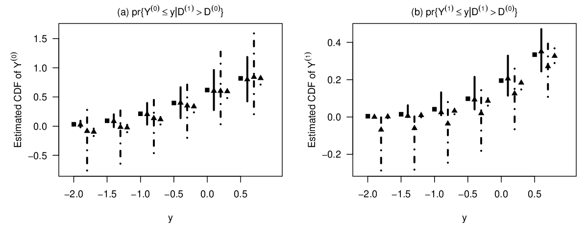
We compare the performance of our proposed Auto- $\kappa$ estimator with $\kappa$ weighting (Abadie 2003) and the original debiased machine learning with explicit propensity scores (Chernozhukov et al. 2018) in simulations. We focus on counterfactual distributions as our choice of complier parameter $\theta_{0}$ over the grid $\mathcal{U}$ specified on the horizontal axis of Figure 1.

Refer to caption — Figure 1: Numerical stability simulation. Simulation performance of $\kappa$ weight (line), debiased machine learning (dot dash), and Auto- $\kappa$ (dots) estimators for the counterfactual distribution, where the grid point is specified on the horizontal axis. The true values are solid squares. The vertical lines mark the 10% and 90% quantiles of the estimates across simulation draws and the solid triangles mark the median.

We consider a simple simulation design where $Y$ is a continuous outcome, $D$ is a binary treatment, $Z$ is a binary instrumental variable, and $X$ is a continuous covariate. We provide more details on the simulation design below. Each simulation consists of $n=1000$ observations. We conduct 1000 such simulations and implement each estimator as follows.

For the $\kappa$ weight, we estimate the propensity score $\hat{\pi}$ by logistic regression, which we then use in the weights $\hat{\kappa}^{(0)}(W),\hat{\kappa}^{(1)}(W)$ and subsequently the estimator $\hat{\theta}$ . For debiased machine learning, we use five folds. We estimate the propensity score $\hat{\pi}$ by $\ell_{1}$ regularized logistic regression, using a dictionary of basis functions $b(X)$ consisting of fourth order polynomials of $X$ . We estimate $\hat{\gamma}$ by lasso, using a dictionary of basis functions $b(Z,X)$ consisting of fourth order polynomials of $X$ and interactions between $Z$ and the polynomials.

For Auto- $\kappa$ , the key difference is that instead of estimating the propensity score, we directly estimate the balancing weight $\hat{\alpha}$ as described in Appendix A, using a dictionary of basis functions $b(Z,X)$ consisting of fourth order polynomials of $X$ and interactions between $Z$ and the polynomials. Subsequently, we estimate $\hat{\theta}$ and construct simultaneous confidence bands by steps outlined above. Since the true propensity scores $\pi_{0}(X)$ are highly nonlinear, we expect $\kappa$ weighting and debiased machine learning to encounter issues of numerical instability. Furthermore, $\kappa$ weighting might not be as efficient as the debiased machine learning and Auto- $\kappa$ estimators, which have the semiparametrically efficient asymptotic variance.

Table 2: Bias and RMSE simulation for

\text{pr}\{Y^{(0)}\leq y\mid D^{(1)}>D^{(0)}\}

	Bias			RMSE
$y$	$\kappa$ weight	DML	Auto- $\kappa$	$\kappa$ weight	DML	Auto- $\kappa$
-2.0	-3	-138	-37	99	3070	75
-1.5	-1	-119	-32	172	2576	76
-1.0	3	-45	-20	250	2040	79
-0.5	2	-35	2	384	1953	80
0.0	-17	18	21	556	1738	92
0.5	-12	3	34	638	3072	98
overall	-5	-53	-5	350	2391	83

Notes: RMSE, root mean square error; DML, debiased machine learning; Auto- $\kappa$ , automatic $\kappa$ weighting. All entries have been multiplied by $10^{3}$ .

Table 3: Bias and RMSE simulation for

\text{pr}\{Y^{(1)}\leq y\mid D^{(1)}>D^{(0)}\}

$y$	$\kappa$ weight	DML	Auto- $\kappa$	$\kappa$ weight	DML	Auto- $\kappa$
	Bias			RMSE
-2.0	2	-115	13	28	444	15
-1.5	4	-114	12	39	441	16
-1.0	8	-110	11	57	432	20
-0.5	16	-103	11	78	410	26
0.0	21	-93	16	90	379	35
0.5	21	-79	27	92	315	44
overall	12	-102	15	64	403	26

Notes: RMSE, root mean square error; DML, debiased machine learning; Auto- $\kappa$ , automatic $\kappa$ weighting. All entries have been multiplied by $10^{3}$ .

For each value in the grid $\mathcal{U}$ , Tables 2 and 3 present the bias and the root mean square error (RMSE) of each estimator across simulation draws. The last row averages the performance across grid points. Figure 1 visualizes the median as well as the 10% and 90% quantiles across simulation draws. Auto- $\kappa$ outperforms debiased machine learning by a large margin due to numerical stability. Even though Auto- $\kappa$ uses regularized machine learning to estimate $(\hat{\gamma},\hat{\alpha})$ , regularization bias does not translate into bias for estimating the counterfactual distribution due to the doubly robust moment function. In terms of efficiency, Auto- $\kappa$ substantially outperforms $\kappa$ weighting. Lastly, the simultaneous confidence bands based on the Auto- $\kappa$ estimator have coverage probability of 98.4% for the counterfactual distribution of $Y^{(0)}$ and 93.6% for the counterfactual distribution of $Y^{(1)}$ , which are quite close to the nominal level of 95%.

Numerical instability from inverting $\hat{\pi}$ is a known issue. In practice, researchers may try trimming and censoring. Trimming means excluding observations for which $\hat{\pi}$ is extreme. We trim according to Belloni et al. 2017, dropping observations with $\hat{\pi}$ not in $(10^{-12},1-10^{-12})$ . Censoring means imposing bounds on $\hat{\pi}$ for such observations. We censor by setting $\hat{\pi}<10^{-12}$ to be $10^{-12}$ and $\hat{\pi}>1-10^{-12}$ to be $1-10^{-12}$ . Auto- $\kappa$ without trimming or censoring outperforms $\kappa$ weighting and debiased machine learning even with trimming and censoring in this simulation design. Compare Figure 1, which has no preprocessing, with Figure 2, which has trimming, and Figure 3, which has censoring, to see this phenomenon. This property is convenient, since ad hoc trimming and censoring have limited theoretical justification (Crump et al. 2009).

E.3 Design

Each simulation consists of a sample of $n=1000$ observations. A given observation is generated from the following model.

1.

Draw $X$ from $\mathcal{U}[0,1]$ .
2.

Draw $Z\mid X=x$ from Bernoulli $\{\pi_{0}(x)\}$ , where $\pi_{0}(x)=(0.05)1_{x\leq 0.5}+(0.95)1_{x>0.5}.$
3.

Draw $D\mid Z=z,X=x$ from Bernoulli $(zx)$ .
4.

Draw $Y\mid Z=z,X=x$ from $\mathcal{N}(2zx^{2},1)$ .

From observations of $W=(Y,D,Z,X^{\top})^{\top}$ , we estimate complier counterfactual outcome distributions $\hat{\theta}=(\hat{\beta}^{\top},\hat{\delta}^{\top})^{\top}$ at a few grid points $y$ in $(-2.0,-1.5,-1.0,-0.5,1.0,0.5)$ . The true parameter values are

\displaystyle\beta_{0}^{y}

\displaystyle=\frac{\int_{0}^{1}\{\Phi(y-2x^{2})(x-1)+\Phi(y)\}\mathrm{d}x}{\int_{0}^{1}x\mathrm{d}x},\quad\delta_{0}^{y}=\frac{\int_{0}^{1}\{\Phi(y-2x^{2})x\}\mathrm{d}x}{\int_{0}^{1}x\mathrm{d}x}.

Appendix F Application details

Angrist and Evans 1998 estimate the impact of childbearing $D$ on female labor supply $Y$ in a sample of 394,840 mothers, aged 21–35 with at least two children, from the 1980 Census. The first instrument $Z_{1}$ is twin births: $Z_{1}$ indicates whether the mother’s second and third children were twins. The second instrument $Z_{2}$ is same-sex siblings: $Z_{2}$ indicates whether the mother’s initial two children were siblings with the same sex. The authors reason that both $(Z_{1},Z_{2})$ are quasi random events that induce having a third child such that the independence assumption holds unconditionally. However, the instruments are not independent of $X$ , and therefore $\pi_{0}(X)$ still depends on $X$ and may be estimated.

Angrist and Fernández-Val 2013 use parametric $\kappa$ weights to estimate two complier characteristics: (i) the average age of the mother’s second child; and (ii) the years of schooling of the mother. For a given characteristic $f(X)=X$ , the authors specify the instrument propensity score model as

\pi_{0}(X)=[1+\exp\{-(\beta_{0}+\beta_{1}X+\beta_{2}X^{2}+\beta_{3}X^{3}+\beta_{4}X^{4})\}]^{-1}.

As discussed in Section 3, such an approach is only valid when the parametric assumption on $\pi_{0}(X)$ is correct.

The semiparametric Auto- $\kappa$ approach we propose combines the doubly robust moment function from Theorems 1 and 2 with the meta procedure in Algorithm 2 and the regularized balancing weights in Algorithm 3. We expand the dictionary of basis functions to include sixth order polynomials of $X$ , and interactions between $Z$ and polynomials of $X$ . We directly estimate and regularize both the regression $\hat{\gamma}$ and the balancing weights $\hat{\alpha}$ , tuning the regularization according to Algorithm 4. We set the hyperparameters $(c_{1},c_{2},c_{3})$ as $(0.5,0.1,0.1)$ . In sample splitting, we partition the sample into five folds. The estimated balancing weights $\hat{\alpha}$ imply extreme twins-instrument propensity scores for a few observations. We censor the extreme propensity scores by setting the implied $\hat{\pi}<10^{-12}$ to be $10^{-12}$ and $\hat{\pi}>1-10^{-12}$ to be $1-10^{-12}$ .

Finally, as a robustness check, we verify that $\kappa$ weighting and Auto- $\kappa$ yield similar estimated shares of compliers, i.e. similar estimates of $\text{pr}\{D^{(1)}>D^{(0)}\}$ . These shares are typically reported in empirical research to interpret the strength and relevance of an instrumental variable. In the language of two stage least squares, these estimates correspond to the first stage. Table 4 reports the complier share estimates underlying the results of Table 1. Auto- $\kappa$ produces similar complier share estimates to the $\kappa$ weight approach of Angrist and Fernández-Val 2013 while allowing for more flexible models and regularization.

Table 4: Comparison of complier shares

	Average age of second child		Average schooling of mother
	Twins	Same-sex	Twins	Same-sex
$\kappa$ weight	0.60	0.06	0.60	0.06
Auto- $\kappa$	0.73	0.06	0.76	0.06

		$\displaystyle E\left[\left\|n^{-1/2}\sum_{\ell=1}^{L}\sum_{i\in I_{\ell}}-\{\hat{\alpha}_{-\ell}(Z_{i},X_{i})-\alpha_{0}(Z_{i},X_{i})\}A(\theta_{0})\{\hat{\gamma}_{-\ell}(Z_{i},X_{i})-\gamma_{0}(Z_{i},X_{i})\}\right\|\right]$
		$\displaystyle\leq\sum_{\ell=1}^{L}E\left[n^{1/2}\frac{1}{n}\sum_{i\in I_{\ell}}\left\|-\{\hat{\alpha}_{-\ell}(Z_{i},X_{i})-\alpha_{0}(Z_{i},X_{i})\}A(\theta_{0})\{\hat{\gamma}_{-\ell}(Z_{i},X_{i})-\gamma_{0}(Z_{i},X_{i})\}\right\|\right]$
		$\displaystyle=\sum_{\ell=1}^{L}E\left(E\left[n^{1/2}\frac{1}{n}\sum_{i\in I_{\ell}}\left\|\{\hat{\alpha}_{-\ell}(Z_{i},X_{i})-\alpha_{0}(Z_{i},X_{i})\}A(\theta_{0})\{\hat{\gamma}_{-\ell}(Z_{i},X_{i})-\gamma_{0}(Z_{i},X_{i})\}\right\|\mid I_{-\ell}\right]\right)$
		$\displaystyle=\sum_{\ell=1}^{L}E\left(E\left[\left\|n^{1/2}\frac{n_{\ell}}{n}\{\hat{\alpha}_{-\ell}(Z_{i},X_{i})-\alpha_{0}(Z_{i},X_{i})\}A(\theta_{0})\{\hat{\gamma}_{-\ell}(Z_{i},X_{i})-\gamma_{0}(Z_{i},X_{i})\}\right\|\mid I_{-\ell}\right]\right).$

		$\displaystyle E\left[\|n^{1/2}\frac{n_{\ell}}{n}\{\hat{\alpha}_{-\ell}(Z_{i},X_{i})-\alpha_{0}(Z_{i},X_{i})\}A(\theta_{0})\{\hat{\gamma}_{-\ell}(Z_{i},X_{i})-\gamma_{0}(Z_{i},X_{i})\}\|\mid I_{-\ell}\right]$
		$\displaystyle\leq E\left[\|n^{1/2}\{\hat{\alpha}_{-\ell}(Z_{i},X_{i})-\alpha_{0}(Z_{i},X_{i})\}A(\theta_{0})\{\hat{\gamma}_{-\ell}(Z_{i},X_{i})-\gamma_{0}(Z_{i},X_{i})\}\|\mid I_{-\ell}\right]$
		$\displaystyle\leq n^{1/2}\\|\hat{\alpha}_{-\ell}-\alpha_{0}\\|A(\theta_{0})\\|\hat{\gamma}_{-\ell}-\gamma_{0}\\|$
		$\displaystyle=o_{p}(1).$

	$\displaystyle E\left(\|\xi\|\right)$	$\displaystyle\leq E\left\{\|\hat{\gamma}_{-\ell}(1,X)-\gamma_{0}(1,X)\|\right\}$
		$\displaystyle\quad+E\left\{\|\hat{\gamma}_{-\ell}(0,X)-\gamma_{0}(0,X)\|\right\}$
		$\displaystyle\quad+E\left[\|\{\hat{\alpha}_{-\ell}(Z,X)-\alpha_{0}(Z,X)\}\{V-\gamma_{0}(Z,X)\}\|\right]$
		$\displaystyle\quad+E\left[\|\{\hat{\alpha}_{-\ell}(Z,X)-\alpha_{0}(Z,X)\}\{\gamma_{0}(Z,X)-\hat{\gamma}_{-\ell}(Z,X)\}\|\right]$
		$\displaystyle\quad+E\left[\|\alpha_{0}(Z,X)\{\gamma_{0}(Z,X)-\hat{\gamma}_{-\ell}(Z,X)\}\|\right].$

	$\displaystyle E\left\{\|\hat{\gamma}_{-\ell}(1,X)-\gamma_{0}(1,X)\|\right\}$	$\displaystyle=E\left[E\left\{\|\hat{\gamma}_{-\ell}(1,X)-\gamma_{0}(1,X)\|\mid I_{-\ell}\right\}\right]$
		$\displaystyle\leq E\{\\|\hat{\gamma}_{-\ell}(1,x)-\gamma_{0}(1,x)\\|\}$
		$\displaystyle\leq CE(\\|\hat{\gamma}_{-\ell}-\gamma_{0}\\|)$
		$\displaystyle=o_{p}(1).$

		$\displaystyle E[\|\{\hat{\alpha}_{-\ell}(Z,X)-\alpha_{0}(Z,X)\}\{V-\gamma_{0}(Z,X)\}\|]$
		$\displaystyle=E\left(E[\|\{\hat{\alpha}_{-\ell}(Z,X)-\alpha_{0}(Z,X)\}\{V-\gamma_{0}(Z,X)\}\|\mid I_{-\ell}]\right)$
		$\displaystyle\leq E\left\{\\|\hat{\alpha}_{-\ell}-\alpha_{0}\\|\\|v-\gamma_{0}(z,x)\\|\right\}$
		$\displaystyle\leq CE(\\|\hat{\alpha}_{-\ell}-\alpha_{0}\\|)$
		$\displaystyle=o_{p}(1).$

Double Robustness for Complier Parameters and a Semiparametric Test for Complier Characteristics

Abstract

1 Introduction and related work

2 Framework

Assumption 1 (Instrumental variable identification).

Definition 1 (General class of complier parameters (Abadie 2003)).

Definition 2 (Average complier characteristics).

3 Key insight

3.1 Classic approaches: Wald formula and κ\kappa weight

3.2 Doubly robust moment for a special case

3.3 A new synthesis that allows for machine learning

Proposition 1 (κ\kappa weight as balancing weight).

Proof.

Proposition 2 (Balancing weight as Riesz representer).

Proof.

4 The doubly robust moment

Theorem 1 (Cases 1 and 2).

Proof.

Theorem 2 (Case 3).

Proof.

5 A hypothesis test to compare observable characteristics

5.1 Corollaries for average complier characteristics

Corollary 1 (Average complier characteristics).

Proof.

Algorithm 1 (Hypothesis test for difference of average complier characteristics).

Corollary 2 (Hypothesis test for difference of average complier characteristics).

Proof.

5.2 Empirical application

6 Conclusion

Appendix A Automatic κ\kappa weights

A.1 Estimation

Algorithm 2 (Debiased machine learning).

Algorithm 3 (Regularized balancing weight).

A.2 Affine moments

Definition 3 (Affine moment).

Definition 4 (Empirically important complier parameters).

Corollary 3 (Empirically important parameters have affine moments).

Proof.

A.3 Inference

Assumption 2 (Regularity conditions for complier parameter estimation).

Theorem 3 (Consistency and asymptotic normality).

Proof.

References

Supplementary material

Appendix B Rate conditions

Assumption 3 (Bounded dictionary).

Assumption 4 (Dense balancing weight).

Assumption 5 (Sparse balancing weight).

Assumption 6 (Regularization).

Lemma 1 (Dense balancing weight rate).

Lemma 2 (Sparse balancing weight rate).

Assumption 7 (Regression rate).

Corollary 4 (Verifying rate condition).

Appendix C Proof of consistency and asymptotic normality for Auto-κ\kappa

C.1 Lemmas from previous work

Definition 5.

Proposition 3 (Lemma C1 of Chernozhukov et al. 2018b).

Proposition 4 (Lemma 4 of Chernozhukov et al. 2018b).

Proof of Lemma 1.

Proof of Lemma 2.

Lemma 3 (Theorem 6 of Chernozhukov et al. 2018b).

Lemma 4.

Proof.

Lemma 5 (Theorem 2.1 Newey and McFadden 1994).

C.2 Consistency and asymptotic normality

Proposition 5.

Proof.

Proposition 6.

Proof.

Proposition 7.

Proof.

Proposition 8.

Proof.

Proposition 9.

Proof.

Proposition 10.

Proof.

Proof of Theorem 3.

Appendix D Tuning

Algorithm 4 (Regularized balancing weight with tuning).

3.1 Classic approaches: Wald formula and $\kappa$ weight

Proposition 1 ( $\kappa$ weight as balancing weight).

Appendix A Automatic $\kappa$ weights

Appendix C Proof of consistency and asymptotic normality for Auto- $\kappa$