On the natural gradient for variational quantum eigensolver

The field of quantum computing is still far away from the stage where ideal fault-tolerant systems are available. Hence a recent trend is to seek the potential of quantum-classical hybrid algorithms which might have some advantages over purely classical computers. The variational method is one such approach; particularly the variational quantum eigensolver (VQE) O'Brien 2014; McClean 2016; Kandala 2017; Temme 2017; AdptVQE 2019; Fujii 2019 is a hybrid algorithm using a parametrized quantum computer to drive the quantum state and a classical computer for optimizing those parameters, for finding the ground state of a given Hamiltonian.

It is clear that the performance of VQE heavily depends on the classical optimization part. In fact various types of optimizers have been tested, such as the ordinary gradient and simultaneous perturbation stochastic approximation SPSA. On the other hand, the so-called natural gradient optimization method Amari 1998 is often used in the classical literature, particularly for machine learning problems. Actually the natural gradient is the optimizer that takes into account the geometric structure of the parameter space, which is usually very complicated, e.g., in the case of large neural networks, and hence it often works very well without being trapped in local minimums or plateaus in the parameter space.

Interestingly, it is known in the literature (see e.g., Carleo 2017; Cirac 2018) that, in the case when the quantum Fubini-Study metric is taken to measure the geometric structure, the VQE algorithm with the natural gradient is equivalent to the stochastic reconfiguration Sorella 2001; Sorella 2004 and the imaginary time evolution (ITE) Benjamin 2018a; Benjamin 2018b (a certain correction term might be necessary). With this background, very recently, Stokes et al. Carleo 2019 developed the general framework for applying the natural gradient for variational quantum problems and demonstrated that it actually works for a particular VQE problem better than some standard optimizers; in particular, they gave an efficient algorithm for computing the Fubini-Study metric in each iteration step of the VQE procedure.

The aim of this paper is, with detailed investigations for some simple VQE problems, to show how the natural gradient makes use of the geometric property of the parametrized quantum state to realize a better optimization process of the parameters, and accordingly to give a suggestion about in what situation the natural gradient method should be used in VQE problems.

The basic procedure of VQE is, given a (short) quantum circuit $U(\theta)$ with parameters $\theta=(\theta_{1},\ldots,\theta_{m})$, to repeatedly update $\theta$ so that the mean energy $f(\theta)=\langle{\phi(\theta)}|H|{\phi(\theta)}\rangle$ decreases toward its minimum for the ansatz $|{\phi(\theta)}\rangle=U(\theta)|{0}\rangle$ with $|{0}\rangle$ the initial state; hence VQE is a hybrid algorithm composed of the quantum computing, which generates a quantum state possibly hard to classically simulate, and the classical computing, which iterates the optimization process of the parameters. A simple optimizer is the ordinary gradient descent:

where $\theta_{k}$ is the parameter at the $k$th step, $\eta_{k}$ is the coefficient, and $\partial f(\theta)/\partial\theta$ is the gradient vector of $f(\theta)$.

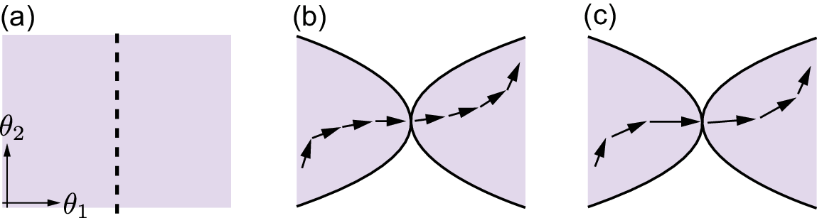
Now note that the dynamics (1) assumes that the parameter space is a flat Euclidean space. However, as will be demonstrated, the actual parameter space is not flat in the sense of indistinguishability. For instance, for the two-parameters case $f(\theta)=f(\theta_{1},\theta_{2})$, there might be a point $\theta_{1}=\bar{\theta}_{1}$ such that $f(\bar{\theta}_{1},\theta_{2})$ takes the same value for all $\theta_{2}$; in this case, because any two different $\theta_{2}$ cannot be distinguished, this 1-dimensional set of parameters (the dotted line in Fig. 1(a)) must be regarded as a singular point in the parameter space. Consequently, the parameter space must be a non-Euclidean one as shown in Fig. 1(b). Around the singular point, roughly speaking the volume of metric becomes small, and thus the dynamics of parameters should be modified, taking into account this geometry; the natural gradient does this, by stretching the gradient vector as shown in Fig. 1(c) while the ordinary one (1) does not. As consequence, the natural gradient drives the parameter point faster than the ordinary one, especially around the singular points. Mathematically, the natural gradient optimizer updates the parameters according to

where $F(\theta)$ is the Riemannian metric matrix at $\theta$. In fact, $F^{-1}\partial f/\partial\theta$ is the steepest descent vector in this Riemanean space.

In the VQE setting, the metric can be induced from the indistinguishability of the function $f(\theta)=\langle{\phi(\theta)}|H|{\phi(\theta)}\rangle$. The most “detailed” distinguishing way is to measure the distance in the space of pure quantum states; actually if $|{\phi(\theta_{A})}\rangle=|{\phi(\theta_{B})}\rangle$, then $f(\theta_{A})=f(\theta_{B})$. Typically the Fubini-Study distance is used for this purpose, the infinitesimal version of which is given by

where $F=(F_{ij})$ is the Fubini-Study (or more generally the quantum Fisher information) metric:

Here $|{\partial_{i}\phi}\rangle=\partial|{\phi(\theta)}\rangle/\partial\theta_{i}$ denotes the partial derivative of $|{\phi(\theta)}\rangle$ with respect to $\theta_{i}$. The singular point is now clearly characterized by the point where the matrix $F$ is not of full-rank.

We can introduce another measure for indistinguishability; the energy function is now represented in terms of the classical probability distribution $p(\theta)=\{p_{i}(\theta)\}$ as

where $\lambda_{i}$ and $E_{i}$ are the eigenvalue and the corresponding projection operator of $H$, respectively. Clearly, if $p(\theta_{A})=p(\theta_{B})$, then $f(\theta_{A})=f(\theta_{B})$. Typically the distance of probability distributions is measured by the Kullback-Leibler divergence, the infinitesimal version of which is given by

where $F^{C}=(F^{C}_{ij})$ is the Fisher information metric:

As in Ref. Carleo 2019, this paper studies the natural gradient with the quantum metric (3); using Eq. (4) is an interesting direction, but only a small comment will be given in the next section.

Lastly let us review the theory of ITE Benjamin 2018a. The basic idea is to project the energy-decreasing (hence non-Unitary) dynamics $d|{\psi}\rangle/dt=-(H-\langle{\psi}|H|{\psi}\rangle)|{\psi}\rangle$ to the ansatz space; in the discrete time representation the following parameter update rule governs the projected dynamics:

where $A_{ij}={\rm Re}(\langle{\partial_{i}\phi}|{\partial_{j}\phi}\rangle)$. Therefore by adding the second term in Eq. (3) to $A_{ij}$, we find that the ITE is equivalent to the natural gradient. Although a different projection method leads to the ansatz dynamics of ITE which is completely equivalent to the natural gradient, as shown in Benjamin 2018b; Carleo 2019, in this paper let us call Eq. (5) the ITE. Also note that the residual matrix $(A-F)_{ij}=\langle{\partial_{i}\phi}|{\phi}\rangle\langle{\phi}|{\partial_{j}\phi}\rangle$ is positive semidefinite, meaning that $A\geq F$ holds in the sense of matrix inequality. Hence together with the well-known fact that the quantum Fisher information is the supremum of all the induced classical Fisher information Caves 1994, we now have

where the existence of $(F^{C})^{-1}$ is assumed. This general inequality indicates that ITE does not so much care the metric; hence if $F$ or $F^{C}$ stretches the gradient vector too much, which is problematic at around the target point, then switching the strategy to ITE or the ordinary gradient would be recommended.

Let us begin with the single qubit case. The goal is to drive the ansatz state

to the ground state of the Hamiltonian $H=\sigma_{x}$. It is clear that the north pole ($\theta_{1}=0$) and the south pole ($\theta_{1}=\pi/2$) in the Bloch sphere are singular points, where $|{\phi(\theta)}\rangle$ does not depend on $\theta_{2}$. Now the Fubini-Study metric (3) is calculated as

The two singular points are correctly characterized by the points such that ${\rm det}(F)=0$. On the other hand the matrix in ITE (5) is

which does not capture the singularity of $|{\phi(\theta)}\rangle$ at $\theta_{1}=\pi/2$. The energy function is $f(\theta)=\langle{\phi(\theta)}|H|{\phi(\theta)}\rangle=\sin(2\theta_{1})\cos(2\theta_{2})$. The gradient vector of $f(\theta)$ is obtained as

All the numerical simulation shown below are based on the above analytic expressions, and no approximation is made. Also $\eta_{k}$ is fixed to $\eta_{k}=0.05$ for all $k$.

First let us see the case where the initial point of parameters is given by $P_{0}=(\theta_{1},\theta_{2})=(\pi/12,\pi/12)$. The point of this choice is as follows; now $P_{*}=(\theta_{1},\theta_{2})=(-\pi/4,0)$ is the optimum point closest to $P_{0}$ and $\tilde{P}_{*}=(\theta_{1},\theta_{2})=(\pi/4,\pi/2)$ is the second-closest optimum point in the Euclidean metric; however, now the line $\theta_{1}=0$ constitutes a singular point, and those distances might change depending on the metric because the path from $P_{0}$ to $P_{*}$ must cross this point while the path from $P_{0}$ to $\tilde{P}_{*}$ does not. In fact, as shown in Fig. 2, the natural gradient and ITE find $\tilde{P}_{*}$ as the closest target. As a result, the natural gradient and ITE realize faster convergence to the ground state compared to the ordinary method.

Next let us see the case where the initial point is given by $(\theta_{1},\theta_{2})=(5\pi/12,\pi/12)$. Note that in this case there is a singular point corresponding to $\theta_{1}=\pi/2$ near the initial point, but this singularity is recognized only by the natural gradient. Then, as shown in Fig. 3, the ordinary gradient and ITE find $(\theta_{1},\theta_{2})=(3\pi/4,0)$ as the closest optimum point, while the natural one takes the path toward $\tilde{P}_{*}$ according to the metric. Consequently, the natural gradient reaches the ground state first. Therefore we can conclude that the natural gradient actually makes use of the geometry of parameter space and realizes the fast convergence to the target ground state.

Lastly let us discuss the case using the classical Fisher metric (4) induced from the measurement of $H$ for the natural gradient method. Now the outcome is $h_{+1}=+1$ with probability $p_{+}(\theta)=|\langle{x+}|{\phi(\theta)}\rangle|^{2}=(1+\sin(2\theta_{1})\cos(2\theta_{2}))/2$ or $h_{-1}=-1$ with probability $p_{-}(\theta)=1-p_{+}(\theta)$. That is, our classical probability distribution is the Bernoulli one $p(\theta)=\{p_{+}(\theta),~p_{-}(\theta)\}$. The $2\times 2$ Fisher information matrix is then given by

which is clearly of rank-1, without respect to the form of $p_{+}(\theta_{1},\theta_{2})$. This means that the whole 2-dimensional parameter space is singular, and the natural gradient cannot be directly applied. However, because $F^{C}$ depends on $H$ whereas $F$ does not, the natural gradient for VQE with the classical Fisher information might be effectively applied to a complicated Hamiltonian.

The second case-study is on the problem of finding the ground state of the ${\rm}H_{2}$ molecule; the Hamiltonian can be reduced and modeled using two qubits as Temme 2017

where $\alpha=0.4$ and $\beta=0.2$. This has four eigenvalues

and particularly the minimum eigenvector, i.e., the ground state, is given by

The ansatz is taken as

where $U_{\rm ent}=|{0}\rangle\langle{0}|\otimes I+|{1}\rangle\langle{1}|\otimes\sigma_{x}$ denotes the CNOT gate and $R_{y}(\theta)$ denotes the single-qubit rotation operator defined by

This is a typical hardware-efficient ansatz, illustrated in Fig. 4.

The Fubini-Study metric (3) is calculated as

Note that $|{\phi(\theta)}\rangle$ is a real vector and thus $\langle{\partial_{i}\phi}|{\phi}\rangle=0$ for all $i$. Hence $F=A$; that is, ITE is equivalent to the natural gradient. Now the determinant of $F$ is given by

The parameters satisfying ${\rm det}(F)=0$ constitute the set of singular points, which has a clear physical meaning as follows. In general, the entanglement of the bipartite state $|{\Psi}\rangle$ can be quantified by the entanglement entropy

In our case, it is given by

where

Hence, $S(|{\phi}\rangle)=0$ if and only if ${\rm det}(F)=0$. That is, the set of singular points represents the set of all separable states. This makes sense, because if the state $U_{\rm ent}(R_{y}(2\theta_{1})\otimes R_{y}(2\theta_{2}))|{0}\rangle\otimes|{0}\rangle$ is separable, then the local operation $R_{y}(2\theta_{3})\otimes R_{y}(2\theta_{4})$ can never entangle this state for any parameter choice.

Let us now see the results of numerical simulation. Again the learning coefficient is fixed to $\eta_{k}=0.05$ for all $k$. First, Fig. 5 shows the trajectory of the parameter dynamics (Top) and the change of $f(\theta)$ over the VQE iteration step, for the case where the initial point is $(\theta_{1},\theta_{2},\theta_{3},\theta_{4})=(-0.2,-0.2,0,0)$. As shown in the figure, the natural gradient achieves the faster convergence to the minimum energy $h_{4}\approx-0.82$ than the ordinary gradient. This faster convergence might be explained as follows. If the initial value of $\theta_{3}$ and $\theta_{4}$ are chosen as $(\theta_{3},\theta_{4})=(0,0)$, the initial state is

Hence, if $\theta_{2}$ is nearly zero, the initial state is already close to the target ground state (8), meaning that $(\theta_{2},\theta_{3},\theta_{4})$ need not be largely changed. It seems that the natural gradient effectively utilizes this fact, as seen in Fig. 5.

Next let us see the case where the initial value of parameters are $(\theta_{2},\theta_{3},\theta_{4})=(\pi/2,0,0)$; in this case, the initial state (9) is $|{\phi}\rangle=[0,\cos\theta_{1},\sin\theta_{1},0]^{\top}$, which is thus close to the first or second excited state $(|{0,1}\rangle\pm|{1,0}\rangle)/\sqrt{2}$. Hence the parameters have to be largely changed to transfer the initial state to the target ground state. Then there might be some singular points along this passage; the natural gradient may have an advantage in such a case, by stretching the gradient vector depending on the metric, as explained in Fig. 1. Figure 6 plots the energy with the initial value $\theta_{1}=7\pi/32$, which indeed demonstrates this desirable scenario; that is, at around the first excited state with energy $-\beta=-0.2$, the natural gradient can efficiently search the path to get out the plateau and move toward the ground state faster than the ordinary gradient. Note that during the second drop-off, the natural gradient experiences a steep rise in energy, meaning that actually the path in the parameter space moves near a singular point such that $F^{-1}$ takes a large value. Such a sudden change of the parameters can be avoided by adding a small positive number to the eigenvalues of $F$ via the singular value decomposition of $F$.

Lastly we discuss the toy molecule having Hamiltonian (7) with $\alpha=0.4$ and $\beta=0.02$. In this case, the target ground state (8) is close to the separable state $|{1,1}\rangle$ with minimum energy $h_{4}\approx-2\alpha=-0.8$. This should be problematic for the natural gradient, because, as seen above, all the separable states correspond to the singular points in the parameter space; as a result, in this case the natural gradient vector must be largely stretched near the target ground state. This is actually seen in Fig. 7, showing that the state with natural gradient never stay at the ground state. In such a case the learning coefficient $\eta_{k}$ should be modified to monotonically decrease, e.g., $\eta_{k}=1/k$; but this strategy did not work well for this problem. Hence what we have learned from this case-study on the use of natural gradient is that the metric should be carefully analyzed so that the target state (which is however unknown) would not lie near singular points in the parameter space.

Some case-studies on the natural gradient for the VQE problems have been discussed in this paper. It is hoped that the reader would gain some insight about how to make use of the geometric property of a parametrized ansatz state to effectively apply the natural gradient method, possibly even to a relatively large VQE problem.

This work was supported by MEXT Quantum Leap Flagship Program Grant Number JPMXS0118067285. The author acknowledges helpful discussion with Y. Onishi and Y. Yamaji.

References

- (1) A. Peruzzo, J. McClean, P. Shadbolt, M. Yung, X. Zhou, P. J. Love, A. Aspuru-Guzik, and J. L. O’Brien, A variational eigenvalue solver on a photonic quantum processor, Nat. Commun. 5, 4213 (2014).
- (2) J. R. McClean, J. Romero, R. Babbush, and A. Aspuru-Guzik, The theory of variational hybrid quantum-classical algorithms, New J. Phys. 18, 023023 (2016).
- (3) A. Kandala, A. Mezzacapo, K. Temme, M. Takita, M. Brink, J. M. Chow, and J. M. Gambetta, Hardware-efficient variational quantum eigensolver for small molecules and quantum magnets, Nature 549, 242 (2017).
- (4) S. Bravyi, J. M. Gambetta, A. Mezzacapo, and K. Temme, Tapering off qubits to simulate fermionic Hamiltonians, arXiv:1701.08213 (2017).
- (5) H. R. Grimsley, S. E. Economou, E. Barnes, and N. J. Mayhall, An adaptive variational algorithm for exact molecular simulations on a quantum computer, Nat. Commun. 10, 3007 (2019).
- (6) N. Yoshioka, Y. O. Nakagawa, K. Mitarai, and K. Fujii, Variational quantum algorithm for non-equilibrium steady states, arXiv:1908.09836 (2019).
- (7) J. C. Spall, Multivariate stochastic approximation using a simultaneous perturbation gradient approximation, IEEE Trans. Autom. Contr. 37, 332-341 (1992).
- (8) S. Amari, Natural gradient works efficiently in learning, Neural Computation, 10, 251/276 (1998).
- (9) G. Carleo and M. Troyer, Solving the quantum many-body problem with artificial neural networks, Science 355, 602 (2017).
- (10) I. Glasser, N. Pancotti, M. August, I. D. Rodriguez, and J. I. Cirac, Neural-network quantum states, string-bond states, and Chiral topological states, Phys. Rev. X 8, 011006 (2018).
- (11) S. Sorella. Generalized Lanczos algorithm for variational quantum Monte Carlo, Phys. Rev. B 64, 024512 (2001).
- (12) M. Casula C. Attaccalite, and S. Sorella. Correlated geminal wave function for molecules: An efficient resonating valence bond approach. Journal. Chem. Phys. 121, 7110 (2004).
- (13) S. McArdle, T. Jones, S. Endo, Y. Li, S. Benjamin, and X. Yuan, Variational quantum simulation of imaginary time evolution, arXiv:1804.03023 (2018).
- (14) X. Yuan, S. Endo, Q. Zhao, S. Benjamin, and Y. Li, Theory of variational quantum simulation, arXiv:1812.08767 (2018).
- (15) J. Stokes, J. Izaac, N. Killoran, and G. Carleo, Quantum natural gradient, arXiv:1909.02108 (2019).
- (16) S. L. Braunstein and C. M. Caves, Statistical distance and the geometry of quantum states, Phys. Rev. Lett. 72, 3439 (1994).