Temporally Grounding Language Queries in Videos by
Contextual Boundary-aware Prediction
Abstract
The task of temporally grounding language queries in videos is to temporally localize the best matched video segment corresponding to a given language (sentence). It requires certain models to simultaneously perform visual and linguistic understandings. Previous work predominantly ignores the precision of segment localization. Sliding window based methods use predefined search window sizes, which suffer from redundant computation, while existing anchor-based approaches fail to yield precise localization. We address this issue by proposing an end-to-end boundary-aware model, which uses a lightweight branch to predict semantic boundaries corresponding to the given linguistic information. To better detect semantic boundaries, we propose to aggregate contextual information by explicitly modeling the relationship between the current element and its neighbors. The most confident segments are subsequently selected based on both anchor and boundary predictions at the testing stage. The proposed model, dubbed Contextual Boundary-aware Prediction (CBP), outperforms its competitors with a clear margin on three public datasets. All codes are available on https://github.com/JaywongWang/CBP.
1 Introduction
Videos are increasingly popular in the social network. As most videos contain both activities of interest and complicated background content, temporal activity localization is of key importance for video analysis. Recently, the task of temporally grounding language queries in videos has been attracting research interest from the vision community [\citeauthoryearGao et al.2017, \citeauthoryearHendricks et al.2017]. The task aims to localize the activity of interest corresponding to a language query. This task is challenging because both videos and sentences need to be deeply incorporated to differentiate fine-grained details of different video segments and to perform segment localization. In this paper, we identify and tackle the main challenge on this task, namely, how to improve the localization precision of the desired segment given a language query.

Prior work predominantly ignores the precision of segment boundaries. Sliding window based methods scan the video by predefined windows of different sizes [\citeauthoryearGao et al.2017, \citeauthoryearHendricks et al.2017, \citeauthoryearLiu et al.2018c, \citeauthoryearWu and Han2018, \citeauthoryearLiu et al.2018b, \citeauthoryearGe et al.2019, \citeauthoryearXu et al.2019]. Because the desired segments are of varied durations, these methods cannot guarantee the complete coverage of all segments, and thus tend to produce inaccurate temporal boundaries. Other research tried to avoid this problem by designing single-stream models [\citeauthoryearBuch et al.2017, \citeauthoryearChen et al.2018] using LSTMs. Although LSTMs effectively aggregate video information, the thresholding of positive and negative samples loses boundary information. As shown in Figure 1 (b), segments overlapped with the ground truth more than a predefined threshold (e.g., 0.5) are all labeled as positive samples during training stage. Therefore, the model could be confused to localize the best matched segment at prediction. A complementary approach to improve the precision of localization is to add a location offset regression branch to the anchor-based approaches [\citeauthoryearGao et al.2017, \citeauthoryearXu et al.2019, \citeauthoryearGe et al.2019, \citeauthoryearLiu et al.2018b]. However, the added offset regression could fail when the model is unable to localize the best anchor, since the calculated offsets need to be added to the predicted anchor to generate final grounding time stamp (See Table 2 for comparison).
To improve temporal grounding precision, we propose a novel model that jointly predicts temporal anchors and boundaries at each time step, with a small computation overhead. At prediction stage, the anchors are modulated by boundary scores to generate boundary-aware grounding results. To detect semantic boundaries more accurately, contextual information is adaptively integrated into our architecture. As shown in Figure 1, the activity “fly down the mountain” exhibits different visual appearance compared to the background content. The activity is better localized with the aid of its surrounding information. To this end, we propose a self attention based contextual integration module, which is deeply embedded into the architecture. Different from [\citeauthoryearGao et al.2017, \citeauthoryearHendricks et al.2017, \citeauthoryearWu and Han2018, \citeauthoryearGe et al.2019] where context information is simply integrated by feature concatenation, we explicitly measure the different “contributions” by leveraging the self-attention technique. Noticeably, our proposed context module operates on the layer which already integrates query and video information. It thus enables our network to “perceive” the surrounding predictions and collect reliable contextual evidences before making predictions at the current step. This is different from previous context modeling, which only considers visual context but ignores the impact of language integration. Although LSTMs are also capable of summarizing contextual information, it suffers from the so-called “gradient vanishing/exploding” problem and could fail to memorize information for long segments. The proposed contextual model, however, shortens the path for remote elements and effectively aggregates useful contexts in the video.
To summarize, our main contributions are two-folds. First, we address the problem of temporally grounding language queries in videos with a simple yet effective boundary-aware approach, which effectively improves grounding precision in an end-to-end manner. Second, to better detect semantic boundaries, a self attention based module is designed to collect contextual clues. Based on interaction output of both language and video, it explicitly measures the contributions from different contextual elements. Our proposed contextual boundary-aware model (named as CBP) achieves compelling performance on three public datasets.
2 Related Work
The interdisciplinary research topics of vision and language have long been explored. Among them we emphasize the following two most relevant topics to our paper: grounding language queries in images, and grounding language queries in videos.
2.1 Grounding Language Queries in Images
Grounding language queries in images, also known as “grounding referring expressions in images”, is to spatially localize the image region corresponding to a given language query. Most work follows the standard pipeline, which first generates candidate image regions using image proposal method like [\citeauthoryearRen et al.2015], then finds the matched one to the given query. In [\citeauthoryearMao et al.2016, \citeauthoryearHu et al.2016, \citeauthoryearRohrbach et al.2016], the target image regions were extracted based on description reconstruction error or probabilities. Some studies consider incorporating contextual information into the retrieval model [\citeauthoryearHu et al.2016, \citeauthoryearYu et al.2016, \citeauthoryearChen, Kovvuri, and Nevatia2017, \citeauthoryearChen et al.2017, \citeauthoryearZhang, Niu, and Chang2018]. These “contexts” include global contexts [\citeauthoryearHu et al.2016], and contexts from other candidate regions [\citeauthoryearYu et al.2016, \citeauthoryearChen et al.2017, \citeauthoryearChen, Kovvuri, and Nevatia2017, \citeauthoryearZhang, Niu, and Chang2018]. [\citeauthoryearWang et al.2016] explored not only region-phrase relationship, but also modeled region-region and phrase-phrase structures. Some other methods exploit attention modeling in queries, images, or object proposals [\citeauthoryearEndo et al.2017, \citeauthoryearYu et al.2018, \citeauthoryearDeng et al.2018].
2.2 Grounding Language Queries in Videos
Temporally video grounding aims at extracting the corresponding video segment to a given language query. Early studies focus on constrained scenarios such as autonomous driving [\citeauthoryearLin et al.2014], or constrained setting such as alignment of multiple sentences [\citeauthoryearBojanowski et al.2015]. Recently, [\citeauthoryearGao et al.2017] and [\citeauthoryearHendricks et al.2017] extended the task to more general scenarios. [\citeauthoryearGao et al.2017] proposed to jointly model video clips and text queries using multi-modal operations, then alignment scores and location offsets were predicted based on the multi-model representation. [\citeauthoryearHendricks et al.2017] proposed to embed both modalities into a common space and minimize the squared distances. Both [\citeauthoryearGao et al.2017] and [\citeauthoryearHendricks et al.2017] exploited temporal visual contexts for localization. [\citeauthoryearWu and Han2018] integrated multiple interactions between different modalities and proposed Multi-modal Circulant Fusion. [\citeauthoryearLiu et al.2018b] designed a memory attention network to enhance the visual features. To avoid redundant computation caused by sliding windows, [\citeauthoryearChen et al.2018] dynamically matches language and video, and generates grounding results in one single pass. [\citeauthoryearLiu et al.2018a] designed a temporal modular network that can exploit underlying language structure. [\citeauthoryearGe et al.2019] proposed to mine semantic activity concepts to enhance the temporal grounding task. [\citeauthoryearXu et al.2019] followed a two-stage pipeline to retrieve video clips. They first generated query-specific proposals from the videos, then leveraged caption reconstruction for training. In [\citeauthoryearChen and Jiang2019], a visual concept based approach was proposed to generate proposals, followed by proposal evaluation and refinement. [\citeauthoryearWang, Huang, and Wang2019, \citeauthoryearHahn et al.2019] explored reinforcement learning to find the corresponding segments to language queries.
3 Proposed Method
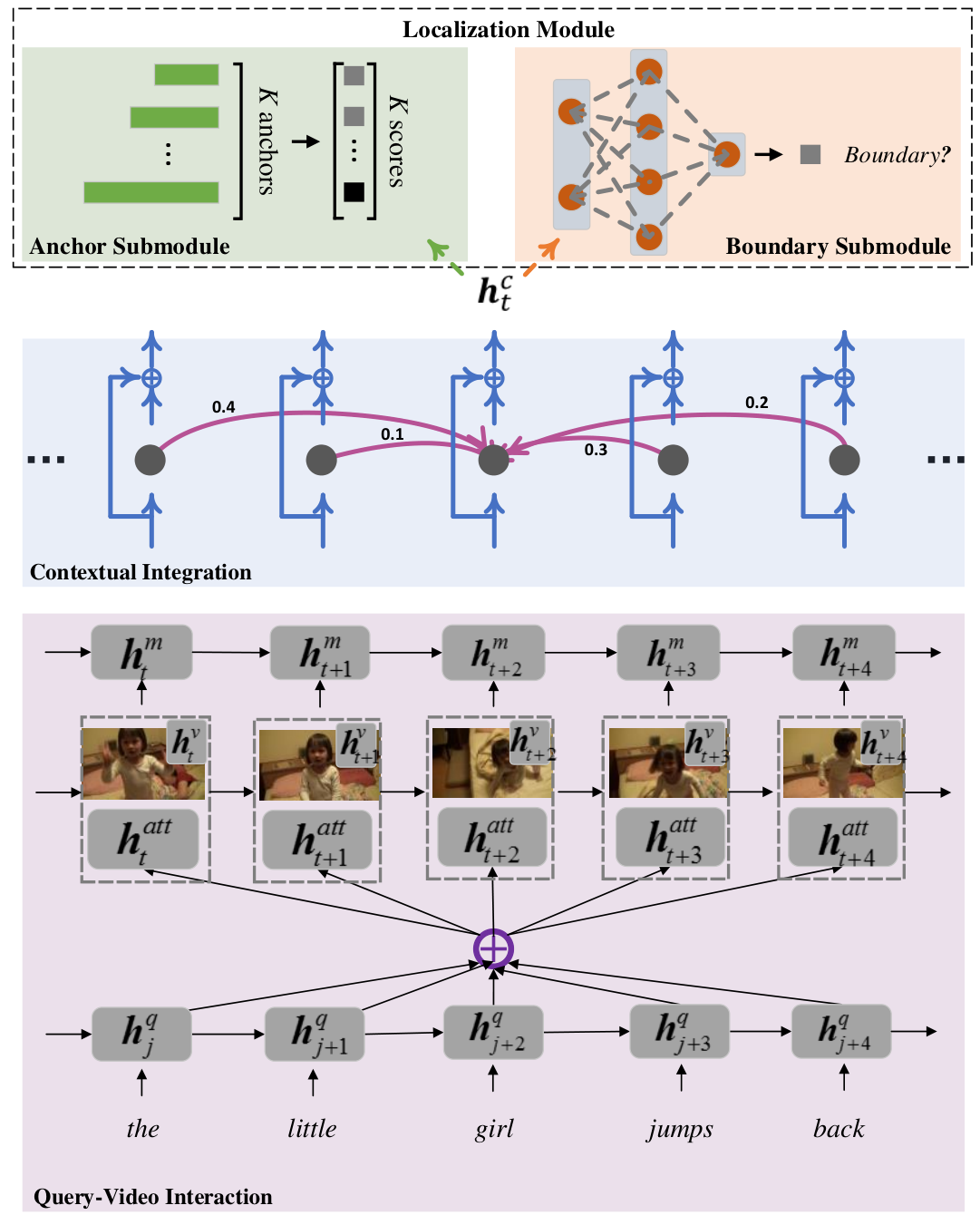
In this section we introduce our main framework for temporally grounding queries in videos, as shown in Figure 2. Our model consists of three main components: the query-video interaction module, the contextual integration module, and the localization module. The three components are deeply integrated and thus enable end-to-end training.
3.1 Problem Formulation
We denote a video as a sequence of frames . Each video is associated with a set of annotations: , where , , denote the query sentence, the start and end time of the annotated segment, respectively. Given the input video and the sentence query, our task is to localize the target segment. Each video is represented as a sequence of features . The sentence query is represented by .
3.2 Query-Video Interaction Module
Intrinsically both videos and sentence queries are sequential signals. We incorporate Match-LSTM [\citeauthoryearWang and Jiang2016, \citeauthoryearChen et al.2018] as our backbone network to learn vision-language interaction. The Match-LSTM composes of three LSTM [\citeauthoryearHochreiter and Schmidhuber] layers. The first LSTM incorporates textual information (denoted as “query LSTM”). The second LSTM encodes video motion and long-term dependencies from the input video (denoted as “video LSTM”). The third LSTM is responsible for summarizing video and language elements (denoted as “interaction LSTM”). The output states of the three LSTMs are , , and , respectively.
As shown in Figure 2, each video frame is attentively matched to different words from a query:
| (1) | ||||
| (2) | ||||
| (3) | ||||
| (4) |
where is the attended query vector, which relies on current video LSTM state and interaction LSTM state. The attended query vector is concatenated (“”) with the video state () to serve as input to the interaction LSTM to obtain next state .
By the above integration, we deeply summarize and integrate the query and the video.
3.3 Contextual Integration Module
To better capture the boundary information corresponding to the starting or ending of an activity, we explore contextual integration by leveraging the self attention technique [\citeauthoryearVaswani et al.2017] on top of the Match-LSTM. Different from pure visual contextual integration [\citeauthoryearGao et al.2017, \citeauthoryearHendricks et al.2017, \citeauthoryearHendricks et al.2018, \citeauthoryearGe et al.2019, \citeauthoryearWu and Han2018], our contextual integration module can strengthen and collect useful grounding clues as it operates on the layer which already integrates query and video information. We also explicitly model the different contributions from different “contexts” by assigning them with different attention weights. Formally, the input sequence to the contextual integration module is: , where . Since every pair from needs to be matched, we use scaled dot-product operation to perform self attention as it enjoys high computational efficiency. The relevance matrix for is:
| (5) |
where the projection matrices and . In practice, we keep by sharing projection weights at training. We find it helps improve the performance. The relevance matrix is then normalized to obtain the context weights :
| (6) |
We summarize contextual elements using the learnt attention to obtain:
| (7) |
To avoid corrupting temporal dependency of LSTM, and are integrated by concatenation operation:
| (8) |
is expected to strengthen reliable contextual evidence for localization. The operation faithfully preserves the temporal dependency of LSTM, which benefits the following prediction procedure.
3.4 Localization Module
The traditional anchor prediction focus more on coarse localization by recognizing segment content. We further propose to strengthen fine-grained semantic boundary information with an additional boundary module. The two modules share the common base network and could benefit each other at the training stage.
Anchor Submodule. We adopts similar idea as Buch et al. [\citeauthoryearBuch et al.2017]. We design anchors to match different temporal durations. Each in aggregates historical video information from position 0 to position , after query-video integration. Each hidden state will be fed into independent binary classifiers and produces confidence scores indicating the probabilities of segments specified by . denotes a video clip with end time as and start time as , where is the lengths of the predefined anchors. The segment scores are calculated by:
| (9) |
where denotes sigmoid nonlinearity. , are shared across all time steps.
Boundary Submodule. Except for the anchor prediction, we also design a parallel branch to predict boundaries of segments. The idea of boundary modeling is simple. We take as an indication of whether there is a semantic boundary at position . Specifically, a binary classifier is trained with as input. The output boundary score for current position is:
| (10) |
which measures how confident the LSTM is going through a semantic boundary. Intuitively, by comparing with its memory (historical video information), the LSTM decides whether the current step is a semantic boundary corresponding the start/end time of an activity (annotated segment).
3.5 Training
There are two main losses corresponding to the above two output modules.
Anchor Loss. Following [\citeauthoryearBuch et al.2017], the anchor labels (-dim 0-1 vector) at time step is determined by overlap threshold . We adopt weighted multi-label cross entropy as anchor loss . For a video at time :
| (11) |
where , are determined based on the numbers of positive and negative samples.
Boundary Loss. Assume the training sample is associated with ground truth boundary labels . The boundary loss is given by:
| (12) |
where is the boundary prediction score at temporal position , and are positive/negative weights.
Joint Training. We balance the anchor loss and the boundary loss by:
| (13) |
is determined by cross validation to balance the two loss terms. The CBP network can be trained in an end-to-end manner by minimizing the total loss .
3.6 Boundary-modulated Anchor Prediction
At inference stage, we calculate anchor scores and boundary scores for each video temporal location .

Local Boundary Score Fusion. As illustrated in Section 1, the anchor module cannot well reflect boundary information and can produce high scores for many segments that have overlap with the ground truth segment. To precisely localize the target segment, we first apply local score fusion to combine both anchor scores and boundary scores at temporal location . The new scores for the -th anchor at time step is:
| (14) |
where . By Equation (14), we obtain new scores at each time step . As illustrated in Figure 3, we adjust the score of each anchor by taking its start boundary and end boundary into consideration.
Global Score Ranking. The final segment scores for a video are . candidate segments with highest scores are selected and NMS (Non-Maximum Suppression) is performed to further remove redundant candidates. Please note that NMS does not affect top-1 result.
| Method | R@1 | R@1 | R@1 | R@5 | R@5 | R@5 | mIoU |
|---|---|---|---|---|---|---|---|
| IoU=0.7 | IoU=0.5 | IoU=0.3 | IoU=0.7 | IoU=0.5 | IoU=0.3 | ||
| Random Anchor | 0.22 | 0.56 | 2.23 | 1.10 | 3.55 | 9.77 | 1.89 |
| VSA-RNN [\citeauthoryearKarpathy and Fei-Fei2015] | - | 4.78 | 6.91 | - | 9.10 | 13.90 | - |
| VSA-STV [\citeauthoryearKarpathy and Fei-Fei2015] | - | 7.56 | 10.77 | - | 15.50 | 23.92 | - |
| CTRL [\citeauthoryearGao et al.2017] | 6.96 | 13.30 | 18.32 | 15.33 | 25.42 | 36.69 | 11.98 |
| MCF [\citeauthoryearWu and Han2018] | - | 12.53 | 18.64 | - | 24.73 | 37.13 | - |
| ACRN [\citeauthoryearLiu et al.2018b] | - | 14.62 | 19.52 | - | 24.88 | 34.97 | - |
| TGN [\citeauthoryearChen et al.2018] | 11.88 | 18.90 | 21.77 | 15.26 | 31.02 | 39.06 | 17.93 |
| SM-RL [\citeauthoryearWang, Huang, and Wang2019] | - | 15.95 | 20.25 | - | 27.84 | 38.47 | - |
| TripNet [\citeauthoryearHahn et al.2019] | 9.52 | 19.17 | 23.95 | - | - | - | - |
| SAP [\citeauthoryearChen and Jiang2019] | - | 18.24 | - | - | 28.11 | - | - |
| ACL [\citeauthoryearGe et al.2019] | - | 20.01 | 24.17 | - | 30.66 | 42.15 | - |
| CBP (ours) | 19.10 | 24.79 | 27.31 | 25.59 | 37.40 | 43.64 | 21.59 |
| Method | R@1 | R@1 | R@1 | R@5 | R@5 | R@5 | mIoU |
| IoU=0.7 | IoU=0.5 | IoU=0.3 | IoU=0.7 | IoU=0.5 | IoU=0.3 | ||
| CBP baseline [\citeauthoryearChen et al.2018] | 11.88 | 20.21 | 25.13 | 15.26 | 30.86 | 38.80 | 17.93 |
| + Boundary | 16.02 | 22.26 | 25.52 | 22.90 | 34.90 | 41.76 | 19.46 |
| + Boundary, + Context (full model) | 19.10 | 24.79 | 27.31 | 25.59 | 37.40 | 43.64 | 21.59 |
| Replace: Concat-Context | 18.37 | 22.97 | 24.88 | 25.77 | 36.42 | 43.35 | 19.98 |
| Replace: Global-Context | 16.56 | 21.21 | 25.01 | 23.19 | 35.17 | 43.18 | 19.87 |
| Replace: Offset-Reg | 17.68 | 24.69 | 27.31 | 22.73 | 36.08 | 42.59 | 20.79 |
4 Experiments
We conduct extensive experiments on three public datasets: TACoS [\citeauthoryearRegneri et al.2013], Charades-STA [\citeauthoryearGao et al.2017], and ActivityNet Captions [\citeauthoryearKrishna et al.2017]. For fair comparison, we use the same settings for all baselines, including initial learning rate, segment sampling, NMS threshold, and other hyper-parameters.
4.1 Datasets
TACoS. TACoS is widely used on this task. The videos from TACoS were collected from cooking scenarios. They are around 7 minutes on average. The same split as [\citeauthoryearGao et al.2017] is used, which includes 10146, 4589, 4083 query-segment pairs for training, validation and testing.
Charades-STA. Charades-STA was built on Charades dataset [\citeauthoryearSigurdsson et al.2016], which focus on indoor activities. The temporal annotations of Charades-STA were generated in a semi-automatic way, which involved sentence decomposition, keyword matching, and human check. The videos are 30 seconds on average. The train/test split is 12408/3720.
ActivityNet Captions. ActivityNet Captions was built on ActivityNet v1.3 dataset [\citeauthoryearCaba Heilbron et al.2015]. The videos are 2 minutes on average. Different from the above three datasets, the annotated video clips in this dataset have much larger variation, ranging from several seconds to over 3 minutes. Since the test split is withheld for competition, we merge the two validation subsets “val_1”, “val_2” as our test split, as [\citeauthoryearChen et al.2018]. The numbers of query-segment pairs for train/test split are thus 37421 and 34536.
4.2 Metrics
Following prior work, we mainly adopt “R@, IoU=” and “mIoU” as the evaluation metrics. “R@, IoU=” represents the percentage of top results that have at least one segment with higher IoU (Intersection over Union) than . “mIoU” computes the average IoU of top 1 result with ground truth segment over all testing queries.
4.3 Implementation Details
For fair comparison, C3D [\citeauthoryearTran et al.2015] features are adopted for all compared methods. Each word from the query is represented by GloVe [\citeauthoryearPennington, Socher, and Manning2014] word embedding vectors pre-trained on Common Crawl. We set hidden neuron size of LSTM to 512.
We generally design the anchors to cover at least 95% of training segments. Therefore, we empirically set to 32, 20 and 100 for TACoS, Charades-STA and ActivityNet Captions, respectively. The NMS thresholds are 0.3, 0.55 and 0.55, respectively.
| Method | R@1 | R@1 | R@1 | R@5 | R@5 | R@5 | mIoU |
|---|---|---|---|---|---|---|---|
| IoU=0.7 | IoU=0.5 | IoU=0.3 | IoU=0.7 | IoU=0.5 | IoU=0.3 | ||
| Random Anchor | 4.54 | 13.28 | 26.64 | 17.95 | 43.40 | 63.65 | 18.40 |
| TGN [\citeauthoryearChen et al.2018] | 11.86 | 27.93 | 43.81 | 24.84 | 44.20 | 54.56 | 29.17 |
| Xu et al. [\citeauthoryearXu et al.2019] | 13.60 | 27.70 | 45.30 | 38.30 | 59.20 | 75.70 | - |
| TripNet [\citeauthoryearHahn et al.2019] | 13.93 | 32.19 | 48.42 | - | - | - | - |
| CBP (ours) | 17.80 | 35.76 | 54.30 | 46.20 | 65.89 | 77.63 | 36.85 |
4.4 Compared Methods
We compare our proposed CBP against the following methods: Random Anchor: the confidence score for each anchor is randomly generated, followed by NMS. VSA-RNN [\citeauthoryearKarpathy and Fei-Fei2015]: visual-semantic alignment with LSTM. VSA-STV [\citeauthoryearKarpathy and Fei-Fei2015]: similar as VSA-RNN, except using skip-thought vectors [\citeauthoryearKiros et al.2015] as query representations. CTRL [\citeauthoryearGao et al.2017]: Cross-model Temporal Regression Localizer. ACRN [\citeauthoryearLiu et al.2018b]: Attentive Cross-Model Retrieval Network. TGN [\citeauthoryearChen et al.2018]: Temporal GroundNet. MCF [\citeauthoryearWu and Han2018]: Multi-modal Circulant Fusion. ACL [\citeauthoryearGe et al.2019]: Activity Concepts based Localizer. Xu et al. [\citeauthoryearXu et al.2019]: a two-stage method (generation + reranking) exploiting re-captioning. SAP [\citeauthoryearChen and Jiang2019]: a two-stage approach based on visual concept grouping. SM-RL [\citeauthoryearWang, Huang, and Wang2019]: based on reinforcement learning. TripNet [\citeauthoryearHahn et al.2019]: leverages RL to perform efficient grounding.
4.5 Comparison with State-of-the-Arts
TACoS. Table 1 summarizes performances of different approaches on the test split of TACoS. “Random Anchor” is a stronger baseline than uniform random as it eliminates candidates with “impossible” durations. However, it achieves very low recalls on all the metrics, indicating that it is quite challenging to accurately localize the desired segment on TACoS. As shown in Table 1, the performance generally degenerates for all the methods when IoU gets higher. VSA-RNN and VSA-STV can only achieve unsatisfactory performance compared to the others, mainly because they do not exploit any contextual information for localization. CTRL [\citeauthoryearGao et al.2017], MCF [\citeauthoryearWu and Han2018], ACRN [\citeauthoryearLiu et al.2018b], TripNet [\citeauthoryearHahn et al.2019] and ACL [\citeauthoryearGe et al.2019] use sliding windows to match sentences and video segments, while TGN [\citeauthoryearChen et al.2018], SM-RL [\citeauthoryearWang, Huang, and Wang2019] and our proposed method CBP adopt LSTMs to eliminate the need of sliding windows. Most sliding window based approaches perform inferior to the single-stream methods (TGN, SM-RL, CBP). ACL [\citeauthoryearGe et al.2019] and SAP [\citeauthoryearChen and Jiang2019] perform better than other sliding-window based methods, thanks to the detected visual concepts. Finally, the proposed CBP outperforms all other methods on all the metrics. Noticeably, CBP maintains much better recall rates at high IoUs. For example, for the important metric “R@1, IoU=0.7” which indicates high precision, CBP outperforms the others with over 60% relative gain. This is because CBP is able to generate boundary-aware predictions to match the ground-truth segments more precisely.
Charades-STA. The results on Charades-STA are shown in Table 4. Compared to TACoS dataset, the annotated segments from Charades-STA have a much larger coverage ratio in the video. Therefore, “Random Anchor” has much higher recall rates (e.g., 14.65 vs 0.22 for “R@1, IoU=0.5”). We notice that for “R@5, IoU=0.5”, “Random Anchor” obtains a surprisingly high recall (54.35%). Therefore, we argue that it is better to compare different methods at high IoUs (IoU=0.7 or even higher) on this dataset. Xu et al. [\citeauthoryearXu et al.2019] leverages multiple useful techniques to enhance the grounding performance, and its results are better than CTRL [\citeauthoryearGao et al.2017], ACL [\citeauthoryearGe et al.2019], SAP [\citeauthoryearChen and Jiang2019], SM-RL [\citeauthoryearWang, Huang, and Wang2019] and TripNet [\citeauthoryearHahn et al.2019]. For the important metric “R@1, IoU=0.7”, our method obtains a recall of 18.87%, surpassing the previous best result (15.80%). For the metric “R@5, IoU=0.5”, Xu et al. achieves better recall. One possible reason is that our model finds more false positive boundaries on this dataset.
| Method | R@1 | R@1 | R@5 | R@5 | mIoU |
|---|---|---|---|---|---|
| IoU=0.7 | IoU=0.5 | IoU=0.7 | IoU=0.5 | ||
| Random Anchor | 3.95 | 14.65 | 20.65 | 54.35 | 20.38 |
| VSA-RNN | 4.32 | 10.50 | 20.21 | 48.43 | - |
| VSA-STV | 5.81 | 16.91 | 23.58 | 53.89 | - |
| CTRL | 7.15 | 21.42 | 26.91 | 59.11 | - |
| ACL | 12.20 | 30.48 | 35.13 | 64.84 | 33.84 |
| SAP | 13.36 | 27.42 | 38.15 | 66.37 | - |
| SM-RL | 11.17 | 24.36 | 32.08 | 61.25 | - |
| TripNet | 14.50 | 36.61 | - | - | - |
| Xu et al. | 15.80 | 35.60 | 45.40 | 79.40 | - |
| CBP (ours) | 18.87 | 36.80 | 50.19 | 70.94 | 35.74 |
ActivityNet Captions. As can been seen from Table 3, our CBP surpasses both TGN [\citeauthoryearChen et al.2018] and Xu et al. [\citeauthoryearXu et al.2019] on all the metrics with a clear margin. The proposed CBP obtains 17.04% at “R@1, IoU=0.7” while Xu et al. and TripNet can only achieves 13.60% and 13.93% respectively. This provides strong evidences on the superiority of the proposed CBP. Similar to Charades-STA, many of the annotated segments on ActivityNet Captions dataset are long compared to the video duration. Therefore, for low IoUs (e.g., IoU=0.3), many approaches perform similarly to the “Random Anchor” baseline. We also notice that CBP achieves less relative improvement over Xu et al. and TripNet for lower IoUs (e.g., IoU=0.3). This is because our model focus more on localization precision.

4.6 Ablation Study
To evaluate each component of the proposed CBP model, we conduct ablation study on TACoS dataset. The results are shown in Table 2. We observe substantial performance improvement when applying the proposed boundary module, especially for the metrics of high IoUs (e.g., “R@1,IoU=0.7”, “R@5,IoU=0.7”). This indicates that equipping with the boundary module greatly improve the grounding precision. CBP outperforms all other methods when further integrating the context module (“+ Boundary, + Context”). Moreover, each module of CBP is compared to existing techniques by replacement in order to further verify the effectiveness of the proposal. The first experiment is to replace our proposed self-attention based contextual integration module with the commonly-adopted concatenation-based contextual module [\citeauthoryearGao et al.2017, \citeauthoryearHendricks et al.2017, \citeauthoryearWu and Han2018, \citeauthoryearGe et al.2019] or the global contextual module [\citeauthoryearWang, Huang, and Wang2019, \citeauthoryearHendricks et al.2017]. The second one is to replace our boundary module with an offset regression branch [\citeauthoryearGao et al.2017, \citeauthoryearXu et al.2019, \citeauthoryearGe et al.2019, \citeauthoryearLiu et al.2018b]. The performance degeneration observed in Table 2 verifies the superiority of our proposed modules over their corresponding competitors.

4.7 Qualitative Analysis
We provide some qualitative examples to validate the effectiveness of the proposed CBP. As shown in Figure 4, the boundary prediction module exploits boundary information and modulates the anchors by combining predictions from both output modules. This makes it perform better than the CBP baseline. By contextual integration, the boundaries of the desired segment can be further recognized.
We also visualize the learnt context weights in Figure 5. Each blue box represents the ground-truth segment to be localized and each red box corresponds to the segment with the highest context weight. In Figure 5 (a), our model successfully pinpoint the desired activity “jumps back up” (in blue box) by attending to its precursor action “falling down” (in red box). In Figure 5 (b), to accurately localize the desired segment in blue box, the model resorts to the segment in red box, which shows the visual content of “a box that the orange cat used to be in”. We notice that the best context is not necessarily the nearest segment to the queried segment, as evidenced by Figure 5 (b).
5 Conclusion
In this paper, we proposed a contextual boundary-aware model (CBP) to address the task of temporally grounding language queries in videos. Different from most prior work, CBP was built with a single-stream architecture, which processes a video in one single pass. The idea of boundary prediction is simple yet effective. The promising experimental results obtained on three widely-used datasets demonstrated the effectiveness of our model.
References
- [\citeauthoryearBojanowski et al.2015] Bojanowski, P.; Lajugie, R.; Grave, E.; Bach, F.; Laptev, I.; Ponce, J.; and Schmid, C. 2015. Weakly-supervised alignment of video with text. In ICCV.
- [\citeauthoryearBuch et al.2017] Buch, S.; Escorcia, V.; Shen, C.; Ghanem, B.; and Niebles, J. C. 2017. Sst: Single-stream temporal action proposals. In CVPR.
- [\citeauthoryearCaba Heilbron et al.2015] Caba Heilbron, F.; Escorcia, V.; Ghanem, B.; and Carlos Niebles, J. 2015. Activitynet: A large-scale video benchmark for human activity understanding. In CVPR.
- [\citeauthoryearChen and Jiang2019] Chen, S., and Jiang, Y. 2019. Semantic proposal for activity localization in videos via sentence query. In AAAI.
- [\citeauthoryearChen et al.2017] Chen, K.; Kovvuri, R.; Gao, J.; and Nevatia, R. 2017. Msrc: Multimodal spatial regression with semantic context for phrase grounding. In ICMR.
- [\citeauthoryearChen et al.2018] Chen, J.; Chen, X.; Ma, L.; Jie, Z.; and Chua, T.-S. 2018. Temporally grounding natural sentence in video. In EMNLP.
- [\citeauthoryearChen, Kovvuri, and Nevatia2017] Chen, K.; Kovvuri, R.; and Nevatia, R. 2017. Query-guided regression network with context policy for phrase grounding. In ICCV.
- [\citeauthoryearDeng et al.2018] Deng, C.; Wu, Q.; Wu, Q.; Hu, F.; Lyu, F.; and Tan, M. 2018. Visual grounding via accumulated attention. In CVPR.
- [\citeauthoryearEndo et al.2017] Endo, K.; Aono, M.; Nichols, E.; and Funakoshi, K. 2017. An attention-based regression model for grounding textual phrases in images. In IJCAI.
- [\citeauthoryearGao et al.2017] Gao, J.; Sun, C.; Yang, Z.; and Nevatia, R. 2017. Tall: Temporal activity localization via language query. In ICCV.
- [\citeauthoryearGe et al.2019] Ge, R.; Gao, J.; Chen, K.; and Nevatia, R. 2019. Mac: Mining activity concepts for language-based temporal localization. In WACV.
- [\citeauthoryearHahn et al.2019] Hahn, M.; Kadav, A.; Rehg, J. M.; and Graf, H. P. 2019. Tripping through time: Efficient localization of activities in videos. arXiv preprint arXiv:1904.09936.
- [\citeauthoryearHendricks et al.2017] Hendricks, L. A.; Wang, O.; Shechtman, E.; Sivic, J.; Darrell, T.; and Russell, B. 2017. Localizing moments in video with natural language. In ICCV.
- [\citeauthoryearHendricks et al.2018] Hendricks, L. A.; Wang, O.; Shechtman, E.; Sivic, J.; Darrell, T.; and Russell, B. 2018. Localizing moments in video with temporal language. In EMNLP.
- [\citeauthoryearHochreiter and Schmidhuber] Hochreiter, S., and Schmidhuber, J. Long short-term memory. Neural computation.
- [\citeauthoryearHu et al.2016] Hu, R.; Xu, H.; Rohrbach, M.; Feng, J.; Saenko, K.; and Darrell, T. 2016. Natural language object retrieval. In CVPR.
- [\citeauthoryearKarpathy and Fei-Fei2015] Karpathy, A., and Fei-Fei, L. 2015. Deep visual-semantic alignments for generating image descriptions. In CVPR.
- [\citeauthoryearKiros et al.2015] Kiros, R.; Zhu, Y.; Salakhutdinov, R. R.; Zemel, R.; Urtasun, R.; Torralba, A.; and Fidler, S. 2015. Skip-thought vectors. In NIPS.
- [\citeauthoryearKrishna et al.2017] Krishna, R.; Hata, K.; Ren, F.; Fei-Fei, L.; and Niebles, J. C. 2017. Dense-captioning events in videos. In ICCV.
- [\citeauthoryearLin et al.2014] Lin, D.; Fidler, S.; Kong, C.; and Urtasun, R. 2014. Visual semantic search: Retrieving videos via complex textual queries. In CVPR.
- [\citeauthoryearLiu et al.2018a] Liu, B.; Yeung, S.; Chou, E.; Huang, D.-A.; Fei-Fei, L.; and Niebles, J. C. 2018a. Temporal modular networks for retrieving complex compositional activities in videos. In ECCV.
- [\citeauthoryearLiu et al.2018b] Liu, M.; Wang, X.; Nie, L.; He, X.; Chen, B.; and Chua, T.-S. 2018b. Attentive moment retrieval in videos. In SIGIR.
- [\citeauthoryearLiu et al.2018c] Liu, M.; Wang, X.; Nie, L.; Tian, Q.; Chen, B.; and Chua, T.-S. 2018c. Cross-modal moment localization in videos. In ACMMM.
- [\citeauthoryearMao et al.2016] Mao, J.; Huang, J.; Toshev, A.; Camburu, O.; Yuille, A. L.; and Murphy, K. 2016. Generation and comprehension of unambiguous object descriptions. In CVPR.
- [\citeauthoryearPennington, Socher, and Manning2014] Pennington, J.; Socher, R.; and Manning, C. 2014. Glove: Global vectors for word representation. In EMNLP.
- [\citeauthoryearRegneri et al.2013] Regneri, M.; Rohrbach, M.; Wetzel, D.; Thater, S.; Schiele, B.; and Pinkal, M. 2013. Grounding action descriptions in videos. TACL.
- [\citeauthoryearRen et al.2015] Ren, S.; He, K.; Girshick, R.; and Sun, J. 2015. Faster r-cnn: Towards real-time object detection with region proposal networks. In NIPS.
- [\citeauthoryearRohrbach et al.2016] Rohrbach, A.; Rohrbach, M.; Hu, R.; Darrell, T.; and Schiele, B. 2016. Grounding of textual phrases in images by reconstruction. In ECCV.
- [\citeauthoryearSigurdsson et al.2016] Sigurdsson, G. A.; Varol, G.; Wang, X.; Farhadi, A.; Laptev, I.; and Gupta, A. 2016. Hollywood in homes: Crowdsourcing data collection for activity understanding. In ECCV.
- [\citeauthoryearTran et al.2015] Tran, D.; Bourdev, L.; Fergus, R.; Torresani, L.; and Paluri, M. 2015. Learning spatiotemporal features with 3d convolutional networks. In ICCV.
- [\citeauthoryearVaswani et al.2017] Vaswani, A.; Shazeer, N.; Parmar, N.; Uszkoreit, J.; Jones, L.; Gomez, A. N.; Kaiser, Ł.; and Polosukhin, I. 2017. Attention is all you need. In NIPS.
- [\citeauthoryearWang and Jiang2016] Wang, S., and Jiang, J. 2016. Learning natural language inference with lstm. In NAACL-HLT.
- [\citeauthoryearWang et al.2016] Wang, M.; Azab, M.; Kojima, N.; Mihalcea, R.; and Deng, J. 2016. Structured matching for phrase localization. In ECCV.
- [\citeauthoryearWang, Huang, and Wang2019] Wang, W.; Huang, Y.; and Wang, L. 2019. Language-driven temporal activity localization: A semantic matching reinforcement learning model. In CVPR.
- [\citeauthoryearWu and Han2018] Wu, A., and Han, Y. 2018. Multi-modal circulant fusion for video-to-language and backward. In IJCAI.
- [\citeauthoryearXu et al.2019] Xu, H.; He, K.; Sigal, L.; Sclaroff, S.; and Saenko, K. 2019. Multilevel language and vision integration for text-to-clip retrieval. In AAAI.
- [\citeauthoryearYu et al.2016] Yu, L.; Poirson, P.; Yang, S.; Berg, A. C.; and Berg, T. L. 2016. Modeling context in referring expressions. In ECCV.
- [\citeauthoryearYu et al.2018] Yu, L.; Lin, Z.; Shen, X.; Yang, J.; Lu, X.; Bansal, M.; and Berg, T. L. 2018. Mattnet: Modular attention network for referring expression comprehension. In CVPR.
- [\citeauthoryearZhang, Niu, and Chang2018] Zhang, H.; Niu, Y.; and Chang, S.-F. 2018. Grounding referring expressions in images by variational context. In CVPR.