Predicting optimal value functions by interpolating reward functions in scalarized multi-objective reinforcement learning

In the RL task, at time t, the agent observes a state, $s_{t}\in$ S, which represents the environmental model of the system. It takes an action, $a_{t}\in$ A. The agent receives an immediate scalar reward $r_{t}$ and moves to a new state $s_{t+1}$. The environment’s dynamics are characterized by state transition probabilities $p(s_{t+1}|s_{t},a_{t})$. This can be formally stated as a Markov Decision Process (MDP) where the next state can be completely defined by the previous state and action (Markov property) and receive a scalar reward for executing the action [11].

The goal of the agent is to maximize the cumulative reward (discounted sum of rewards) or value function:

$$V_{t}=\sum_{k=0}^{\infty}\gamma^{k}R_{t+k}$$

(1)

where $0\leq\gamma\leq 1$ is the discount factor and $r_{t}$ is the reward at time-step $t$. In terms of a policy $\pi:S\rightarrow A$, the value function can be given by Bellman equation as:

	$\displaystyle V_{\pi}(s_{t})$	$\displaystyle=\mathop{\mathbb{E}}_{\pi}\Bigg[\sum_{k=0}^{\infty}\gamma^{k}R_{t+k}|S=s_{t}\Bigg]$		(2)
		$\displaystyle=\mathop{\mathbb{E}}_{\pi}\Bigg[R_{t}+\sum_{k=1}^{\infty}\gamma^{k}R_{t+k}|S=s_{t}\Bigg]$		(3)
		$\displaystyle\begin{aligned} &=\sum_{a}\pi(a_{t}|s_{t})\sum_{s_{t+1}}p(s_{t+1}|s_{t},a_{t})\\ &\qquad\times\Bigg[R(s_{t},a_{t},s_{t+1})+\gamma\mathop{\mathbb{E}}_{\pi}\Bigg[\sum_{k=0}^{\infty}\gamma^{k}R_{t+k}|S=s_{t+1}\Bigg]\Bigg]\end{aligned}$		(4)
		$\displaystyle\begin{aligned} &=\sum_{a}\pi(a_{t}|s_{t})\sum_{s_{t+1}}p(s_{t+1}|s_{t},a_{t})\\ &\qquad\times\Bigg[R(s_{t},a_{t},s_{t+1})+\gamma V_{\pi}(s_{t}+1)\Bigg].\end{aligned}$		(5)

Using Bellman’s optimality equation, we can define a policy $\pi$ which is greater than or equal to any other policy $\pi^{\prime}$, if value function $V_{\pi}(s_{t})\leq V_{\pi^{\prime}}(s_{t})$ for all $s_{t}\in$ S. This policy is known as an optimal policy ($\pi^{*}$) and its value function is known as optimal value function ($V^{*}$).

For continuous state space problems, such as arising in control of nonlinear dynamical systems, a common approach to solve the problem is using value function approach [12]. Value-function approach estimates a value function for each action and chooses the “greedy” policy (policy having highest value function) at each time-step. Thus, the value function is updated until it converges to the optimal value function.

A stochastic process is a collection of random variables of functions, $\{f(x):x\in\mathcal{X}\}$, where the variables are collected from a set $\mathcal{X}$. A GP is a special form of stochastic process, where any finite subset of the random variables has a multivariate Gaussian distribution [13]. In particular, a collection of random variables $\{f(x):x\in\mathcal{X}\}$ is said to be drawn from a GP with mean function $m(\cdot)$ and covariance function $k(\cdot,\cdot)$, if for any finite set of elements $\{x_{1},\cdots,x_{n}\}\in\mathcal{X}$, the associated finite set of random variables $\{f(x_{1}),\cdots,f(x_{n})\}$ have distribution,

$$\begin{bmatrix}f(x_{1})\\ \vdots\\ f(x_{n})\\ \end{bmatrix}\sim\mathcal{N}\Bigg(\begin{bmatrix}m(x_{1})\\ \vdots\\ m(x_{n})\\ \end{bmatrix},\begin{bmatrix}k(x_{1},x_{1})\!\!&\!\cdots\!&k(x_{1},x_{n})\\ \vdots\!\!&\!\ddots\!&\vdots\\ k(x_{n},x_{1})\!\!&\!\cdots\!&k(x_{n},x_{n})\\ \end{bmatrix}\Bigg)$$

(6)

and the resulting GP is then denoted as

$$f(\cdot)\sim\mathcal{GP}(m(\cdot),k(\cdot,\cdot)).$$

While any real-valued function is suitable for mean function $m(\cdot)$, the kernel function $k(\cdot,\cdot)$ needs to guarantee positive-semidefiniteness.

Let $P=\{(x(i),y(i))\}_{i=1}^{n}$ be a training set of i.i.d. examples from some unknown distribution. In the Gaussian process regression model,

$$y(i)=f(x(i))+\epsilon(i),i=\{1,\cdots,n\}$$

(7)

where the $\epsilon(i)$ are i.i.d. “noise” variables with independent $\mathcal{N}(0,\sigma^{2})$ distributions. We assume a zero-mean Gaussian process prior, $f(\cdot)\sim\mathcal{GP}(0,k(\cdot,\cdot))$ with a covariance function $k(\cdot,\cdot)$. The marginal distribution over any set of input points belonging to $\mathcal{X}$ must have a joint multivariate Gaussian distribution. Therefore, for testing points $Q=\{x^{*}(i),y^{*}(i)$, the marginal distribution is given as

$$\begin{bmatrix}\vec{f}\\ \vec{f^{*}}\\ \end{bmatrix}\>\Bigg|\>X,X^{*}\sim\mathcal{N}\left(0,\begin{bmatrix}K(X,X)&&K(X,X^{*})\\ K(X^{*},X)&&K(X^{*},X^{*})\\ \end{bmatrix}\right)$$

(8)

where $X$ is the matrix formulation of the training input vector, $X^{*}$ is the matrix formulation of the test input vector and $\vec{f^{*}}$ is the compactly written vector formulation of $f(x^{*})$. The outputs can therefore be written as:

$$\begin{bmatrix}\vec{y}\\ \vec{y^{*}}\\ \end{bmatrix}\>\Bigg|\>X,X^{*}=\begin{bmatrix}\vec{f}\\ \vec{f^{*}}\\ \end{bmatrix}+\begin{bmatrix}\vec{\epsilon}\\ \vec{\epsilon^{*}}\\ \end{bmatrix}\\ \sim\mathcal{N}\bigg(0,\begin{bmatrix}K(X,X)+\sigma^{2}I&&K(X,X^{*})\\ K(X^{*},X)&&K(X^{*},X^{*})+\sigma^{2}I\\ \end{bmatrix})$$

(9)

where $\epsilon^{*}(i)$ are i.i.d. “noise” variables with independent $\mathcal{N}(0,\sigma^{2})$ distributions. We derive the test outputs from Equation 9 as:

$$\vec{y^{*}}\>\big|\>\vec{y},X,X^{*}\sim\mathcal{N}(\mu^{*},\Sigma^{*})$$

(10)

where

$$\mu^{*}=K(X^{*},X)(K(X,X)+\sigma^{2}I)^{-1}\vec{y}$$

and

$$\Sigma^{*}=K(X^{*},X^{*})+\sigma^{2}I-K(X^{*},X)(K(X,X)+\sigma^{2}I)^{-1}K(X,X^{*})$$

In this section, we focus on providing mathematical justifications for the interpolation of value function based on the weights of the objectives of reward function.

For initial analysis, we wish to prove that given a simple, linear transformation of weights, the value function can be interpolated in an accurate manner. Intuitively, we are trying to derive the intermediate optimal value function giving the optimal policy for some MDP, where the reward is the weighted combination of various different objectives.

The gridworld [14] is a discrete $N\times N$ grid with four actions per state (corresponding to steps in each direction) and each action has a 10% chance of being randomly changed to a different action. If the agent hits a wall, then it stays in the previous state. The goal states correspond to a large terminal reward and there is a negative living reward for each of the other states, which incentivizes the agent to reach the goal as fast as possible. There is a walled state in the $(2,2)$ position. The default terminal rewards are $p=+1$ and $n=-1$ and the default living reward is $l=-0.02$.

The GP regression from Scikit in Python [15] is used to determine the interpolated value function, where the input vector $X$ corresponds to a state vector augmented with the discrete action and the weights of the reward function, and the scalar target $y$ corresponds to the value function. The Matern kernel is utilized for training the GP with default parameters in all the cases. We used other kernels, but we did not find sufficient difference between the kernel choices.

We vary the living reward and terminal rewards for the different experiments. Two kinds of metrics are reported: the mean squared error between the actual value function and predicted value function over all states and all actions and the median value of the standard deviation at the query points. Both interpolated and extrapolated query points are reported, which are presented as representative samples.

Objectworld [16] is an extension of gridworld that features random objects placed in the grid (Figure 2(a)). The objects are assigned a random outer and inner color (out of $C$ colors) with the state vector being composed of the Euclidean distance to the nearest object with a specific inner or outer color. The true reward is positive in states that are both within $3$ cells of outer color $1$ and $2$ cells of outer color $2$, negative within $3$ cells of outer color $1$, and zero otherwise. Inner colors and all other outer colors are distractors. In the given example, we use two colors, blue and red. Fifteen different objects are placed randomly within the $10\times 10$ grid with randomly chosen inner and outer color. The positive reward is varied from $0.5$ to $1$ with $0.6$, $0.7$ and $0.8$ points being predicted.

The formulation for GP regression is similar to the ones used in Gridworld. Figure 2(b) shows the actual value function while Figure 2(c) provides the predicted value function. Table IV provides the statistics for the given prediction. The interpolation is not accurate as in gridworld due to the nonlinearity of the reward with respect to the states, but the GP can still recover values close to the actual values, especially in the positive reward region.

The pendulum environment [17] is an well-known problem in the control literature in which a pendulum starts from a random orientation and the goal is to keep it upright while applying the minimum amount of force. The state vector is composed of the cosine (and sine) of the angle of the pendulum, and the derivative of the angle. The action is the joint effort as $5$ discrete actions linearly spaced within the $[-2,2]$ range. The reward is

$$R=-(w_{1}\cdot\big\lVert\theta\big\rVert^{2}+w_{2}\cdot\big\lVert\dot{\theta}\big\rVert^{2}+w_{3}\cdot\big\lVert a\big\rVert^{2}),$$

(24)

where $w_{1}$, $w_{2}$ and $w_{3}$ are the reward weights for the angle $\theta$, derivative of angle $\dot{\theta}$ and action $a$ respectively. The optimal reward weights given by OpenAI are $[1,0.1,0.001]$ respectively. An episode is limited to 1000 timesteps.

A deep Q-network (DQN) was proposed in [18] that combines deep neural networks with RL to solve continuous state discrete action problems. DQN uses a neural network that gives the Q-values for every action and uses a buffer to store old states and actions to sample from to help stabilize training. The pendulum environment is solved using the DQN approach for various $w_{3}=\{0.1,0.01,0.001,0.0001\}$ with the evaluation performed at $w_{3}=0.001$. Since this is a continuous state problem, we utilize the trained evaluation model to transition to the next state.

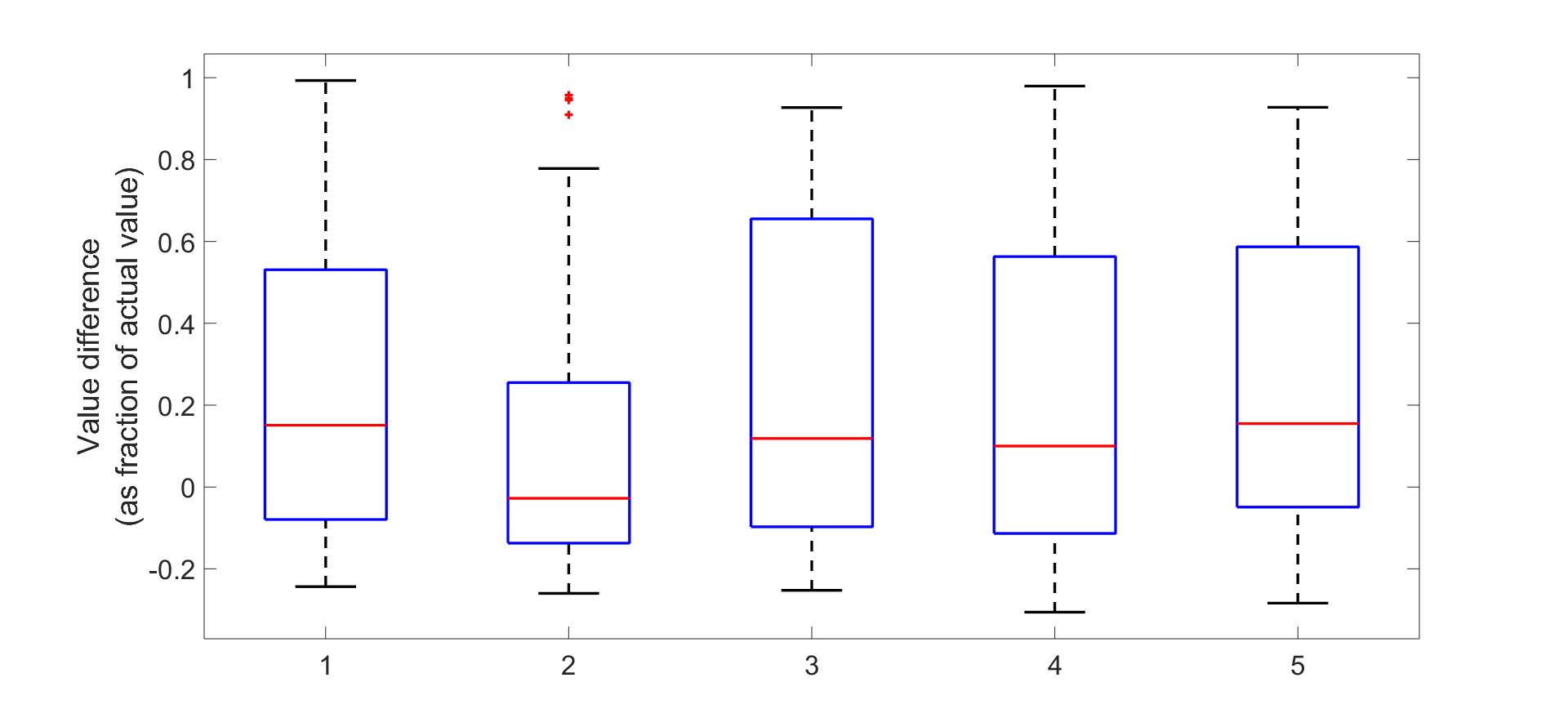
Utilizing a DQN provides no guarantees that the states seen during testing have been visited during training, which can lead to out-of-distribution states. Thus, we have to utilize a robust Student-t likelihood using the GP regression in GPFlow package [19]. The boxplots for the difference in values for 5 sample evaluation episodes are provided in Figure 3. Thus, we use these boxplots to show the value difference as a fraction of the actual value at that state and action. The boxplots show that the GP is able to recover a value close to the actual value (with zero being no difference and greater than $1$ meaning that the predicted value is not able to recover the actual value at all) for the majority of the episodes for continuous state domain problems.

References

- [1] D. M. Roijers, P. Vamplew, S. Whiteson, and R. Dazeley, “A survey of multi-objective sequential decision-making,” Journal of Artificial Intelligence Research, vol. 48, pp. 67–113, 2013.
- [2] G. Prokop, “Modeling human vehicle driving by model predictive online optimization,” Vehicle System Dynamics, vol. 35, no. 1, pp. 19–53, 2001.
- [3] K. Van Moffaert and A. Nowé, “Multi-objective reinforcement learning using sets of pareto dominating policies,” The Journal of Machine Learning Research, vol. 15, no. 1, pp. 3483–3512, 2014.
- [4] C.-L. Hwang and A. S. M. Masud, Multiple objective decision making—methods and applications: a state-of-the-art survey. Springer Science & Business Media, 2012, vol. 164.
- [5] S. Davies, “Multidimensional triangulation and interpolation for reinforcement learning,” in Advances in Neural Information Processing Systems, 1997, pp. 1005–1011.
- [6] C. Szepesvári, “Convergent reinforcement learning with value function interpolation,” Technical Report TR-2001-02, Mindmaker Ltd., Budapest 1121, Konkoly Th. M. u …, Tech. Rep., 2001.
- [7] P. Mannion, S. Devlin, K. Mason, J. Duggan, and E. Howley, “Policy invariance under reward transformations for multi-objective reinforcement learning,” Neurocomputing, vol. 263, pp. 60–73, 2017.
- [8] L. Barrett and S. Narayanan, “Learning all optimal policies with multiple criteria,” in Proceedings of the 25th international conference on Machine learning. ACM, 2008, pp. 41–47.
- [9] W. Wang and M. Sebag, “Multi-objective monte-carlo tree search,” 2012.
- [10] C. Williams and C. E. Rasmussen, “Gaussian processes for regression,” in Advances in neural information processing systems, 1996, pp. 514–520.
- [11] R. Bellman, “A Markovian decision process,” Journal of Mathematics and Mechanics, vol. 6, no. 5, pp. 679–684, 1957.
- [12] R. S. Sutton, D. A. McAllester, S. P. Singh, and Y. Mansour, “Policy gradient methods for reinforcement learning with function approximation,” in Advances in neural information processing systems, 2000, pp. 1057–1063.
- [13] C. E. Rasmussen, “Gaussian processes in machine learning,” in Summer School on Machine Learning. Springer, 2003, pp. 63–71.
- [14] R. S. Sutton and A. G. Barto, Reinforcement learning: An introduction. MIT press, 2018.
- [15] F. Pedregosa, G. Varoquaux, A. Gramfort, V. Michel, B. Thirion, O. Grisel, M. Blondel, P. Prettenhofer, R. Weiss, V. Dubourg, J. Vanderplas, A. Passos, D. Cournapeau, M. Brucher, M. Perrot, and E. Duchesnay, “Scikit-learn: Machine learning in Python,” Journal of Machine Learning Research, vol. 12, pp. 2825–2830, 2011.
- [16] S. Levine, Z. Popovic, and V. Koltun, “Nonlinear inverse reinforcement learning with gaussian processes,” in Advances in Neural Information Processing Systems, 2011, pp. 19–27.
- [17] G. Brockman, V. Cheung, L. Pettersson, J. Schneider, J. Schulman, J. Tang, and W. Zaremba, “Openai gym,” arXiv preprint arXiv:1606.01540, 2016.
- [18] V. Mnih, K. Kavukcuoglu, D. Silver, A. A. Rusu, J. Veness, M. G. Bellemare, A. Graves, M. Riedmiller, A. K. Fidjeland, G. Ostrovski et al., “Human-level control through deep reinforcement learning,” Nature, vol. 518, no. 7540, p. 529, 2015.
- [19] A. G. d. G. Matthews, M. van der Wilk, T. Nickson, K. Fujii, A. Boukouvalas, P. Le‘on-Villagr‘a, Z. Ghahramani, and J. Hensman, “GPflow: A Gaussian process library using TensorFlow,” Journal of Machine Learning Research, vol. 18, no. 40, pp. 1–6, apr 2017. [Online]. Available: http://jmlr.org/papers/v18/16-537.html
- [20] I. Das and J. E. Dennis, “A closer look at drawbacks of minimizing weighted sums of objectives for pareto set generation in multicriteria optimization problems,” Structural optimization, vol. 14, no. 1, pp. 63–69, 1997.