The Separation Distribution of Ultra-Wide Binaries
across Galactic Populations
Abstract
We present an extensive and pure sample of ultra-wide binary stars with separations of in the solar neighborhood. Using data from Gaia DR2, we define kinematic sub-populations via the systems’ tangential velocities, i.e., disk-like (), intermediate (), and halo-like () binaries, presuming that these velocity cuts represent a rough ordering in the binaries’ age and metallicity. Through stringent cuts on astrometric precision, we can obtain pure binary samples at such wide separations with thousands of binaries in each sample. For all three kinematic populations, the distribution of binary separations extends smoothly to 1 pc, displaying neither strong truncation nor bimodality. Fitting a smoothly-broken power law for the separation distribution, we find its slope at AU is the same for all sub-populations, with . However, the logarithmic slope of steepens at AU, to . We find some evidences that the degree of steepening increases with the binaries’ age, with a slope-change of only for disk-like stars, but for halo-like stars. This trend is contrary to what might be expected if steepening at wide separations were due to gravitational perturbations by molecular clouds or stars, which would preferentially disrupt disk binaries. If we were to interpret steepening at AU as a consequence of disruption by MACHOs, we would have to invoke a MACHO population inconsistent with other constraints. As a more plausible alternative, we propose a simple model to predict the separation distribution of wide binaries formed in dissolving star clusters. This model generically predicts as observed, with steepening at larger separations due to the finite size of binaries’ birth clusters.
Subject headings
binaries: general – binaries: visual – Galaxy: stellar content – stars: formation, statisticsI. Introduction
It has long been recognized that wide binaries provide a powerful tracer of the Galactic gravitational potential on small scales (Bahcall & Soneira 1981; Bahcall et al. 1985, e.g.) as well as useful constraints for studies of the star formation process (van Albada 1968; Chanamé 2007; Moeckel & Bate 2010; Kouwenhoven et al. 2010; Moeckel & Clarke 2011). The orbits of wide binaries are so fragile (with escape velocities km) that they can be easily unbound by external gravitational perturbations arising from molecular clouds, stars, or compact objects (Retterer & King 1982; Bahcall et al. 1985; Weinberg et al. 1987; Jiang, & Tremaine 2010; Allen & Monroy-Rodríguez 2014, e.g.), or by internal perturbations due to evolution of the component stars (Boersma 1961; Savedoff 1966; El-Badry & Rix 2018).
One of the most important applications of wide binaries is to constrain the mass of viable MAssive Compact Halo Objects (MACHOs), such as discrete black holes (BHs), which are a proposed dark matter candidate. Studies using wide binaries to constrain MACHOs have typically assumed a simple initial separation distribution (such as a smooth power law) and then interpreted deviations from it as arising from disruption of the widest binaries by MACHOs.
A number of previous studies have used halo wide binaries – which are expected to be less vulnerable to disruption by molecular clouds – to constrain the plausible parameters of MACHOs. Chanamé & Gould 2004 built a catalog of 1147 candidate wide binaries selected via common proper motion, from which they selected 801 binaries with disk-like orbits and 116 binaries with halo-like orbits. Fitting the two subsamples, they showed that the angular separation distributions could be well described by single power laws with logarithmic slopes of -1.670.07 for the disk binaries and -1.550.10 for the halo binaries, over the angular separation range . In a companion paper, Yoo et al. 2004 argued that the CG04 separation distribution constraints ruled out most of the previously plausible MACHO parameter space, since there was no strong evidence of a break in the separation distribution at the widest separations, and their simulations predicted a detectable break for MACHO masses .
When combined with constraints from microlensing surveys (which ruled out a dominant MACHO population with typical masses in the range of ; Alcock et al. 2001; Afonso et al. 2003) and theoretical lower limits on the long-term survivability of hydrogenous objects (which rule out MACHOs with ; de Rujula et al. 1992), the Y04 wide binary constraints ruled out almost all possible MACHO masses. Only a small window of MACHO masses, , was still considered viable. However, Quinn et al. 2009 later argued that the Y04 constraints depend critically on the validity of the two widest binaries in the CG04 sample. After removing one spurious candidate binary from the CG04 sample, they repeated the analysis of Y04 and found the wide binary separation distribution consistent with a MACHO mass of .
Precise proper motions and parallaxes from Gaia DR2 (Gaia Collaboration et al. 2016; Gaia Collaboration et al. 2018) have allowed the construction of larger and purer wide binary catalogs than were available previously. Distance measurements from Gaia parallaxes have also made it possible to measure the physical separation distribution; this is more easily interpretable than the angular separation distribution, whose physical scale depends on distance. El-Badry & Rix 2018 searched Gaia DR2 for high-confidence wide binaries within pc of the Sun. Their search yielded 55,000 high-confidence wide binaries, including 3,500 in which at least one component is a white dwarf. A similar search was carried out by Pittordis, & Sutherland 2019, who used the projected orbital velocities of Gaia wide binaries to constrain the gravitational force law in the low acceleration regime. Both of these studies limited their search to projected separations of AU (0.25 pc), primarily because the contamination rate from chance alignments would have become non-negligible at wider separations given their selection criteria. Because they searched for nearby binaries without any kinematic selection, the majority of the binaries in these samples have disk-like kinematics and roughly solar metallicity (El-Badry & Rix 2019, see).
Fitting the separation distribution with a broken power-law model, ER18 found that for MS/MS binaries, it was nearly consistent with a single power law of logarithmic slope but displayed evidence of a weak break at . They found the separation distributions for binaries containing a white dwarf to fall off more steeply at large separations and interpreted this steepening as evidence of non-adiabatic and/or asymmetric mass loss in the end stages of stellar evolution. The effects of disruption due to external perturbations are expected to become significant only at very wide separations ( AU; Weinberg et al. 1987), so ER18 did not attempt to constrain the effects of external perturbations using their sample.
In this paper, we (a) extend the ER18 analysis to wider separations and (b) compare the separation distributions of binaries between the Milky Way disk and halo. Constructing a large sample of halo binaries requires us to search to larger distances than ER18, but we show that it is still possible to obtain a high-purity binary sample at larger distances for halo stars, which have large proper motions and thus have fewer nearby neighbors in phase space. We kinematically select three pure subsamples with different average ages, using , the total tangential velocity with respect to the Sun, as a proxy of stellar age. By investigating the three binary populations, we try to answer three basic questions: (1) Is there a slope change in the separation distribution of wide binaries at AU, as found tentatively by ER18? (2) If so, does its strength vary between stellar populations? (3) Can it provide a meaningful constraints or clues on formation or destruction mechanisms of binaries in different populations?
Most previous works using wide binaries as dynamical tracers have implicitly assumed that the primordial separation distribution can be well-approximated as a simple power law at wide separations, and that it is the same for different populations. This is a serviceable assumption, and most previous works have found a power-law separation distribution to provide a good fit for wide binaries in the range of separations where external perturbations are expected to be subdominate (Lépine, & Bongiorno 2007; Andrews et al. 2017), but there is little a prior motivation for it. Now that the present-day separation distribution can be constrained in more detail, we reexamine this assumption.
The remainder of this paper is organized as follows. In Section 2, we describe how to build an initial the wide binary candidate catalog that is extensive but not pure. Sections 3 then presents three pure subsamples with different stellar populations selected from the candidate catalog, i.e., the disk-like, the kinematically intermediate, and the halo-like binaries. In Section 4, we illustrate the observed separation distributions for the three subsamples. In order to infer the intrinsic separation distributions, we describe the method in Section 5, including the selection function of the observed sample, a smoothly broken power law parameterization, and the likelihood for fitting the separation distribution. Section 6 lists the key results of the investigation. We discuss possible theoretical interpretations of our results in Section 7 and summarize in Section 8.
Throughout the paper, we adopt the Solar motion as km (Tian et al. 2015), and the circular speed of the local standard of rest (LSR) as km(Schönrich 2012). is used to denote the right ascension in the gnomonic projection coordinate system, for example, , and .
II. The Initial Wide Binary Candidate Catalog
We first construct a catalog of wide binary candidates that is large but not pure. In Section 3, we describe how pure subsamples can then be selected from the initial candidate catalog.
We select wide binary candidates with a procedure similar to that of ER18, whose catalog was restricted to pairs of stars within 200 pc of the Sun and projected separations pc. They selected stars whose positions, proper motions, and parallaxes were consistent with being gravitationally bound. For the present study, we extend the search volume from 200 pc to 4.0 kpc and the maximum projected separation from pc to pc. We briefly summarize the selection procedure below.
II.1. General criteria for the wide binary query
In the first step, we search for wide binary candidates that satisfy the following criteria:
- 1.
parallax , and parallax_over_error for the primary star. Possible companions are searched in a circle corresponding to a projected radius 1.0 pc around each primary, within an angular separation , where is the parallax of the primary star. The secondary companions are required to meet a lower threshold for parallax error, parallax_over_error (lower than the cut in ER18).
- 2.
Consistent distances for the primary and secondary. We require , where is the difference in distance between the two stars, is its uncertainty, and and represent the parallax of a primary or secondary and reported uncertainty. The term prevents us from missing the nearest and widest binaries, for which the orbital separation can be an non-negligible fraction of the distance.
- 3.
Small proper motion differences between the two stars, consistent with a bound Keplerian orbit. We require , where , which is the total scalar difference in proper motion between the two stars and is its uncertainty. represents the maximum proper motion difference permissible for a circular orbit of total mass . We also require the proper motions to be reasonably precise, with .
II.2. Quality cuts
We apply additional quality cuts on the astrometry and photometry of both components of candidate binaries:
- 1.
, to make sure that both members of a candidate binary pair have an acceptable astrometric solution (Lindegren et al. 2018). and are respectively referred to as astrometric_chi2_al and astrometric_n_good_obs_al in the Gaia archive.
- 2.
phot_bp_rp_excess_factor , to ensure that both stars have photometry that is relatively uncontaminated by nearby sources (Evans et al. 2018).
- 3.
phot_g_mean_flux_over_error50 for both member stars, phot_rp_mean_flux_over_error20 (10) for the primary (secondary) star, and phot_bp_mean_flux_over_error20 (10) for the primary (secondary) star, to remove pairs with low-SNR photometry.
These selection criteria yield an initial sample of 16,973,885 wide binary candidates.
II.3. Removing clusters, moving groups, and pairs in high density regions
Along with wide binaries, the criteria specified in Sections II.1 naturally select stars in bound clusters and moving groups. We remove these using a similar approach to that adopted by ER18.
For each candidate binary, we define nearby neighbor binaries as those that are within 1 degree on the sky, 3 mas in both proper motion coordinates, and 5 pc in . According to this definition, we count the number () of nearby neighbors in position-parallax-proper motion space, and remove candidate pairs that have nearby neighbors. 16,166,274 () pairs are removed in this step.
Because our binary candidate catalog is larger and contains fainter stars than the one constructed in ER18, the practical effect of this cut is different from the one applied in ER18. There, most of the candidate pairs removed were members of bound clusters. The cut here also removes clusters, but a large majority of the removed candidates are simply pairs in regions of high stellar density. As we discuss below, the contamination rate is high for such pairs anyway, so removing them is an acceptable concession.
This leaves 807,611 pairs as wide binary candidates.
II.4. Properties of the initial candidates
Figure 1 (top panel) shows a color-magnitude diagram (CMD) for all 807,611 (pairs) of wide binary candidates. The (primary) stars with are designated as “main sequence” stars (a few giants are not excluded), and the objects with are classified as likely white dwarfs (WDs). Here . The main sequence and red clump are visibly smeared out, primarily because the photometry is not corrected for extinction. Deviations from the expected CMD morphology are more pronounced for secondaries, (top right panel in Figure 1) because the cuts on astrometric and photometric precision (Section II.2) are looser for secondaries. A large cloud of objects is visible between the white dwarfs and main sequence for secondaries. These are primarily sources with large parallax errors; they are removed from the sample once more stringent quality cuts are applied (See lower panels of Figure 1). A secondary sequence is apparent above the main sequence for both primaries and secondaries, indicating that the catalog contains hierarchical triples with components that are spatially unresolved close binaries.
Figure 2 (top panel) presents the sky distribution of all binary candidates in the vs. plane, where and represent galactic latitude and longitude. Clear imprints of the Gaia scanning law are apparent, as there are more sources with well-constrained astrometry in regions of the sky that were visited more often. An higher density of candidates is also apparent near the galactic plane; this was even more pronounced prior to the removal of sources with many phase-space neighbors. A few blank patches at are very dense regions where our queries timed out and no candidates could be identified.


Figure 3 illustrates the distributions of distance (, first column), magnitude difference (, second column), apparent magnitude (, third column), and angular separation (, fourth column) for all wide binary candidates (black). The distribution of physical separation is displayed separately in Figure 4. For the initial candidate sample, the distributions are dominated by contaminants (chance-alignments) at large separations ( arcmin and pc). This can be seen in the distributions of and , where the large-separation peak is due entirely to chance alignments. We discuss chance-alignment further below.
II.5. Contamination rates of the initial sample
We use three methods to quantify the contamination rates of the candidate binaries as a function of separation: (1) A “shifted Gaia DR2 catalog”, where the coordinates (, ) for each object in this catalog have been constructed by shifting 1° from its original location (, ), i.e., (, ) = ( + , + ), with °. We then repeat the binary candidate identification procedure, now identifying pairs that pass the binary cuts when the coordinates of the “primary” are shifted relative to candidate secondaries. This procedure removes genuine binaries, but preserves chance alignment statistics; see Lépine, & Bongiorno 2007 for further discussion of this method of estimating the chance alignment rate. (2) The mock Gaia DR2 catalog produced by Rybizki et al. 2018, which is based on the Besançon stellar population synthesis model (Robin et al. 2003) and is populated with the Galactic distribution function using Galaxia (Sharma et al. 2011), assuming a similar selection function and uncertainty model to Gaia DR2. (3) Comparison of radial velocities (RVs) for the subset of bright wide binaries where both stars have RVs included in Gaia DR2.
The red dotted curves in Figure 3 present the distributions of the random alignment pairs chosen from the shifted Gaia DR2 catalog in the whole sky. We matched the original Gaia DR2 with the shifted catalog, and regard the matched pairs as chance alignments if they pass the selection criteria for binaries. This approach is not appropriate for the widest and most nearby binaries, which can have projected separations of or larger, and so continue to appear as binaries even when the coordinates of one component are artificially shifted by in each direction. Therefore, we remove the chance alignments with d 60 pc and 0.5° from the shifted catalog. The red dotted curves suggest that the distributions for the initial candidates are indeed almost fully dominated by contaminants at large angular and projected separations, as displayed in the last two sub-panels of Figure 3. On the other had, chance alignments are subdominant at (Figure 3). The distribution of chance alignments can be well described as , since the area within which chance alignments can be found scales as .
We selected in a random region of from the mock Gaia DR2 catalog (Rybizki et al. 2018). The mock catalog does not contain any true binaries, so any pairs that pass our selection criteria in the mock catalog must be chance alignments. We only query a fraction of the sky in the mock catalog because querying it is computationally expensive and many of the queries time out. In estimating the true contamination rate, we scale up the rate predicted by the mock catalog at all separations, assuming the contamination rate approaches 100% at 1 pc separations.
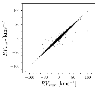
In defining candidate wide binaries in this study, we used the two dimensional velocities (i.e., 2-D tangential velocities from proper motions), positions and distances. The incomplete kinematic information induces substantial contamination, particularly at large separations. Gaia DR2 provides about 7.2 million stars with measured RVs. Among them, 8220 wide binary candidates have reliable (uncertainty km) RVs for both binary components. These RVs provide the third dimension of velocity and can be effectively used to check whether candidate pairs are true binaries or chance alignments. Significant RV differences () between member stars imply that star pairs are probably chance alignments. We regard those pairs with and km as likely contaminants. Figure 5 displays the 1-to-1 scatter distribution (the top panel) of the two component RVs, and the distribution (the bottom panel) as a function of projected separation. Only 20 pairs meet the criteria of chance alignments, i.e., and km. Most binaries with substantially large have larger-than-average RV uncertainties. This implies that the contamination rate of the candidate binary catalog is of order 0.24%, with most contaminants at , for binaries that are bright enough for both stars to have measured RVs (). However, we stress that the true contamination rate for the whole catalog of binary candidates is much higher, as can be seen in Figure 3. The RVs provide an estimate of the chance-alignment rate for binaries where both components are bright.
Table 1 summarizes the contamination rates in the different projected separation bins, estimated with the above three methods.

. Separations Contamination Rates log(s/AU) Mock11footnotemark: 1 Gaia RVs22footnotemark: 2 Shifted Gaia DR233footnotemark: 3 All Disk Intermediate Halo All Disk Intermediate Halo All Disk Intermediate Halo (0.00, 3.40] 0% 0% 0% 0% 0% 0% 0% 0% 0.3% 0% 0% 0% (3.40, 4.12] 2% 0% 0% 0% 0.1% 0% 0% 0% 2% 0% 0% 0% (4.12, 4.39] 10% 0% 0% 0% 0.1% 0% 0% 0% 10% 0% 0% 0% (4.39, 4.65] 30% 0% 0% 0% 0.2% 0% 0% 0% 30% 0% 0% 0% (4.65, 4.91] 80% 0% 0% 0% 0.4% 0% 0% 0% 80% 1% 0.1% 1% (4.91, 5.20] 90% 0% 0% 0% 1.5% 0% 0% 0% 90% 0% 1% 5% (5.20, 5.31] 95% 0% 0% 0% 11% 0% 0% 0% 95% 0% 10% 15%
- a
Using the mock catalog from Rybizki et al. 2018 to estimate the contamination rate, assuming the contamination for the initial candidates reaches 100% at the widest separations.
- b
Using the reliable ( km) Gaia radial velocities (RVs) to estimate the contamination rate of the the brightest wide binaries, where both components have . Pairs with and km are regarded as chance alignments.
- c
Using the shifted Gaia DR2 to estimate the contamination rate. Each object is shifted by 1° in each coordinate i.e., (, ) = ( + 1.0°, + 1.0°), where (, ) and (, ) are the shifted and original coordinates, respectively.
III. Three Pure Binary Samples with Different Kinematic Ages
As low contamination is crucial for our subsequent analysis of the separation distributions, we proceed to define subsamples that we can assume to be nearly pure. Specifically, we kinematically select three pure subsamples, consisting of young disk-like, intermediate, and old halo-like binaries, with different average ages. Since the phase-space density of contaminants varies between the samples (with more contaminants in the low-velocity samples), we use different quality cuts for the three samples.
Using the Gaia DR2 proper motion and parallax, we calculate the total tangential velocity with respect to the Sun for each candidate binary:
| (1) |
Here and are the parallax and total proper motion of a binary, respectively.
Using as a proxy of age, we select three pure subsamples with different average ages. We determine what cuts are needed to obtain a pure subsample in each population using the shifted catalog the estimated the chance alignment rate given any sub-selection.
The space density of halo stars in the solar neighborhood is much lower than that of disk stars, so it is necessary to search to larger distances to obtain a large sample of halo binaries. Fortunately, the contamination rate at fixed distance is also much lower for halo stars, because they have fewer phase-space neighbors. We thus use different distance limits for the three populations and self-consistently estimate the contamination rate for each population given these limits. We choose disk-like binaries with
- 1.
d 120 pc,
- 2.
km.
To select the intermediate-age binary subsample, we use the conditions:
- 1.
d 300 pc,
- 2.
km.
We choose old halo-like binaries with the following criteria,
- 1.
d 700 pc,
- 2.
km.
To get pure binary samples, we further impose the following cuts on all of the above three selections:
- 1.
and . This more stringent cut on proper motion uncertainty reduces the contamination from chance alignments with larger uncertainty.
- 2.
The number of nearby neighbors , to strictly remove contaminants at wide separation from moving groups or star clusters.
- 3.
We exclude binaries containing a WD from all three subsamples to remove the effect from internal orbital evolution.
The above criteria can effectively suppress the three kinds of contamination rates close to zero for the three subsamples at each (except the largest) separation bin (see Table 1). Finally, we get 4361 disk-like, 10,090 intermediate and 4351 halo-like genuine wide binaries. Figure 4 compares the separation distributions of binaries and chance-alignments in the three subsamples. With these more aggressive cuts on distance and astrometric SNR, chance alignments are subdominant out to separations of 1,pc. The separation distributions of all three samples fall off monotonically at large separations.
Figure 1 displays the color-magnitude diagrams (CMD) for the disk-like (blue), intermediate (green) and halo-like (magenta) wide binaries. The unresolved close binary sequences (Widmark et al. 2018, ER18;) are visible but already sparse above the main sequence in the three subsamples. Following ER18, we use the region at of the CMD (Figure 1) to estimate the unresolved binary fraction of the disk and halo samples. In this region, the line divides the binary and single-star main sequences. We find that about 4.0% (4.3%), 10.9% (7.4%) and 6.6% (4.8%) of the primary (secondary) disk-like, intermediate and halo-like binaries probably have a bright unresolved companion.
Figure 2 presents the final disk-like (the 4361 blue dots), intermediate (the 10,090 green dots) and halo-like (the 4351 magenta dots) binaries distribution in the vs. plane. Figure 3 illustrates the distributions of distance (, first column), magnitude difference (, second column), magnitude (, third column), and angular separation (, fourth column), respectively, for the three subsamples. For demonstrating the contamination rate, the distributions of projected separations () for the three subsets are specifically displayed in Figure 4. In this figure, the blue, green and magenta dotted curves show the distributions of the chance alignments selected from the shifted catalog with the disk-like, intermediate and halo-like criteria, respectively.
We use the mock Gaia DR2 catalog (Rybizki et al. 2018) to illustrate the effect of for distinguishing the three subsamples. The mock catalog contains the full 6-D phase information for each star, so the disk-like, intermediate and halo-like stars are easily separated. We randomly select 150,000 stars in the whole sky from this mock catalog and use the criteria of to separate the mock stars into disk-like, intermediate and halo-like populations. Figure 6 shows the Toomre diagram for disk-like stars (blue points), intermediate (green points), and halo-like stars (magenta points). As one can see, the disk-like, intermediate and halo-like stars are clearly divided. This indicates that the criteria of work well for the selection of the three kinematic subsamples.

IV. Observed Separation Distributions
We display distributions of the angular () and the projected physical separations ( AU) for the disk-like, intermediate, and halo-like binaries in Figure 3 (the last sub-panels) and Figure 4. At arcsec, there are no binaries in our sample, which is due to the Gaia angular resolution limit. At or ( for the halo-like binaries), the samples are significantly incomplete. ER18 investigated this incompleteness effect and concluded that the incompleteness is due to blending of the two stars, which is more severe for binaries with magnitude difference between the two components. According to Figure A1 of ER18, the separation distribution is 84% complete for at arcsec and is complete for all at arcsec, relative to the completeness at arbitrarily large angular separations.
Consistent with ER18, we find that the main sequence binaries do not obey Opik’s law (i.e., a flat distribution of log-separation) at any AU. It is worthwhile to mention that there is an obvious drop at AU in the raw separation distributions of the three subsamples, as shown in Figure 4.
We note that, when insufficiently stringent astrometric quality cuts are applied, the separation distribution of all binary candidates in Figure 4 appears bimodal (black histogram). However, the peak at large separations is due entirely to chance alignments, not real binaries. For this reason, it shifts toward wider separations and eventually disappears as more stringent quality cuts are applied. Some previous works (Dhital et al. 2010; Oelkers et al. 2017) have found the separation distribution of wide binaries to be bimodal and have proposed that the wider-separation population contains binaries formed by different formation mechanism. Our analysis suggests that this apparent bimodality is simply due to chance alignments, as also suggested by Andrews et al. 2017.
V. Inferring Intrinsic Separation Distribution
As discussed in Section IV, the separation distribution at arcsec is heavily incomplete. Before modeling the intrinsic-separation distribution, one must account for the selection effect to compensate for the incompleteness at small separation. In this section, we directly adopt an empirical fitting function from ER18 as the selection function, and we use a smoothly broken power law with four free parameters to model the intrinsic-separation distribution.
V.1. Selection Function
The selection function depends on the angular separation and the magnitude contrast between the two member stars. For this study, we empirically characterize the probability of detecting a companion at an angular separation with a fitting selection function found by ER18,
| (2) |
Here is the magnitude contrast in -band between the two member stars, characterizes the angular separation below which the sensitivity drops to 0, and determines how rapidly the sensitivity falls off at . Following ER18, we adopt for all , arcsec at mag, and at mag. We stress that does not represent the absolute selection function, but rather the fraction of binaries detected at angular separation relative the the number that would be detected at arbitrarily large separation. See El-Badry et al. 2019, their Appendix D, for details.
V.2. Function form of the separation distribution
We model the separation distribution as a smoothly broken power law:
| (3) |
where is a normalization parameter. The break separation marks the transition between the two single power laws with index and , respectively. The parameter quantifies how abruptly or smoothly the two power laws are joined. The model has four fit parameters . We suppose that is independent of both the distance and the absolute magnitude of the two member stars, although the separation distribution is expected to vary somewhat with the mass (and thus, absolute magnitude) of the two stars (Duchêne & Kraus 2013; Moe, & Di Stefano 2017; Moe & Kratter 2018, e.g.,). This supposition is validated with two special datasets selected from the pure samples: one with mag, which contains 1633 disk-like, 3481 intermediate, and 986 halo-like binaries; the other one with mag, which includes 2287 disk-like, 6684 intermediate, and 3542 halo-like binaries. The analysis on these datasets indicates that the large or stellar mass just slightly affects the shape of the observed separation distribution at small separations, and this selection effect can be well overcome with the selection function when the intrinsic separation distribution is derived in the following section.
V.3. Likelihood for Fitting the Separation Distribution
Given a sample of binaries with projected separations , the likelihood function is
| (4) |
where is a set of free model parameters to be fitted and is the probability of detecting the -th binary given model parameters . For the -th binary, can be specified
| (5) |
where is the probability that a binary with distance , magnitude difference , and physical separation is found in the catalog, given an intrinsic-separation distribution (specified by Equation (3)) with parameters . The selection function, , is given by Equation (2). Here and are the minimum and maximum separations of the observed distribution in the disk and halo binary samples, and is normalized such that . Equation (5) does not account for the observational uncertainties in or . These are small because all the binaries in our clean samples have parallax errors smaller than 5%.
The denominator in Equation (5) reflects the fraction of predicted binaries that could have been detected at a distance and magnitude difference ; it accounts for the fact that at large distances and large , only binaries with large can be detected. We set AU (i.e., pc), omitting the widest separation bin due to a high contamination rate beyond AU. The choice of has no effect on our results because the integrand in Equation (5) goes to 0 at small separations. We set AU.
If either member star of a binary is too faint, the binary probably can not be detected. Therefore, whether a binary can be observed or not also depends on the apparent magnitude of both stars. However, this has no effect on the inferred separation distribution as long as the undetected binaries have the same intrinsic separation distribution.
VI. Results
We use emcee (Foreman-Mackey et al. 2013) to sample the posterior distribution of the broken-power-law model of binary separations (Eq.3), for the three subsamples of disk-like, intermediate and halo-like binaries. We use flat priors for , , and and use an exponential prior on , taking a prior of ) for . The top panel of Figure 7 displays the contours and marginalized probabilities of the model parameters posteriors , while the bottom panel illustrates the inferred intrinsic separation distributions for the three subsamples. The median values of are
- •
for the disk-like binaries,
- •
for the intermediate binaries
- •
for the halo-like binaries.
These results, which are illustrated in Figures 7, can be summarized as follows:
- 1.
At , the three subsamples have the same separation distributions, i.e., a power law with an index of shown as the black dashed lines in the bottom panels of Figure 7.
- 2.
At , the separation distributions become significantly steeper for all three subsamples, excluding single power-law models over the entire separation range (see the bottom panel of Figure 7). This profile steepening () increases from 0.560.50 for the disk-like binaries, through 0.60 for the intermediate binaries, to 1.780.70 for the halo-like binaries. There is thus a strong hint of a steeper fall-off at ultra-wide separations ( AU) for the halo-like sample than the disk sample, although the marginalized constraints on are quite broad due to degeneracies with other parameters.
- 3.
The for the disk-like sample is significant, but small enough to explain why ER18 found comparably good fits for MS/MS binaries with a single power law with a slope -1.6 over . The for the halo-like sample, however, indicates a quite substantive change in the separation distribution slope at AU (i.e., 0.1 pc).
- 4.
The smoothing parameter differs among the subsamples: the halo-like subsample has the strongest break (highest ), yet the smoothest power-law transition, i.e. the highest parameter .
- 5.
The posterior distributions of the free parameters (except ) gradually present a double-peak feature from the disk-like to the halo subsamples. It indicates that the intrinsic separation distributions favor two breaks for all the three subsamples, in particular for the old population. One break takes place at AU, the corresponding smoothing parameter is . The other break is at AU and its .
- 6.

VII. Interpreting Separation Distributions
At smaller separations, the observed separation distribution of binaries presumably reflects a combination of birth separations and subsequent evolution (e.g. El-Badry et al. 2019; Liu 2019; Moe, & Di Stefano 2017, and references therein). For the very wide binaries (beyond a few AU) of primary interest here, the formation process leading to the ”initial” separation distribution at the time of birth cluster dispersal, and the subsequent evolutionary processes, are not firmly established. Wide binaries presumably did not form within a common disk, but resulted from turbulent fragmentation (at closer separations) and stochastic pairing during cluster dissolution (at wider separations). After formation, wide binaries could retain their original orbital parameters, except (1) that they may be affected or become disrupted by gravitational encounters with molecular clouds or other massive objects (Chanamé & Gould 2004, e.g.); (2) that either one or both binary members evolve off main sequence, inducing rapid mass loss (e.g. ER18); or (3) that dynamical evolution leads to widening within unstable triples (Reipurth, & Mikkola 2012, e.g.).
This present work was originally initiated with the goal of detecting or constraining signs of binary disruption by massive objects. In such an analysis one must presume to have confident prior knowledge about the initial separation distribution to pc, e.g. that it was a perfect single power-law at large . We first pursue this approach of modeling, asking what population of massive scattering objects could lead to the breaks seen. This, however, turns out to have physically implausible implications, at variance with other constraints. In light of this we then ask what separation distribution we may have expected at birth, and find it to be consistent with the observations.
VII.1. An initial single power law, broken
by a population of scatters?
We start out by noting that the outer slope of the disk-like binary is if anything flatter than that of the halo-like populations, showing a steepening by only : this argues against, or at least provides not evidence for, molecular clouds being a dominant mechanism is setting the outer slope of wide disk-like binaries by means of tidal disruption that would induce a cut-off.
We now use the approach of previous studies, assuming that the separation distribution for wide binaries follows a single (initial) power law. By implication, any break in such power law is then attributed to external perturbations, e.g., binary disruption as a consequence of encountering MACHOs. Disk-like binaries are more likely to encounter molecular clouds - acting as perturbers - during much of their orbits, and any such encounters will be at lower velocities. It has therefore been inferred (Chanamé & Gould 2004, e.g.) that such samples should not be used to probe the properties of MACHOs, as their perturbative effect would be subdominant. However, halo binaries spend only a small fraction of their lifetime in the disk and cross it at high speed, so MACHOs (if they exist) could be the dominant perturbers, with the observed separation distribution providing constraints on their density and mass.
Such external perturbations can be usefully divided into two regimes: a diffusive regime in which perturbations are described by a multitude of individually weak gravitational encounters, and a catastrophic regime in which perturbations are dominated by a single closest encounter. As described in Section VI, we detect steepening at pc in the separation distribution, which is particularly distinct for the halo-like subsample.
For those two disruption regimes (Binney & Tremaine 2008, Eq. 8.65a and b), the timescales to disrupt a solar mass binary at a separation of pc can be expressed as:
| (6) |
and
| (7) |
Here, is the relative velocity of a MACHO perturber passing by one of binary components, is the individual mass of the perturbers, and is their mean mass density near the Sun. The local halo mass density is denoted by , and we adopted M⊙pc-3. In the catastrophic regime, the disruption timescale at a given separation is independent of the mass and velocity of the perturber, set merely by . If the perturber mass
| (8) |
would be shorter than the typical time, i.e., 10 Gyr. The condition to see a distinct break due to disruption in the diffusive regime is . Therefore, M⊙, marks the transition between the two regimes. Previous authors expected to see a signature of binary separation function at pc in the several studies (Quinn et al. 2009, CG04; Y04;), but failed to detect the break signature due to the paucity of observational wide binaries at large separations.
However, the implied lower limits on the MACHO density or MACHO mass implied by the above analysis (critically hinging on the assumption of an initial single power law for the binary separations) would be in direct conflict with the the stringent upper limits from the survival of compact ultra-faint dwarf galaxies and the star cluster in Eridanus II. With these latter systems, Brandt 2016 closed the window of allowed MACHO mass in M⊙, and thereby ruled out the entire window of MACHO mass in M⊙ by combining his results with the existing constraints (Tisserand et al. 2007; Wyrzykowski et al. 2008; Quinn et al. 2009; Green 2016, Y04;). We also note that the steepening in the observed separation distributions is relatively gradual, and is not manifest as a sharp truncation or break. The arguably most obvious way to resolve this tension is to acknowledge that the assumption of an initial single power law was too restrictive, and not realized in nature.
VII.2. A simple model for the primordial
wide-binary separation distribution
We now lay out a very simple model for the separation distribution of wide binaries (wider than a few 1000 AU) that might be expected as a consequence of their formation. Given their dynamical fragility, we presume that most could have formed only as the cluster (or association) was dispersing. A pair of stars in a dispersing star cluster at separation will be and presumably remain bound provided that , where is the total mass of the pair and is their total relative velocity. For a Gaussian velocity distribution (the velocity dispersion of the birth cluster), and for “wide binaries” (), this will occur with probability,
| (9) |
for separations smaller than the cluster’s tidal radius, . Here we have taken into account the fact that while phase space available to yield scales , the in this expression is canceled for a typical cluster profile , within , with no pairs larger than this radius.
Thus for an ensemble of dissolving clusters with characteristic tidal radii , the separation distribution of subsequently bound wide pairs for will always be the same (i.e., , ); the sum of such distribution will have the same power law. However, as these clusters will not all have the same , the individual-cluster distributions will have breaks at . Hence, for , the joint distribution will be characterized by a true power law, while for it will fall off more rapidly in a manner that presumably could be approximated as a power law, depending on the statistics of .
This simple model has two attractive features in this context. First, it provides an explanation of why wide binaries in the range AU to AU have a separation distribution of across all populations. And it implies that the birth cluster size has an imprint on the (maximal) binary separation distribution even long after the cluster has been dispersed. If stars born in earlier epochs of the Milky Way’s evolution (viz. the halo-like population) formed in clusters that were more compact (smaller ), or with a narrower distribution of among the clusters, then their separation distribution should experience a more distinct departure from the power law. On the other hand, halo binaries are subject to fewer gravitational perturbations due to their higher velocities. These two effects work in opposite directions and it is not immediately clear which will dominate. The fact that the observed separation distributions across the three samples are quite similar even at wide separations suggests that they partially cancel. If the clusters that gave birth at a later epoch to the disk-like binaries had a wider distribution of , e.g. because a larger fraction of them were born in barely-bound associations, then we would expect a less distinct break in the separation power-law. In this model, the present-day separation distribution is still mostly a reflection of the initial distribution. Of course, some tidal disruption may have played a role as approaches one parsec. Note also, that this model can only infer - not predict - the break radius, , which is larger for the halo-like binaries than for the disk-like ones.
VIII. Conclusion
We have compiled an extensive yet pure catalog of candidate wide binaries ( pc) selected from Gaia DR2 in the solar neighborhood with distances kpc, following a procedure similar to that of ER18. This initial candidate catalog consists of 807,611 possible binaries. Its contamination rates are lower than 10% at AU; however, the contamination rates quickly increase beyond 20,000 AU, until up to 100% at the largest separation bin, i.e., pc. To address this, we subsequently applied additional selection criteria, tailored towards three kinematically-selected, presumably pure subsamples: disk-like, intermediate, and halo-like binaries. The raw catalog is described in Table 2, which will be released on-line and available via the PaperData Service of China-VO.
This raw catalog of candidate wide binaries can provide a starting point for several scientific applications beyond the scope of this paper. For instance, one could select a subsample of wide binaries containing a WD member from the raw catalog to determine stellar ages. The age of a WD can be easily constrained from its cooling age and mass given an initial-final mass relation and an initial mass-age relation, while the age of its companion MS star could not be measured precisely. The two members in a binary usually can be regards to be co-eval, so the MS star’s age can be simply obtained from its companion WD star (Fouesneau et al. 2019).
To reach low contamination to separations of pc, we defined three subsamples of MS-MS binaries from the raw catalog via the systems’ projected velocities with respect to the Sun, : 4361 disk-like binaries with km/s, 10,090 kinematically intermediate binaries with km/s km/s, and 4351 binaries with halo-like kinematics ( km/s). We presume that these velocity cuts represent a rough ordering in the binaries’ age. Using three catalogs, i.e., the mock Gaia DR2 catalog (Rybizki et al. 2018), a shifted Gaia DR2 catalog, and around 7.2 million Gaia DR2 stars with RVs, we quantify the contamination rates of the three subsamples after we have applied additional cuts in the different separation bins, and find that the contamination rates in the three subsamples are negligible in the range of separation pc.
We then proceeded to model the separation distributions of these subsamples as a smoothly broken power law, with four free parameters . Fitting these model for the three subsamples for AU and accounting for the selection function, several important findings have been discovered: (1) we confirm that the slope for separations from AU to AU is , as found in previous studies; this slope is essentially the same for all three subsamples. (2) we show for the first time at high significance how the slope steepens beyond AU; and we find first tentative evidence that this slope-steepening differs among these sub-populations: by only for stars of disk-like kinematics, but by for stars with halo-like kinematics. The actual values of would be even larger than these estimates, if we had unrecognized contamination at the largest separations. (3) we also find some, albeit tentative, evidence that increases from AU for the disk-like subsample to AU for the halo-like subsample.
We have offered interpretations for these observational findings in the two limiting cases: we start by presuming that the birth separation was a single power-law to pc, altered only by binary disruption effected by some possible MACHO populations. The break in pc in the separation distribution of the halo-like subsample, would imply M⊙ at a very high mean MACHO density. However, this window of MACHO candidates has been closed by other studies, e.g., Brandt 2016, and we must conclude that – in light of a complex, but not truncated, separation distributions – MACHO limits or detections would be hard to derive, as no clearly defined null-hypothesis for the undisturbed separation distribution exists.
We therefore build a conceptually different simple model asking what we should expect for the initial (birth) separation distribution. We find that a simple model, where binaries form by stars remaining stochastically bound as the cluster disperses, works remarkably well in two respects: in generically predicts a distribution power law of , as observed in all populations. And it implies that the separation distribution will steepen beyond separations in excess of the initial cluster size; therefore, (expected) structural differences between the birth clusters or associations of the different populations may now be reflected in the separation distribution of ultra-wide binaries.
References
- Afonso et al. (2003) Afonso, C., Albert, J. N., Andersen, J., et al. 2003, A&A, 400, 951
- Alcock et al. (2001) Alcock, C., Allsman, R. A., Alves, D. R., et al. 2001, ApJ, 550, L169
- Allen & Monroy-Rodríguez (2014) Allen, C., & Monroy-Rodríguez, M. A. 2014, ApJ, 790, 158
- Andrews et al. (2017) Andrews, J. J., Chanamé, J., & Agüeros, M. A. 2017, MNRAS, 472, 675
- Badenes et al. (2018) Badenes, C., Mazzola, C., Thompson, T. A., et al. 2018, ApJ, 854, 147
- Bahcall & Soneira (1981) Bahcall, J. N., & Soneira, R. M. 1981, ApJ, 246, 122
- Bahcall et al. (1985) Bahcall, J. N., Hut, P., & Tremaine, S. 1985, ApJ, 290, 15
- Batista et al. (2011) Batista, V., Gould, A., Dieters, S., et al. 2011, A&A, 529, A102
- Binney & Tremaine (2008) Binney, J., & Tremaine, S. 2008, Galactic Dynamics: Second Edition
- Brandt (2016) Brandt, T. D. 2016, ApJ, 824, L31
- Boersma (1961) Boersma, J. 1961, Bull. Astron. Inst. Netherlands, 15, 291
- Chanamé & Gould (2004) Chanamé, J., & Gould, A. 2004, ApJ, 601, 289
- Chanamé (2007) Chanamé, J. 2007, Binary Stars as Critical Tools & Tests in Contemporary Astrophysics, 316
- Dhital et al. (2010) Dhital, S., West, A. A., Stassun, K. G., et al. 2010, AJ, 139, 2566
- Duchêne & Kraus (2013) Duchêne, G., & Kraus, A. 2013, ARA&A, 51, 269
- de Rujula et al. (1992) de Rujula, A., Jetzer, P., & Masso, E. 1992, A&A, 254, 99
- El-Badry & Rix (2018) El-Badry, K., & Rix, H.-W. 2018, MNRAS, 480, 4884
- El-Badry & Rix (2019) El-Badry, K., & Rix, H.-W. 2019, MNRAS, 482, L139
- El-Badry et al. (2019) El-Badry, K., Rix, H.-W., Tian, H., et al. 2019, MNRAS, 489, 5822
- Evans et al. (2018) Evans, D. W., Riello, M., De Angeli, F., et al. 2018, A&A, 616, A4
- Fouesneau et al. (2019) Fouesneau, M., Rix, H.-W., von Hippel, T., et al. 2019, ApJ, 870, 9
- Foreman-Mackey (2016) Foreman-Mackey, D. 2016, The Journal of Open Source Software, 1, 24
- Foreman-Mackey et al. (2013) Foreman-Mackey, D., Hogg, D. W., Lang, D., et al. 2013, PASP, 125, 306
- Gaia Collaboration et al. (2016) Gaia Collaboration, Brown, A. G. A., Vallenari, A., Makarov, V. V., et al. 2016, A&A, 595, A2
- Gaia Collaboration et al. (2018) Gaia Collaboration: Brown, A. G. A., Vallenari, A., Makarov, V. V., et al. 2018, A&A, 616, A1
- Green (2016) Green, A. M. 2016, Phys. Rev. D, 94, 063530
- Kouwenhoven et al. (2010) Kouwenhoven, M. B. N., Goodwin, S. P., Parker, R. J., et al. 2010, MNRAS, 404, 1835
- Lépine, & Bongiorno (2007) Lépine, S., & Bongiorno, B. 2007, AJ, 133, 889
- Liu (2019) Liu, C. 2019, arXiv e-prints, arXiv:1907.02250
- Lindegren et al. (2018) Lindegren, L., Hernández, J., Bombrun, A., et al. 2018, A&A, 616, A2
- Moe, & Di Stefano (2017) Moe, M., & Di Stefano, R. 2017, ApJS, 230, 15
- Moe & Kratter (2018) Moe, M., & Kratter, K. M. 2018, ApJ, 854, 44
- Moeckel & Bate (2010) Moeckel, N., & Bate, M. R. 2010, MNRAS, 404, 721
- Moeckel & Clarke (2011) Moeckel, N., & Clarke, C. J. 2011, MNRAS, 415, 1179
- Oelkers et al. (2017) Oelkers, R. J., Stassun, K. G., & Dhital, S. 2017, AJ, 153, 259
- Pittordis, & Sutherland (2019) Pittordis, C., & Sutherland, W. 2019, MNRAS, 1859
- Quinn et al. (2009) Quinn, D. P., Wilkinson, M. I., Irwin, M. J., et al. 2009, MNRAS, 396, L11
- Raghavan et al. (2010) Raghavan, D., McAlister, H. A., Henry, T. J., et al. 2010, ApJS, 190, 1
- Reipurth, & Mikkola (2012) Reipurth, B., & Mikkola, S. 2012, Nature, 492, 221
- Retterer & King (1982) Retterer, J. M., & King, I. R. 1982, ApJ, 254, 214
- Robin et al. (2003) Robin, A. C., Reylé, C., Derrière, S., et al. 2003, A&A, 409, 523
- Rybizki et al. (2018) Rybizki, J., Demleitner, M., Fouesneau, M., et al. 2018, PASP, 130, 74101
- Jiang, & Tremaine (2010) Jiang, Y.-F., & Tremaine, S. 2010, MNRAS, 401, 977
- Savedoff (1966) Savedoff, M. P. 1966, AJ, 71, 396
- Sharma et al. (2011) Sharma, S., Bland-Hawthorn, J., Johnston, K. V., et al. 2011, ApJ, 730, 3
- Schönrich (2012) Schönrich, R. 2012 MNRAS, 427, 274
- Tian et al. (2015) Tian, H.-J., Liu, C., Carlin, J. L., et al. 2015, ApJ, 809, 145
- Tisserand et al. (2007) Tisserand, P., Le Guillou, L., Afonso, C., et al. 2007, A&A, 469, 387
- van Albada (1968) van Albada, T. S. 1968, Bull. Astron. Inst. Netherlands, 20, 57
- Wyrzykowski et al. (2008) Wyrzykowski, L., Kozlowski, S., Belokurov, V., et al. 2008, Manchester Microlensing Conference, 11
- Wasserman, & Weinberg (1987) Wasserman, I., & Weinberg, M. D. 1987, ApJ, 312, 390
- Weinberg et al. (1987) Weinberg, M. D., Shapiro, S. L., & Wasserman, I. 1987, ApJ, 312, 367
- Widmark et al. (2018) Widmark, A., Leistedt, B., & Hogg, D. W. 2018, ApJ, 857, 114
- Yoo et al. (2004) Yoo, J., Chanamé, J., & Gould, A. 2004, ApJ, 601, 311
- Zapatero Osorio, & Martín (2004) Zapatero Osorio, M. R., & Martín, E. L. 2004, A&A, 419, 167
| Column | units | Description |
|---|---|---|
| source_id | Gaia source id (int64); star 1 | |
| source_id2 | Gaia source id (int64); star 2 | |
| astrometric_chi2_al | astrometric goodness-of-fit () in the along-scan direction; star 1 | |
| astrometric_chi2_al_2 | astrometric goodness-of-fit () in the along-scan direction; star 2 | |
| astrometric_n_good_obs_al | number of good CCD transits; star 1 | |
| astrometric_n_good_obs_al2 | number of good CCD transits; star 2 | |
| dec | deg | declination; star 1 |
| dec2 | deg | declination; star 2 |
| ra | deg | right ascension; star 1 |
| ra2 | deg | right ascension; star 2 |
| pairdistance | deg | angular separation between star 1 and star 2 |
| parallax | mas | parallax; star 1 |
| parallax2 | mas | parallax; star 2 |
| parallax_over_error | parallax divided by its error; star 1 | |
| parallax_over_error2 | parallax divided by its error; star 2 | |
| phot_bp_mean_flux_over_error | integrated BP mean flux divided by its error; star 1 | |
| phot_bp_mean_flux_over_error2 | integrated BP mean flux divided by its error; star 2 | |
| phot_bp_mean_mag | mag | integrated BP mean magnitude; star 1 |
| phot_bp_mean_mag2 | mag | integrated BP mean magnitude; star 2 |
| phot_bp_rp_excess_factor | ratio of total integrated BP and RP flux to G-band flux; star 1 | |
| phot_bp_rp_excess_factor2 | ratio of total integrated BP and RP flux to G-band flux; star 2 | |
| phot_g_mean_flux_over_error | integrated G-band mean flux divide by its error; star 1 | |
| phot_g_mean_flux_over_error2 | integrated G-band mean flux divide by its error; star 2 | |
| phot_g_mean_mag | mag | G-band mean magnitude (Vega scale); star 1 |
| phot_g_mean_mag2 | mag | G-band mean magnitude (Vega scale); star 2 |
| phot_rp_mean_flux_over_error | integrated RP mean flux divided by its error; star 1 | |
| phot_rp_mean_flux_over_error2 | integrated RP mean flux divided by its error; star 2 | |
| phot_rp_mean_mag | mag | integrated RP mean magnitude; star 1 |
| phot_rp_mean_mag2 | mag | integrated RP mean magnitude; star 2 |
| pmdec | mas yr-1 | proper motion in the declination direction; star 1 |
| pmdec2 | mas yr-1 | proper motion in the declination direction; star 2 |
| pmdec_error | mas yr-1 | standard error of proper motion in the declination direction; star 1 |
| pmdec_error2 | mas yr-1 | standard error of proper motion in the declination direction; star 2 |
| pmra | mas yr-1 | proper motion in right ascension direction; i.e., ; star 1 |
| pmra2 | mas yr-1 | proper motion in right ascension direction; i.e., ; star 2 |
| pmra_error | mas yr-1 | standard error of proper motion in right ascension direction; star 1 |
| pmra_error2 | mas yr-1 | standard error of proper motion in right ascension direction; star 2 |
| radial_velocity | km s-1 | spectroscopic barycentric radial velocity; star 1 |
| radial_velocity2 | km s-1 | spectroscopic barycentric radial velocity; star 1 |
| radial_velocity_error | km s-1 | standard error of spectroscopic barycentric radial velocity; star 1 |
| radial_velocity_error2 | km s-1 | standard error of spectroscopic barycentric radial velocity; star 2 |
| rv_nb_transits | number of transits used to compute radial velocity; star 1 | |
| rv_nb_transits2 | number of transits used to compute radial velocity; star 2 | |
| s_AU | AU | projected physical separation between two stars |
| binary_type | type of wide binary. Different types are assigned different integer identifiers: MS-WD, WD-WD, and MS-MS are assigned with 1, 2, and 3, respectively. | |
| num | number of pairs in neighborhood for each binary | |
| U | km s-1 | radial velocity in the Cartesian coordinates (positive to the Galactic Center); star 1 |
| V | km s-1 | azimuthal velocity in the Cartesian coordinates; star 1 |
| W | km s-1 | vertical velocity in the Cartesian coordinates; star 1 |
| U2 | km s-1 | radial velocity in the Cartesian coordinates; star 2 |
| V2 | km s-1 | azimuthal velocity in the Cartesian coordinates; star 2 |
| W2 | km s-1 | vertical velocity in the Cartesian coordinates; star 2 |
| U_error | km s-1 | error of radial velocity in the Cartesian coordinates; star 1 |
| V_error | km s-1 | error of azimuthal velocity in the Cartesian coordinates; star 1 |
| W_error | km s-1 | error of vertical velocity in the Cartesian coordinates; star 1 |
| U_error2 | km s-1 | error of radial velocity in the Cartesian coordinates; star 2 |
| V_error2 | km s-1 | error of azimuthal velocity in the Cartesian coordinates; star 2 |
| W_error2 | km s-1 | error of vertical velocity in the Cartesian coordinates; star 2 |
Note: Each row in the catalog corresponds to a single binary; “star 1” and “star 2” designations in each binary are arbitrary. Full descriptions of Gaia variables can be found at https://gea.esac.esa.int/archive/documentation/GDR2/.
In order to quantify and clearly illustrate the smaller-separation break in , we sample the posterior distribution of the broken-power-law model with a fixed value of , setting AU for each binary subsample. The resulting constraints on the intrinsic separation distributions are displayed in Figure 8, similar to Figure 7. The best fit values of are
- •
for the disk-like binaries,
- •
for the intermediate binaries
- •
for the halo-like binaries.

Figure 9 is similar to Figure 8, but with and AU. The best fit values of are
- •
for the disk-like binaries,
- •
for the intermediate binaries
- •
for the halo-like binaries.

In the two extreme cases, we further confirm that (1) the slope for separations from AU to AU is ; (2) At AU, the separation distributions obviously deviate from the single power law; (3) At AU, the slope steepens by a slightly larger amount for the old population than for the young population.
It is worth to mention that the intermediate subsample presents bimodal parameter constraints, in particular for the parameters of and . The value of one peak is consistent with the value in the disk-like population, the value of the other one matches with that of the halo-like subsample, see Figure 8 (the top panel).