Anderson acceleration for contractive and noncontractive operators
Abstract
A one-step analysis of Anderson acceleration with general algorithmic depths is presented. The resulting residual bounds within both contractive and noncontractive settings reveal the balance between the contributions from the higher and lower order terms, which are both dependent on the success of the optimization problem solved at each step of the algorithm. The new residual bounds show the additional terms introduced by the extrapolation produce terms that are of a higher order than was previously understood. In the contractive setting, these bounds sharpen previous convergence and acceleration results. The bounds rely on sufficient linear independence of the differences between consecutive residuals, rather than assumptions on the boundedness of the optimization coefficients, allowing the introduction of a theoretically sound safeguarding strategy. Several numerical tests illustrate the analysis primarily in the noncontractive setting, and demonstrate the use of the method, the safeguarding strategy, and theory-based guidance on dynamic selection of the algorithmic depth, on a p-Laplace equation, a nonlinear Helmholtz equation, and the steady Navier-Stokes equations with high Reynolds number in three spatial dimensions. Anderson acceleration, extrapolation, noncontractive operators
1 Introduction
Anderson acceleration (AA) is an extrapolation technique which recombines a given number of the most recent iterates and update steps in a fixed-point iteration to improve the convergence properties of the sequence. The coefficients of the linear combination used in the update are recomputed at each iteration by the solution to an optimization problem which determines a least-length update step. The technique was originally introduced in the context of integral equations in [4]. It has since been used in many applications over the last decade for various types of flow problems, for instance in [6, 13, 23, 25]; geometry optimization in [24]; electronic structure computations in [16]; radiation diffusion and nuclear physics in [3, 30]; computing nearest correlation matrices in [21]; molecular interaction in [29]; and on a wide range of nonlinear problems in [32], among others.
In terms of its analysis, AA was shown to be in the class of generalized quasi-Newton methods in [14] and [16]. In [32] it was shown that in the linear case, the variant of the method related to Type II Broyden methods is “essentially equivalent” to GMRES, while the Type I variant is essentially equivalent to Arnoldi. In the remainder, we restrict our attention to the (standard) Type II variant, and consider its use on the solution of nonlinear problems. Recently in [7] a nontrivial (cf. [32]) mathematical connection between AA and classical extrapolation algorithms used to accelerate vector sequences, including the (Modified) Minimal Polynomial Extrapolation, Topological and Vector Epsilon Algorithms, and Reduced Rank Extrapolation algorithms was established (see the review paper [28] and the references therein for further discussion on the relation between these more classical methods). Meanwhile, the first mathematical results showing local convergence of AA for contractive nonlinear operators were developed in [31] and sharpened in [22]. The first results to prove how AA improves the convergence rate in fixed point iterations were written by the authors in [25] and [13]. The present work improves upon the results of [13] by further exploiting the relationship between the optimization coefficients and optimization gain, made possible by analyzing the least-squares problem as it is discussed in [16] using a QR factorization.
This paper presents a novel one-step analysis which both sharpens and generalizes the AA convergence theory developed for contractive operators in [13]. The new one-step estimates hold for fixed-point iterations of contractive operators or for zero-finding fixed-point iterations based on operators whose Jacobians do not degenerate. The latter are of particular importance in the numerical approximation of nonlinear partial differential equations (PDEs). The presented theory does not guarantee convergence of the sequence of iterations for noncontractive operators unless the optimization problem is assumed to be sufficiently successful at each iteration. However, it succeeds at explaining the mechanism by which AA applied to this broad class of noncontractive fixed-point operators often does converge, and it provides insight into the design of more robust and efficient algorithms, as demonstrated in the practical guidance and in the numerical results.
One of the fundamental aspects of the theory that (to the knowledge of the authors) has not been exploited in previous investigations for general algorithmic depths, is the relation between the optimization coefficients and the gain from the optimization problem, which, as shown here, can be understood through a QR factorization. For this reason, the analysis is restricted to (trivially extendable to ), with the norm from the optimization problem induced by an inner product. While the analysis and theory extend to more general Hilbert space settings, this allows for a clean presentation of the central ideas, and it is the most interesting for the solution of systems assembled from the discretization of nonlinear PDEs.
The presented bounds significantly sharpen those previously developed for contractive operators in two important ways. First, the dependence on the higher order terms is shown to be , improving on the bound proven in [13], where is the stage- residual. This analysis produces the first residual bound for AA applied to nonlinear problems where the most recent residual can be factored out of the entire bound; previously, the best bounds for the higher order terms involved only older (often larger) residuals from the history. Second, the new estimates show that if the solution to the optimization problem does not produce a linear combination of residuals that is strictly lesser in norm than the most recent residual, then there is no contribution from the higher order terms. The results of the analysis further motivate strategies for choosing the AA depth adaptively or dynamically, which is shown to provide a significant advantage over constant depths in the numerical tests.
The remainder of the paper is structured as follows. Section 2 states the algorithm and presents notation that will be used throughout, and Section 3 summarizes the residual expansion which is similar to that of [13]. In Section 4, the new one-step analysis is presented for algorithmic depth , and in Section 5, the one-step analysis is developed for . In section 5.1, practical guidance is presented on dynamic algorithmic depth selection and safeguarding strategies, as motivated by the developed theory. In Section 6, numerical results are presented that both illustrate the theory and practical guidance, and demonstrate how AA can be effectively used to solve a nonlinear Helmholtz equation and the 3D steady Navier-Stokes equations with Reynolds numbers past the first Hopf bifurcation. An appendix contains a proof of a technical lemma providing particular bounds on the entries of the inverse of the upper triangular matrix found in the QR decomposition.
2 Problem setting and preliminaries
Consider seeking a fixed point of Fréchet differentiable operator for Hilbert space equipped with inner product and induced norm , under the following conditions.
Assumption 2.1.
Assume has a fixed point in , and there are positive constants and with
- 1.
for all .
- 2.
for all .
A particular case of interest is finding a zero of a function , where the system of nonlinear equations , comes from the discretization of a nonlinear PDE. Then , converts between the fixed-point and zero-finding problems. Under Assumption 2.1 it holds that has a zero , , and
| (2.1) |
The AA algorithm with depth applied to the fixed-point problem , reads as follows.
Algorithm 2.2 (Anderson iteration).
The Anderson acceleration algorithm with depth and damping factors
reads:
Step 0: Choose
Step 1: Find such that .
Set .
Step : For Set
[a.] Find .
[b.] Solve the minimization problem for
| (2.2) |
[c.] For damping factor , set
| (2.3) |
Throughout the remainder, the stage- differences between iterates and terms are defined as
| (2.4) |
The next assumption allows a key generalization from the previous convergence analysis frameworks of [13, 25, 31, 22], which are specific to contractive fixed-point operators. As discussed below in Remark 2.4, it is automatically satisfied at each iteration for contractive fixed-point operators, and may be locally satisfied for finding zeros of nondegenerate functions.
Assumption 2.3.
The stage- iterates and residuals satisfy the relationship
| (2.5) |
Remark 2.4.
Assumption 2.3 is reasonable to require as it is satisfied (not necessarily exhaustively) under the two following important settings.
- 1.
- 2.
In terms of seeking a zero of a function as the fixed point of , the nonlinear residual is . Assumption 2.3 is then satisfied locally if the smallest singular value of the Jacobian is uniformly bounded away from zero on , and is small enough. Specifically, if for each it holds that for some . This is similar to the usual assumption for Newton iterations that the Jacobian is nondegenerate at a solution, and could be localized to the vicinity of a solution without undue complication. Then, under Assumptions 2.1, and in accordance with (2.1), it holds that
Then for it holds that , which satisfies (2.5) with .
Define the following averages given by the solution to the optimization problem (2.2) by
| (2.6) |
Then the update (2.3) can be written in terms of the averages and , by
| (2.7) |
The stage- gain which quantifies the success of the optimization problem is defined by
| (2.8) |
This important quantity is shown in [13] to scale the first-order term in the residual expansion (also shown below). Up to that scaling, this term is the residual in the standard fixed-point iteration. The higher-order terms on the other hand are shown below to be scaled by a factor of , meaning a successful optimization increases the relative weight of the higher-order terms, and an unsuccessful optimization increases the relative weight of the first-order term in the residual expansion.
The constrained optimization problem (2.2) is often useful for analysis of the method (see, e.g., [13, 22, 25, 31]). In the current view however the following unconstrained form of the optimization problem (2.2) which is more easily implemented in practice is also more convenient for the analysis.
Define the matrices and formed by the respective differences between consecutive iterates and residuals by
Then (2.2) is equivalent to the unconstrained minimization problem
| (2.11) |
The averages and used in the update (2.7), and the transformation between the two sets of optimization coefficients are related by
| (2.12) |
This form of the optimization problem is instrumental in the analysis of [13], and its direct use in the practical implementation of Algorithm 2.2 is carefully discussed in [16, 32].
As commonly understood, the algorithm in its most general form does not identify the norm that should be used in the optimization. The minimization problem is usually taken in the (or weighted ) sense, whereby the least-squares problem can be solved efficiently by a (fast) QR method (see [31] for a discussion on minimizing in or ). Throughout the rest of this manuscript, the optimization problem (2.11) is considered the norm induced by inner product , which then falls under the least-squares setting. For example in [25], the optimization is done in the sense as the nonlinear operator there is contractive in ; this is interpreted (and implemented) as a least-squares optimization of a (discrete) gradient.
The QR decomposition of will be explicitly used in the analysis to extract relations between the optimization gain and optimization coefficients . A key repercussion of this approach is that assumptions on the boundedness of the optimization coefficients as used in [13, 25], and [22, 31] for , are replaced by assumptions on the sufficient linear independence between columns of . As discussed in Subsection 5.1, satisfaction of these assumptions can be easily verified and even enforced during the course of a numerical simulation.
3 Expansion of the residual
This section is summarized from [13] and included here both to make the paper more self-contained and to introduce a consistent notation. The novelty in the current paper is how the differences between consecutive iterates are bounded in terms of the nonlinear residuals under more general assumptions than contractiveness of the underlying fixed-point operator; and, without explicit assumptions on the boundedness of the optimization coefficients. The results of Sections 4 and 5 are applied to the residual expansion of this section to obtain the main results.
Starting with the definition of the residual by (2.4) and expanding the iterate by the update (2.7), the nonlinear residual can be written as
| (3.1) |
The first term on the right-hand side of (3.1) can be expanded by (2.6). Consistent with (2.12), the optimization coefficients are collected into the coefficients by Then
| (3.2) |
This equality shows the approximation to the fixed-point is decomposed into the average of the previous iterates , the average over previous updates corresponding to the optimization problem from the last step, and a weighted sum over the differences of consecutive approximations. Due to Assumption 2.1, each term has a Taylor expansion , where . Rewriting (3.1) with (3) with this expansion yields
| (3.3) |
Adding and subtracting consecutive averages, each summand of the last term of (3.3) can be written as
| (3.4) |
Summing over the ’s, the sum on the right hand side of (3.3) may be expressed as
| (3.5) |
From (see [13, Section 2] for details) and (2.7) it holds that
| (3.6) |
Putting (3.6) together with (3) and (3.3) then yields
| (3.7) |
Notice that the summands on the right of (3.7) are all zero if is a linear operator, as is then constant. The terms summed over are next bounded using Assumption 2.1. It is worth noting here that for linear operators, this will result in zero contribution from higher-order terms, whereas for nonlinear operators, the higher-order terms are scaled by , the Lipschitz constant of . Intuitively, this expansion leads to a local result, as when the difference between iterates is sufficiently small, the graph of a function satisfying Assumption 2.1 at or between those iterates is nearly linear.
Taking norms in (3.7) and applying Assumption 2.1 then triangle inequalities applied to the terms of the final sum produces the expansion of in terms of and , , by
| (3.8) |
where the last equality follows from reindexing the sums. The next step is to bound the terms by terms. Here the analysis departs from that in [13]. This will be shown first in the simpler case of depth in Section 4, and then extended to more general depths in Section 5.
4 Acceleration for depth
For depth , the matrix has only one column, which removes several technicalities from the analysis. It is useful to use this case to overview the general framework and to introduce the extension to a noncontractive setting.
Lemma 4.1.
Proof.
The update (2.7) for the case is
| (4.2) |
where consistent with (2.12), . Taking norms and applying (2.8) allows
| (4.3) |
Inequality (4.3) will be used to trade terms of the form for expressions in terms of . The argument follows by relating the optimization coefficient to the optimization gain .
For , the coefficient can be explicitly written as
| (4.4) |
In particular, this determines the decomposition of into , in the range of , and , in the nullspace of . By the orthogonality of and it follows that
| (4.5) |
by which
| (4.6) |
where the expression for in (4.6) can be recognized as the (absolute value of the) direction sine between and . Applying the expression for in (4.6) to (4.3) yields
| (4.7) |
Remark 4.2.
In the second case of Remark 2.4 where is nondegenerate, the results of Lemma 4.1 and show
where the last bound was obtained by maximizing the previous expression with respect to . Setting this expression no greater than it follows that is sufficient to ensure , which implies satisfaction of Assumption 2.3 on the subsequent iteration.
Theorem 4.3.
Remark 4.4.
Since represents the Lipschitz constant of , if is linear then and thus all of the higher order terms on the right side of (4.3) will vanish.
This result shows not only how the first order term is scaled by the optimization gain , but also that the higher order terms are scaled by . This explicitly establishes that if , then the higher order terms do not contribute to the total residual and the bound for the fixed-point iteration is recovered. This holds as well for the case , shown in the next section.
Proof.
Applying (4.8) with and allows
| (4.10) |
The bound (4.3) shows for small, the higher-order terms have a greater contribution whereas for close to unity (the optimization did little), the residual is dominated by the first order term; and, , the Lipschitz constant of , has less influence on the the residual.
In light of Remark 2.4, the two presented conditions under which the hypothesis (2.5) must hold are now discussed. First, if is contractive on , then (2.5) continues to hold on subsequent iterates without further conditions. Moreover in that case it makes sense to run the iteration without damping ( for all ) and (4) reduces to
If instead, for all , then at the next iteration continues to hold if , which is guaranteed upon sufficient decrease of the sequence of residuals . This explains the observation (demonstrated by the steady examples of [23], for instance) that Anderson accelerated noncontractive iterations can show rapid convergence. However, this does not guarantee convergence without some ability to enforce an inequality such as , with sufficient frequency. As sufficiently less than one is essential to the success of the algorithm, this encourages the consideration of the theory for in the next sections, as smaller gain factors can be obtained (to some extent) with greater algorithmic depth.
Finally, a corollary to (4.3) shows a simplified residual bound for contractive operators together with a condition for monotonic decrease of the residual. This result features tighter bounds on the higher order terms than in [13], and without assumptions on the boundedness of the optimization coefficients.
Corollary 4.5.
Suppose the hypotheses of Lemma 4.1 for and , and the Lipschitz constant of satisfies . Then the following bound holds on the nonlinear residual generated by Algorithm 2.2 with and :
| (4.12) |
After the first two consecutive iterations where the following inequality is satisfied
| (4.13) |
monotonic decrease of the residual is ensured.
Proof.
From (4.3) with and , the residual satisfies
| (4.14) |
The maximum of on is , attained at . Applying this to within the higher order terms yields (4.12).
Following the same idea, maximizing the bracketed term on the right hand side of (4.12) over
Setting (the square of) the right-hand side expression less than one, it follows that under condition (4.13). If this condition is satisfied for two consecutive iterates, then and , which is sufficient to ensure monotonic decrease of the sequence. ∎
This corollary quantifies (in the contractive setting) the transition from the preasymptotic regime where the residuals may be large, to the asymptotic regime where the residuals are small enough that the higher order terms “don’t count,” and previous convergence results such as those in [25] hold (see also [22, 31] for a different but related approach). This will be generalized in Corollary 5.8 for algorithmic depths where it will be sufficient for a similar condition to hold for consecutive iterates. However the monotonicity result holds only for contractive operators.
5 Acceleration for depth
The analysis for is somewhat more complicated than for , if only because in the optimization problem for , the matrix has only one column. For , the columns of are in general not orthogonal, and the estimates that follow show how detrimental this lack of orthogonality can be to the convergence rate. First some standard results from numerical linear algebra are recalled. Then, Theorem 4.3 is generalized to .
Proposition 5.1.
Let be a upper triangular matrix given by
where is an invertible upper triangular matrix, is a vector of values, and . Then is invertible and the inverse matrix satisfies
The next two results are specific to the economy (or thin) QR decomposition of matrix (see, for instance [20, Chapter 5]). The following notation will be used throughout the remainder of this section. For , let be the usual direction cosine between vectors and , with the corresponding direction sine satisfying . Let be the subspace of given by , with orthogonal basis ; let , denote the square of the direction sine between vector and .
Proposition 5.2.
Let be the economy QR decomposition of a matrix , where has columns , and has orthonormal columns . Then
| (5.1) |
The proof is standard and follows from writing the columns of as with . Then from orthogonality. Factoring out from each term yields the result.
The next technical lemma gives a bound on the elements of ; it is proven here (in the appendix) to make the manuscript more self-contained.
Lemma 5.3.
Let be the economy QR decomposition of matrix , , where has columns , has orthonormal columns , and is an invertible upper-triangular matrix. Let .
Suppose there is a constant such that , which implies another constant with and . Then it holds that
| (5.2) | ||||||
| (5.3) |
and .
The constant ensures the full rank of and essentially bounds away from degeneracy, assuring sufficient linear independence of its columns. While the results are simpler in form if the second constant is taken as , the condition implies . By taking this second constant into account, the results reflect that if the columns of are close to (or actually) orthogonal, then and the off-diagonal elements are close to (or actually) zero.
The next lemma generalizes Lemma 4.1 to . The technical difficulty of the more complicated relationship between the optimization coefficients and optimization gain is handled by expressing both in terms of a QR decomposition and then making use of Lemma 5.3.
Lemma 5.4.
Let Assumption 2.1 hold. Let , and let Assumption 2.3 hold with constant for . Further, assume there is a constant such that
| (5.4) |
which implies there is a constant which satisfies
Then the following bound holds for the difference between consecutive iterates :
| (5.5) |
where the constant is given by
| (5.6) |
Additionally, the following bounds hold for terms of the form .
| (5.7) |
where the constants are given by
The additional assumption of (5.4) not found in the case requires that the columns of the matrix used in the least squares problem (2.11), , maintain sufficient linear independence. See Subsection 5.1 on ensuring this assumption holds during a simulation.
Proof.
Throughout this proof, depth will be denoted by , for simplicity. Starting with the update for from (2.7) and (2.12), defined for optimization coefficients from (2.11), and the matrix given by (2), shows Taking norms and applying (2.8) yields
| (5.10) |
By (2.11), the coefficients are the least-squares solution to , where is given by (2). Using an economy QR-decomposition provides , by which (5.10) may be written
| (5.11) |
The first term on the right of (5.11) can be bounded in terms of by considering an explicit expression for the optimization gain , as first discussed in [13]. From (2.8) and the unique decomposition with and , the null-space component is the least-squares residual satisfying , meaning , or, by rearranging
| (5.12) |
The first term on the right-hand side of (5.11) can now be controlled by (5.12), yielding
| (5.13) |
It remains to bound . Writing ,
| (5.15) |
where the last inequality follows from the standard bound of the matrix 2-norm by the Frobenius norm. Apply now the results of the technical Lemma 5.3.
For the first term in the sum of vector norms in (5), applying (5.2)-(5.3) of Lemma 5.3 then taking the finite geometric sum produces the bound
| (5.16) |
where the last inequality follows from the hypothesis (2.5).
Proceed similarly for the remaining vector norms of (5), indexed by , noting the additional factor of in the denominator, to get
| (5.17) |
Finally, adding the contributions from to from (5) and (5.17) and applying the total to (5) yields, assuming
| (5.18) |
If it so happens that , meaning the columns of are orthogonal, then and (5.18) is in agreement with summing the terms directly from (5) and (5.17) yields , in agreement in (5.18). Putting (5.18) together with (5.12) yields
For the second result, (5.7), expanding (5.11), shows
Accordingly, , where is row of . Hence following (5) and applying (5.12) produces for the first column of (5):
For the remaining columns, following now (5.17) allows
which establishes the second result (5.7) with .
∎
Lemma (5.4) is now used to establish one-step residual bounds for general depths .
Theorem 5.5.
Remark 5.6.
As in Remark 4.4, if is linear then and the higher-order terms do not appear.
Remark 5.7.
Theorem 5.5 gives three significant improvements for the higher order terms, compared to the results for general in [13]. First, the results above show
whereas previous results show This helps to explain how the steady Navier-Stokes numerical test of Section 6 is able to converge with very large .
Second, the theorem makes no assumptions on the boundedness of the optimization coefficients. Instead, a more practical assumption is made for how close the matrix from the least-squares problem (2.11) comes to degeneracy. Third, similar to the case of Theorem 4.3, Theorem 5.5 shows the higher order terms do not contribute to the residual if there is no gain from the optimization problem (). To see this, note that each in (5.5) has as a factor, so if there is no gain from the optimization problem, then all the higher order terms in (5.5) vanish.
The proof of Theorem 5.5 follows the same essential outline as Theorem 4.3. In contrast to the technique used in [13], a direct rather than inductive approach will be taken, as the optimization gain (which depends on ) appears in both higher and lower order terms.
Proof.
The next corollary gives conditions to assure the monotonic decrease of the residual, in the contractive setting.
Corollary 5.8.
Suppose the hypotheses of Lemma 5.4 for , and the Lipschitz constant satisfies . Then the following bound holds for the nonlinear residual generated by Algorithm 2.2 with .
| (5.25) |
where
| (5.26) |
After the first consecutive iterations , (assuming here for simplicity that , so the subscript on may be dropped) such that the following inequality is satisfied
| (5.27) |
monotonic decrease of the residual is assured.
The proof follows similarly to the case in Corollary 4.5, with the additional steps of bounding the two types of coefficients.
Proof.
5.1 Practical guidance based on the theory
The results of Theorems 4.3 and 5.5 and Corollaries 4.5 and 5.8 indicate that the most effective choice of algorithmic depth may be to have it increase through the simulation based on the three following regimes. The different regimes below can depend on the scaling of data and choice of initial iterates. Damping (not explicitly discussed here; see for instance [13]) may be necessary to see a reduction in the first order residual terms in noncontractive settings, particularly in the initial regime. It is assumed here that the problem dimension is significantly larger than the number of iterations allowed to solve the problem, and a “large” value of is still small compared with . The following 3-phase and 2-phase approaches are demonstrated in the numerical experiments that follow.
5.1.1 3-phase approach
This approach is appropriate for problems where the initial residual is large or poorly scaled, such that an accumulation of higher-order terms can cause lack of convergence, or even an overflow. This method is demonstrated on the -Laplacian in Section 6.
- •
Initial regime: The residual and difference between iterates may be large (in norm), for instance or greater. The depth should be chosen small (for instance between 0 and 2), as the accumulation of higher order terms on the right-hand side of (5.5) (cf. (3.7)) can prevent convergence. Additionally, as shown in (4.3) of Theorem 4.3 and (5.5) of Theorem 5.5, a more successful optimization gives greater weight to the higher-order terms.
- •
Pre-asympototic regime. The residual or difference between iterates is on the order of or . The depth can safely be increased roughly logarithmically with , either to convergence tolerance or until the asymptotic regime is reached.
- •
Asympototic regime. The residual is sufficiently small so that the higher-order terms of (5.5) are negligible, regardless of their scaling with respect to the optimization gain . The depth can be increased, but should be only to the point that it has an impact on decreasing the gain .
Notably, in the results shown below for the steady Navier-Stokes equations, simply choosing a large depth (by which , either up to some maximum , or up to convergence) can be effective in the case that the initial residual is not greater than , and drops sufficiently rapidly through the initial iterations. This is essentially the strategy above, starting in the pre-asymptotic, rather than the initial regime. In this example it is also demonstrated that switching to Newton iterations upon sufficient decay of the residual can yield rapid convergence.
5.1.2 2-phase approach
This method is appropriate for problems with a moderately scaled initial residual, on the order of , and is demonstrated in Section 6 on a nonlinear Helmholtz equation.
- •
Pre-asymptotic regime. The depth is kept at a small to moderate value (2 to 5), until the residual drops below a given threshold, on the order of or .
- •
Asymptotic regime. The depth is increased to a higher steady level, for instance . This allows smaller factors of the optimization gain due to a better solution of the least-squares problem at the point where the residual is small enough that the increased weight and accumulation of higher-order terms does not interfere with convergence.
5.1.3 Safeguarding and verification of (5.4) on sufficient linear independence of the columns of
It makes sense both numerically and theoretically to solve the least squares problem at each stage by means of an economy QR decomposition. Given the large number of degrees of freedom in comparison to the algorithmic depth , forming the decomposition and solving the least squares system has a negligible effect on total solution time; in each of our examples given below, the total runtime is dominated by the linear system solves. Let , where is . Denoting the columns of by , Proposition 5.2 shows the diagonal values of are given by , by which . If a practitioner wishes to enforce (5.4), any column for which this quantity falls below a given threshold may be removed from , (and accordingly from ) and the QR decomposition recalculated (or dynamically updated), by which (5.4) is satisfied in accordance with that threshold (cf. the safeguarding strategy introduced in [26, Section 2.1.2] for AA with applied to Newton iterations). The method is well defined for any threshold value in providing no safeguarding for and otherwise enforcing . This method ensures the most recent column of is used since . This strategy is demonstrated below in Section 6 on a finite element discretization of the -Laplace equation, with close to one.
This safeguarding strategy may be compared with that used in [32, Section 4] and [34], in which the condition of is monitored by the condition of (which is the same), and the oldest column of is dropped if the condition exceeds a subscribed threshold. The main difference is the present method allows the efficient numerical determination of which column(s) to drop, yielding a theoretically sound update to this older heuristic method. An alternate strategy based on monitoring the condition number of , as suggested in [16], is to compute the singular value decomposition (SVD) of , and compute the least-squares solution using the pseudoinverse of the truncated expansion to preserve the condition (see [9, 27]). However, as shown in the numerical examples of [31, Section 3.1-3.2], the deteriorating condition of the least-squares matrix does not necessarily interfere with convergence.
6 Numerical Experiments
In this section, the following test problems will illustrate the theory and the practical guidance given above demonstrating both safeguarding and dynamic depth selection stragies, extend the AA methodology to a new application in the nonlinear Helmholtz equation, and improve on existing results for AA applied to the steady Navier-Stokes equations.
6.1 -Laplace equation
The -Laplace (or -Poisson) equation arises in many physical applications, including non-Newtonian flows e.g., in glaciology; turbulent flows, and flows in porous media; see [11, 19, 12]. The elliptic -Laplace equation which is given by
is degenerate for and singular for . In [13], the -Laplace equation with is used to demonstrate an approach to adaptively updating damping factors , and it is used as a benchmark problem to demonstrate preconditioned nonlinear solvers in [8]. For this example, consider a regularized version in the singular regime
| (6.1) |
with , (cf. [12]), and , over domain , subject to homogeneous Dirichlet boundary conditions
The results shown below use a finite element discretization over a uniform triangulation of the domain, which produces a discrete nonlinear problem with 66,049 degrees of freedom. The simulations were run using a Python implementation of the FEniCS finite element library, [2]. Each simulation was started from initial iterate , (cf., [8]) and run to a residual tolerance of , where and norm is used for both the convergence tolerance and the optimization.
A Picard (fixed-point) iteration for the finite element discretization of the variational form of (6.1) is given by: Find satisfying for all
| (6.2) |
where is the space of continuous piecewise linear functions that vanish on the boundary.
With the given parameters, the defined fixed-point operator is not globally contractive, but the Picard iteration does converge essentially linearly as it approaches the solution. Here, AA is applied with for , and these results are compared with dynamically updating the depth by defining
Setting the depth by (6.1) implements the 3-phase approach described in Subsection 5.1.1. Additionally, results are shown for enforcing the sufficient linear-independence condition (5.4) holds, with threshold , by the method described in Subsection 5.1.3. Runs where this condition is enforced are denoted as safeguarded (SG) in Figures 1 and 2, below.


Figure 1 (left) shows residual histories for AA with constant depths , where (the Picard iteration) is included for reference. For , the safeguarding procedure reduces the number of iterations from over 300 to just over 100. This indicates that a near-linear dependence in the columns of produces an undesirable accelerated step toward the beginning of those iterations. The safeguarding is seen to have little effect on any of the iterations once they begin their rapid convergence. It also has little effect on the simulation with , indicating that near-linear dependence is not always an issue. The right plot of Figure 1 shows the number of columns of (denoted ) selected for use by the safeguarding strategy. It is interesting to notice how for , columns are deleted often toward the beginning of the simulations. For , columns are deleted throughout, but with little effect: the columns deleted caused little harm, but also contributed little to the convergence.
Figure 2 (left) shows residual histories using a constant depth of , together with the 3-phase dynamic depth selection strategy suggested in Subsection 5.1.1, and given by (6.1), with depths ranging from 0 to 8 using and from 1 to 8 with . In this figure it is observed that the safeguarding has little effect on convergence when it is used together with the dynamic depth selection; however, it has a substantial effect on convergence for the constant depth . The right plot of Figure 2 shows the early intervention in removing certain columns from when leads to the fast convergence seen on the left. In contrast, while the safeguarding strategy does remove columns from periodically using the dynamic and particularly for , it leads to very little change in the convergence histories in either case.
This example shows that either dynamic depth selection or safeguarding can lead to improved convergence of AA. The early stages of simulations, particularly if they are started with poor initial iterates as is the case here, can be sensitive to choice of depth without such interventions. Combining the two strategies did not lead to a noticeable advantage or disadvantage.
6.2 Nonlinear Helmholtz equation
The following 1D nonlinear Helmholtz (NLH) equation, arises in nonlinear optics and describes the propagation of continuous-wave laser beams through transparent dielectrics. Following the formulation from [5], the system may be written as : Find satisfying
Here, is a given non-negative function of representing a material constant at each point in space, and is the linear wave number in the surrounding medium. For simplicity, is taken as a non-negative constant.
Even in 1D with constant , this is a very challenging problem, especially for larger values of and , each of which increases the effect of the cubic nonlinearity. The system is discretized by applying a second order finite difference method (with uniform point spacing of ) to the iteration
| (6.6) | ||||
| (6.7) | ||||
| (6.8) |
This can be considered a fixed point iteration , with defined to be the solution operator of the (discretized) system (6.6)-(6.8). Following [5], is used as the initial iterate.
This NLH test uses , for which the fixed point iteration (6.6)-(6.8) does not converge. Figure 3 shows the fixed-point iteration with varying levels of relaxation (damping); this illustrates that (uniform) relaxation alone is not sufficient for convergence. In Figure 4, results of AA applied to the iteration using relaxation parameter are shown for , all of which converge. The plot of vs. shows a clear reduction in gain factors as the depth increases. Comparing convergence histories for varying depths , none of the depths tested show monotonic decrease, particularly in the preasymptotic regime. Depth which becomes nearly monotone in the asymptotic regime, has gain values generally less than ; whereas depth which is far from monotone has gain values that return to nearly one throughout the first 250 iterations shown in Figure 4, on the right.
The next results, shown in Figure 5, use a heuristic strategy for updating . This strategy is based on the observation that depth gives a faster initial decrease in the residual, and gives the fastest eventual decrease. Here, depth is switched from to on the condition of a sufficiently small residual, where the tolerance is set at . The depth-switching approach yields substantially faster convergence than either constant-depth strategy. This is again consistent with the theory, as larger higher order terms play a greater role earlier in the iteration history, and moreso at greater algorithmic depths. Once the higher order terms are sufficiently small, (attained through a sequence of sufficiently small gain values), the decrease in gain for greater depths yields better performance as the residual is small enough to be dominated by the first order term even as the number and weight of the higher order terms increase.
6.3 3D Steady Navier-Stokes equations
The last example shown is for the 3D driven cavity benchmark test problem for the steady Navier-Stokes equations (NSE). The steady NSE are given in a domain (d=2,3) by
| (6.9) | |||||
| (6.10) | |||||
| (6.11) |
where is the kinematic viscosity which is inversely proportional to the Reynolds number , is a forcing term, and and represent velocity and pressure. The NSE are well-known to be more difficult to solve with larger Reynolds number.
The 3D driven cavity is a widely studied benchmark problem for the NSE, and typically with (see [33] and reference therein). For this problem, , and there is no forcing (). For boundary conditions, is enforced on the bottom and sides, and on the top, , by which the driving force is provided by the moving lid. Recently, higher have been considered, but as a time dependent flow, in an attempt to find the first Hopf bifurcation where the flow becomes oscillatory and will not converge to a steady state [10, 17]. This bifurcation appears to occur around . Here, the system (6.9)-(6.11) is solved by applying AA to the Picard iteration, given by [18] as
| (6.12) | |||||
| (6.13) | |||||
| (6.14) |
The system above defines a fixed-point iteration with , where is the solution operator for a spatial discretization of (6.12)-(6.14). The system is discretized using Scott-Vogelius finite elements on a barycenter refined tetrahedral mesh that provides 1.3 million total degrees of freedom. The tetrahedral mesh was created using a first a box mesh to subdivide all axes using Chebyshev points (to be more refined near the boundary), then splitting each box into 6 tetrahedra, then splitting each tetrahedron with a barycenter refinement. The initial guess for each of the NSE tests is (no continuation methods are applied).
In the paper [25], AA applied to (6.12)-(6.14) (referred to here as AAPicard) was studied both theoretically and numerically. Under a small data condition that implies the underlying fixed-point iteration is contractive, it was shown that the method converges, and that the linear convergence rate is improved by AA. It is remarked however that the techniques used in that analysis and the coefficients in front of the higher order terms differ significantly from those shown here.
For the current test problem, as shown in [25], with an initial guess of , the Picard method does not converge when . Hence, for , Picard iterations for steady solutions are not globally contractive. In fact, AAPicard with fails as well, although convergence is attained with depths as demonstrated in [25]. To show the effectiveness of AAPicard, considerably higher Reynolds numbers are considered here: results are presented for and , far beyond the range where the Picard iteration is contractive; and moreover, well past the first Hopf bifurcation [10, 17]. Thus the method is converging to steady solutions in a time dependent regime, which from a mathematical point of view is interesting in itself. As discussed in [1], such solutions can serve as base-flow solutions in instability studies and flow control.
The tests show different choices of the depth , including the largest possible (), with no relaxation (). Results are shown in Figure 6. For , convergence is not achieved (nor is it close to being achieved) after 500 iterations. For , and , the method does converge. It appears that the stability of the NSE Picard iteration [18] bounds the magnitude of any residual, and the improved analysis herein shows that higher order terms are all scaled by the latest residual, which together allows the method to benefit from the small gain factor that comes from a greater algorithmic depth ( creates gain factors that get to 0.25 and below). Notably, choosing as large as possible, , gives the fastest convergence.
Finally, a combination of AAPicard with Newton (cf. [15]), was tested. The Newton iteration differs from the Picard in that the term is added to the left side of (6.12). Additionally, a line search was used in the Newton iterations. The results shown used for the initial AAPicard iterations and switched to Newton once the nonlinear residual reached a sufficiently low tolerance. For a -norm tolerance of , the method failed to converge. For tolerances of and , the method converged, and much faster than AAPicard on its own (see the top plot in Figure 6).
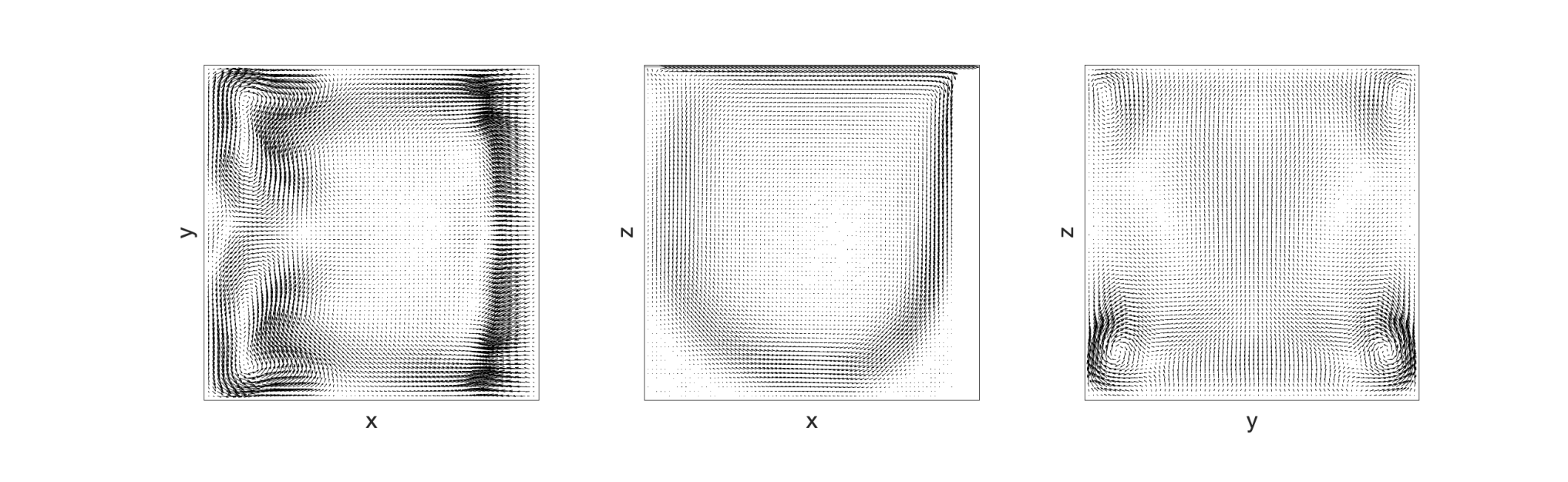
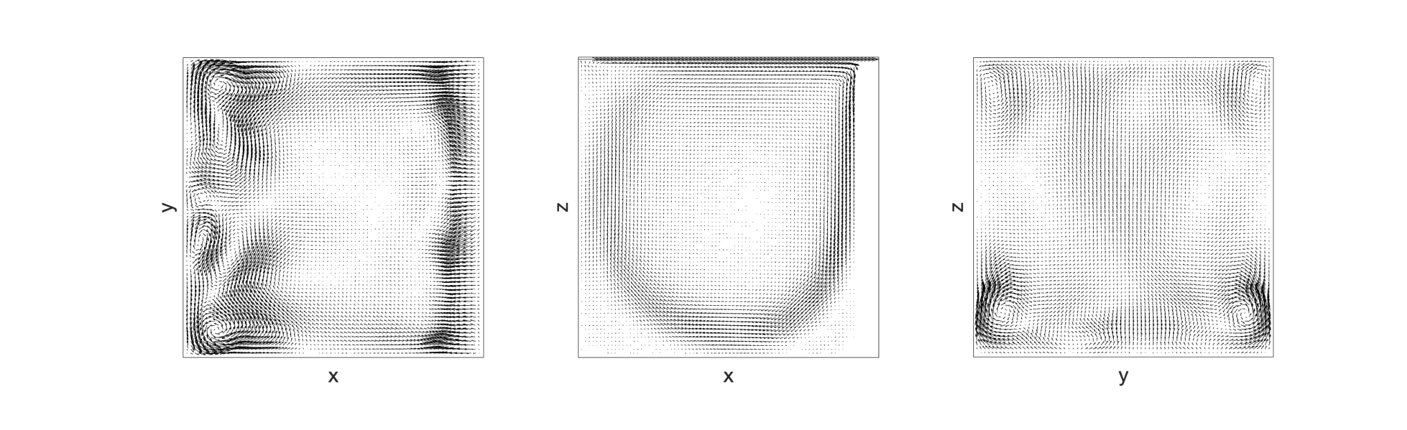
With this technique, the solver attained convergence up to (using AAPicard with and , up to a residual tolerance of , then switching to Newton with a line search). With this method, 217 iterations were needed to converge to a tolerance of in the -norm. With a continuation method that improves the initial guess, solutions at even higher can be obtained. Plots of the and solutions are shown in Figure 7 as midsliceplanes of the velocity fields.
7 Conclusion
The presented one-step analysis of Anderson acceleration sharpens the previously developed residual bounds for contractive operators and extends them to a class of potentially noncontractive operators which are important for the the approximation of solutions to nonlinear PDEs. The new analysis shows how the relative scaling of the higher-order terms increases as the solution to the underlying optimization problem improves. Understanding the balance of the higher and lower order terms in the residual expansion is instrumental in the design of robust and efficient algorithms for challenging nonlinear problems. The current theory assumes that the latest difference between consecutive residuals sufficiently changes the span of the previous differences, up to the given algorithmic depth. An efficient safeguarding strategy to ensure this assumption holds is introduced and demonstrated, advancing the connection between theory and practice in a sense not accomplished with the usual assumption that the optimization coefficients are bounded. Practical advantages based on the present advances in theory are demonstrated in the numerical section where Anderson acceleration is used to attain results for the nonlinear Helmholtz equation and 3D steady Navier-Stokes past the first Hopf bifurcation which cannot be attained by the usual combinations of Picard iterations, Newton iterations and relaxation techniques alone.
Acknowledgements
SP is partially supported by NSF DMS 1852876 and 2011519. LR is partially supported by NSF DMS 1522191 and 2011490. The authors would like to thank the anonymous referees for suggesting additional clarification on the connection between the theory and the examples, and on the value of assuming (5.4) instead the boundedness of the optimization coefficients.
References
- [1] E. Akervik, L. Brandt, D. Henningson, J. Hoepffner, O. Marxen, and P. Schlatter. Steady solutions of the Navier-Stokes equations by selective damping. Physics of Fluids, 18:1–4, 2006.
- [2] M. S. Alnæs, J. Blechta, J. Hake, A. Johansson, B. Kehlet, A. Logg, C. Richardson, J. Ring, M. E. Rognes, and G. N. Wells. The FEniCS project version 1.5. Archive of Numerical Software, 3(100), 2015.
- [3] H. An, X. Jia, and H. Walker. Anderson acceleration and application to the three-temperature energy equations. Journal of Computational Physics, 347:1–19, 2017.
- [4] D. G. Anderson. Iterative procedures for nonlinear integral equations. J. Assoc. Comput. Mach., 12(4):547–560, 1965.
- [5] G. Baruch, G. Fibich, and S. Tsynkov. High-order numerical method for the nonlinear Helmholtz equation with material discontinuities in one space dimension. Journal of Computational Physics, 227:820–850, 2007.
- [6] J. W. Both, K. Kumar, J. M. Nordbotten, and F. A. Radu. Anderson accelerated fixed-stress splitting schemes for consolidation of unsaturated porous media. Computers & Mathematics with Applications, 77(6):1479–1502, 2019. 7th International Conference on Advanced Computational Methods in Engineering (ACOMEN 2017).
- [7] C. Brezinski, M. Redivo-Zaglia, and Y. Saad. Shanks sequence transformations and Anderson acceleration. SIAM Review, 60(3):646–669, 2018.
- [8] P. R. Brune, M. G. Knepley, B. F. Smith, and X. Tu. Composing scalable nonlinear algebraic solvers. SIAM Review, 57(4):535–565, 2015.
- [9] T. Chan. An improved algorithm for computing the singular value decomposition. ACM Transactions on Mathematical Software, 8:72–83, 1982.
- [10] S.-H. Chiu, T.-W. Pan, J. He, A. Guo, and R. Glowinski. A numerical study of the transition to oscillatory flow in 3d lid-driven cubic cavity flows. 2016.
- [11] J. I. Diaz and F. De Thelin. On a nonlinear parabolic problem arising in some models related to turbulent flows. SIAM Journal on Mathematical Analysis, 25(4):1085–1111, 1994.
- [12] L. Diening, M. Fornasier, R. Tomasi, and M. Wank. A relaxed kačanov iteration for the -Poisson problem. Numer. Math., 145:1–34, 2020.
- [13] C. Evans, S. Pollock, L. Rebholz, and M. Xiao. A proof that Anderson acceleration improves the convergence rate in linearly converging fixed point methods (but not in those converging quadratically). SIAM J. Numer. Anal., 58(1):788–810, 2020.
- [14] V. Eyert. A comparative study on methods for convergence acceleration of iterative vector sequences. J. Comput. Phys., 124(2):271–285, 1996.
- [15] M. S. Fabien, M. G. Knepley, and B. M. Rivière. A hybridizable discontinuous Galerkin method for two-phase flow in heterogeneous porous media. International Journal for Numerical Methods in Engineering, 116(3):161–177, 2018.
- [16] H. Fang and Y. Saad. Two classes of multisecant methods for nonlinear acceleration. Numer. Linear Algebra Appl., 16(3):197–221, 2009.
- [17] Y. Feldman and A. Gelfgat. Oscillatory instability of a three-dimensional lid-driven flow in a cube. Phys. Fluids, 22(093602):1–9, 2010.
- [18] V. Girault and P.-A. Raviart. Finite element methods for Navier–Stokes equations: Theory and algorithms. Springer-Verlag, Berlin, Heidelberg, 1986.
- [19] R. Glowinski and J. Rappaz. Approximation of a nonlinear elliptic problem arising in a non-Newtonian fluid flow model in glaciology. ESAIM: Mathematical Modelling and Numerical Analysis, 37(1):175–186, 2003.
- [20] G. H. Golub and C. F. Van Loan. Matrix Computations (3rd Ed.). Johns Hopkins University Press, Baltimore, MD, USA, 1996.
- [21] N. Higham and N. Strabic. Anderson acceleration of the alternating projections method for computing the nearest correlation matrix. Numerical Algorithms, 72:1021–1042, 2016.
- [22] C. T. Kelley. Numerical methods for nonlinear equations. Acta Numerica, 27:207–287, 2018.
- [23] P. A. Lott, H. F. Walker, C. S. Woodward, and U. M. Yang. An accelerated Picard method for nonlinear systems related to variably saturated flow. Adv. Water Resour., 38:92–101, 2012.
- [24] Y. Peng, B. Deng, J. Zhang, F. Geng, W. Qin, and L. Liu. Anderson acceleration for geometry optimization and physics simulation. ACM Transactions on Graphics, 37(4):42:1–42:14, 2018.
- [25] S. Pollock, L. Rebholz, and M. Xiao. Anderson-accelerated convergence of Picard iterations for incompressible Navier-Stokes equations. SIAM J. Numer. Anal., 57(2):615–637, 2019.
- [26] S. Pollock and H. Schwartz. Benchmarking results for the Newton-Anderson method. Results in Applied Mathematics, 8:100095, 2020.
- [27] A. Sidi. SVD-MPE: An SVD-based vector extrapolation method of polynomial type. Applied Mathematics, 7:1260–1278, 2016.
- [28] D. A. Smith, W. F. Ford, and A. Sidi. Extrapolation methods for vector sequences. SIAM Review, 29(2):199–233, 1987.
- [29] P. Stasiak and M. Matsen. Efficiency of pseudo-spectral algorithms with Anderson mixing for the SCFT of periodic block-copolymer phases. Eur. Phys. J. E, 34:110:1–9, 2011.
- [30] A. Toth, C. Kelley, S. Slattery, S. Hamilton, K. Clarno, and R. Pawlowski. Analysis of Anderson acceleration on a simplified neutronics/thermal hydraulics system. Proceedings of the ANS MC2015 Joint International Conference on Mathematics and Computation (M&C), Supercomputing in Nuclear Applications (SNA) and the Monte Carlo (MC) Method, ANS MC2015 CD:1–12, 2015.
- [31] A. Toth and C. T. Kelley. Convergence analysis for Anderson acceleration. SIAM J. Numer. Anal., 53(2):805–819, 2015.
- [32] H. F. Walker and P. Ni. Anderson acceleration for fixed-point iterations. SIAM J. Numer. Anal., 49(4):1715–1735, 2011.
- [33] K. Wong and A. Baker. A 3d incompressible Navier-Stokes velocity-vorticity weak form finite element algorithm. International Journal for Numerical Methods in Fluids, 38:99–123, 2002.
- [34] C. Yang, J. C. Meza, B. Lee, and L.-W. Wang. KSSOLV-a MATLAB toolbox for solving the Kohn–Sham equations. ACM Trans. Math. Software, 36:1–35, 2009.
Appendix
The proof of the technical Lemma 5.3 follows.
Proof.
The proof follows by induction on the submatrix formed by the first rows and columns of , then by induction indexing up the entries of the right-most column. Let , the upper-left block of , with inverse .
The off-diagonal entries of are given by , and by Proposition 5.2 the diagonal entries are given by , following the convention that the columns of are chosen so the are positive.
For the trivial case of , , and . By Proposition 5.1, to compute the inverse of it remains to compute and . It is useful here to state the inversion formula for entries of the right-most column (index ) as
| (.1) |
For , the inversion formula (.1) and expression (5.1) for the diagonal entries yield . Then by the hypotheses of the lemma, . Using (.1), the off-diagonal entry then satisfies , yielding . Hence for the result holds. Continue by induction on , assuming the result holds for . Then for ,
Similarly by (.1), This satisfies the base step on the inner induction, up row of . Assuming the bound of (5.3) for holds for down to , it suffices to show the result for . By (.1) and the inductive hypothesis,
Setting
| (.2) |
Rearranging the terms in the sum shows
| (.3) | ||||
Applying (Proof.) and (5.1) to (.2) allows
which completes the inductive step on and hence on , and establishes the result. ∎