On Re-Balancing Self-Interested Agents in Ride-Sourcing Transportation Networks
Abstract
This paper focuses on the problem of controlling self-interested drivers in ride-sourcing applications. Each driver has the objective of maximizing its profit, while the ride-sourcing company focuses on customer experience by seeking to minimizing the expected wait time for pick-up. These objectives are not usually aligned, and the company has no direct control on the waiting locations of the drivers. In this paper, we provide two indirect control methods to optimize the set of waiting locations of the drivers, thereby minimizing the expected wait time of the customers: 1) sharing the location of all drivers with a subset of drivers, and 2) paying the drivers to relocate. We show that finding the optimal control for each method is NP-hard and we provide algorithms to find near-optimal control in each case. We evaluate the performance of the proposed control methods on real-world data and show that we can achieve between to improvement in the expected response.
I Introduction
In recent years, ride-sourcing services such as UberX and Lyft have emerged as an alternative mode of urban transportation. The reduced wait times for pickup of these services is the compelling feature compared to the conventional taxi services [1]. A key factor that affects the response time of the service is where the drivers wait to respond to the next ride request. Ride-sourcing companies do not have control over the position of the drivers as they are self-interested units maximizing their objectives. Therefore, a challenge is to ensure the drivers are distributed throughout the city in order to minimize the expected wait time of the customers. This must be done either by providing information to drivers, or through incentives (payment) that make relocation attractive.
As a method for both re-balancing and increasing the supply of drivers, Uber introduced surge pricing in high demand areas. This reduces the expected response time of servicing the requests by drawing more drivers to those areas. However, the surge pricing can draw drivers away from lower demand areas, resulting in higher wait times in those areas and more imbalance [2, 3].
The problem of servicing requests in ride-sourcing networks can be divided into two major problems: 1) assignment of the ride request to the drivers; and 2) re-balancing of the drivers for future ride requests. In this paper, we focus on the re-balancing problem for a subset of drivers to service ride requests that arrive sequentially in an environment. The drivers’ motion in the environment is captured as a road-map (i.e., graph), and each ride request arrives at a node of the graph according to a known arrival rate (see Figure 1). The drivers are self-interested units maximizing the expected profit of their workday. Hence, the ride-sourcing company has no direct control over the waiting locations of the drivers. The objective of the ride-sourcing company is to incentivize the drivers to relocate to a set of waiting locations that minimizes the expected wait-time of the customers.
Related Work: The problem of dispatching taxis to service ride requests arriving sequentially over time has been the subject of extensive research [4, 5, 6, 7]. These studies focus on policies to optimally assign the ride requests to the taxis. In contrast, we focus on the waiting locations of the drivers that minimize the expected wait time of the customers. We assume the ride requests are assigned in a first-come-first-serve fashion to the closest available driver. Assigning the closest available driver to each request is the common method employed by the ride-sourcing companies [8].

The problem of re-balancing service units in the environment has been studied for various applications. In mobility-on-demand problem (MOD) [9, 10, 11], a group of vehicles are located at a set of stations. The customers arrive at the stations, hire the vehicles for ride, and then drop the vehicles off at their destination stations. The objective is to balance the vehicles at the stations to minimize the expected wait time of the customer. In comparison to MOD, we consider the customer wait-time as the time between the request arrival and the pick-up time, which incorporates the distance of the closest available vehicle to the pick-up location.
The facility location problem [12, 13] and its extension to the mobile facility location problem (MFL) [14] is the problem of distributing facilities in a set of locations to respond to the demands arriving at different locations. The objective is to minimize the time to respond to the demands and the total cost of opening facilities. A special case of the facility location problem is the -median problem [13] where the number of open facilities is limited and the cost of opening a facility is zero. In [15], we addressed a multi-stage MFL problem where we relocate a set of autonomous vehicles to minimize expected response time for future requests in a receding horizon manner.
In the aforementioned studies, the actions of service units are controlled by a central unit and the objective of the service units is aligned with the global objective. However, we consider self-interested units maximizing their own profit such that the ride-sourcing companies have no direct control on their decisions. A closely related problem is that of Voronoi games on graphs [16] where requests arrive on the vertices of a graph and the objective of each self-interested service unit is to maximize the number vertices assigned to them. They cast the problem as a game between the service units prove that the problem of finding the pure Nash equilibrium on general graphs is NP-hard. In [17], the authors provide the best response strategy for each driver and they approximate Nash equilibria, which can be utilized by the ride-sourcing companies to incentivize the drivers in a way to maximizes a global objective. These studies focus on the strategies of the self-interested service units, in contrast, we focus on finding the optimal policy for the ride-sourcing company to optimally respond to the ride requests.
Contributions: The contributions of this paper are threefold. First, we formulate the re-balancing problem of self-interested service units. Second, we propose two indirect method to relocate the service units to minimize the expected response time and provide algorithms with near-optimal solutions. Third and finally, we evaluate the performance of the two proposed control methods on real-world ride-sourcing data.
The paper is organized as follows. In Section II, we formulate the problem of minimizing customer wait-time with self-interested service units. In Section III, we provide the first indirect control method based on sharing the information on the location of the drivers. Section IV.I consists of the second control method based on incentive pay for the drivers to relocate to desired waiting locations. Finally in Section V, we provide an extensive set of experiments, on real-world ride-sourcing data, characterizing the performance of the two control methods.
II Problem Formulation
Consider a set of drivers and a set of pick-up and drop-off locations . Let be a metric graph on vertices , let be the set of edges between the locations and be the function assigning a travel time to each edge of the graph. The drivers wait on a subset of the vertices for the next request, which we call the configuration of the drivers . The set of all configurations of the drivers is denoted by . Each driver is aware of the position of a subset of the drivers , for instance, each driver may be aware of the location of the other drivers in its vicinity.
We assume that the requests arrive at each vertex according to an independent Poisson process with arrival rate . Upon a request arrival, the closest driver to the vertex of the request is assigned to service the request. Let denote the arrival probability, which is the ratio of number of requests arriving at to the total number of requests arriving in a period of time. Let the drop-off probability be the probability that a request with pickup location at vertex has a drop-off location at vertex .
Driver ’s perception of her expected profit is a function of her information on the location of other drivers, environment parameters such as arrival times, her waiting location and the period of working time , denoted by . For the development of our main control methods we do not assume any specific form of this function. We do assume, however, that the ride-sourcing company has access to this function, obtained through data of driver behavior. In Section V we present one potential model of , which is then used for simulating the two control methods.
Drivers’ objective: Each driver is a self-interested unit, therefore, they will wait at a location that maximizes their expected profit, i.e.,
| (1) |
where is the cost per minute of driving.
Global objective: In addition to the objective of each driver, there is a global objective for the service providers such as Uber and Lyft to maximize the service quality by minimizing the expected wait time of the customers until pick-up, i.e.,
| (2) |
The main challenge in optimizing the global objective is that the drivers are self-interested units and the service provider does not have any direct control on the configuration of the vehicles. Therefore, the service provider is not able to minimize the expected response time to the requests directly. The two indirect control methods proposed in this paper incentivize the drivers to relocate to desired waiting locations. The first control method exploits the dependency of the expected profit of the drivers on their information . The service provider can share more information on the location of drivers with a subset of them to manipulate their decision towards relocating to a desired waiting location. We refer to this as the sharing information control method. The second proposed control method, incentivizes the drivers to relocate to desired waiting locations with payments, which we refer to as the pay-to-control method. These control methods are applicable to various models of driver behaviour .
In the following sections, we provide a detailed description of the two control methods and propose algorithms to find near optimal controls.
III Control by Sharing Information
In this section, we provide an indirect control on the configuration of the drivers exploiting the fact that the optimal waiting location for each driver in Equation (1) is a function of the information provided to the driver regarding the position of the other drivers, i.e., .
Figure 2 demonstrates the importance of information on an instance of the ride-sourcing problem with two vehicles and two request locations. The locations are within unit distance apart and the arrival rate at locations and are and , respectively. The vehicles are initially located at and will relocate to the best waiting location, namely optimizing Equation (1). Figure 2(a) shows the two scenarios where both vehicles are provided the same information, i.e., and . Note that the configuration of the vehicles when they are provided the same information is the worst possible configuration for the global objective. However, illustrated in Figure 2(b), providing the information to a subset of the vehicles results in the optimal configuration for the global objective.


The information sharing problem consists of deciding the subset of drivers we share information with and the information shared with each driver. However, for this work, we consider the binary decision where either full information or no information is provided.
Let (resp. ) be the new waiting location selected by driver from Equation (1) with information (resp. ). Let be the set of candidate waiting locations for driver . If there exist such that , then we create a duplicate vertex for such that for all . The formal definition of the problem of sharing information with drivers is given as follows:
Problem III.1.
Consider a metric graph . Find a new configuration by picking only one vertex from each , i.e., such that for each , while minimizing the global objective .

Figure 3 shows an instance of the information sharing problem. The green vertices are the waiting locations of the drivers if they have no information on the position of the other drivers, and the red vertices are the waiting locations of the drivers if the information is provided to each driver by the service provider. Let be the solution to Problem III.1 in which if then the driver is provided complete information of the position of the other drivers, and no information is available for driver if .
First, we analyze the complexity of Problem III.1, and then we provide an LP-rounding algorithm to find the controls.
III.I Proof of Hardness
Consider an instance of CNF-SAT with Boolean variables and clauses. We will reduce this problem to Problem III.1.
- (i)
Let contain vertices, partitioned into sets of size two. The set contains two vertices, , where will correspond to setting the th SAT variable to true (i.e., the positive literal) and will correspond to setting it to false (i.e., the negative literal).
- (ii)
We let contain vertices, one representing each clause in the SAT formula.
- (iii)
Let contain an edge for each and .
- (iv)
For each , we set its cost to if the literal appears in the clause , and if the literal does not. Note that the costs are metric.
- (v)
Let for each .
Now, we solve the instance of Problem III.1. If it returns a subset of with cost exactly , then for each clause , there is literal in with edge cost of to . This implies that the literal chosen from each subset in the partition of gives a satisfying truth assignment for the SAT instance. If the subset returned has a cost greater than , then there exists a clause for which every chosen literal has edge cost of . Thus, this clause is not satisfied and no satisfying instance exists.
III.II Linear-Program Rounding Algorithm
Given that Problem III.1 is NP-hard, we turn our focus to suboptimal algorithms. In particular, we provide a simple Linear Program (LP)-rounding algorithm for Problem III.1. Although we do not provide bound on the performance of the LP-rounding algorithm, we evaluate the performance of the algorithm on an extensive set of real-world ride sourcing data in Section V and we show that the proposed algorithm is on average within of the optimal.
First we cast Problem III.1 as an integer linear program (ILP), then we propose a rounding algorithm based on the solution to the relaxation of the ILP. Let integer parameter denote the assignment of a request at to a driver at vertex if , and otherwise. Let the integer parameter for all represent if there is a driver assigned to wait for next request arrival at . Then we write the ILP for Problem III.1 as follows:
| minimize | (3) | |||
| subject to: | (4) | |||
| (5) | ||||
| (6) | ||||
By constraint (4), a feasible solution assigns each request location to a driver. Equation (5) ensures that a request is assigned to only if there is a driver located at , and finally Equation (6) shows that in a feasible solution only one of the candidate waiting locations is chosen from each subset , which represent that either the information is provided to a driver or otherwise.
Now we propose our LP-rounding algorithm for Problem III.1. Let be the solution to the LP relaxation of ILP (3). Without loss of generality for all , let and . Given solution we construct an integer solution to ILP (3) by setting for each vertex with and . In a case, and , we set where is the optimal waiting location of driver with . Then we assign each vertex to the closest vertex in with by setting . Note that the constructed solution satisfies the constraint of ILP (3), therefore, it is a feasible solution to Problem III.1. Also, observe that the optimal objective value to the LP relaxation is a lower-bound on the optimal value of ILP (3) and provides a bound on the performance of the LP-rounding algorithm.
In the solution to the information sharing problem, if driver is selected to receive information on the location of drivers, a snapshot of the location of drivers is presented to driver and the driver can calculate their expected profit based on complete information. This method employed at each time step and presents information to a driver if there is an opportunity to improve the expected response time.
The problem of information sharing indirectly controls the configuration of the drivers by providing information to a subset of them, however, the possible configurations are limited to the candidate waiting locations of the drivers. In the following section, we provide the details on the pay-to-control method for the service provider to optimize the global objective.
IV Pay to control
Each driver as a self-interested unit chooses its waiting location by maximizing the profit in Equation (1). To convince the vehicles to relocate to another configuration, the service provider needs to compensate for the difference between their expected profit of the new location and their expected profit for the waiting location from Equation (1). First, we pose the problem between the drivers and the service provider as a game. Then we provide an approximation algorithm to find the optimal policy for the service provider.
IV.I Service Provider’s Game
Let be the incentive per unit distance offered to driver . Let (resp. ) be the configuration of the drivers before (resp. after) the incentive pay. The game between the drivers and service provider consists of the following:
- •
A set of players and a service provider,
- •
An action set for each driver , which is the waiting locations in the graph, i.e. . The action set of the service provider is ; and
- •
The profit function of the service provider is
where is a user-defined parameter that indicates the importance of the service quality for the service provider with respect to the incentive pay. For a small value of , the incentive pay is in the priority, thus the service provider will offer the waiting locations close to the driver’s desired waiting location, however, for large values of , the service provider accepts high incentive pay to relocate the drivers to the configuration with minimum expected response time.
- •
The profit of driver is the maximum of the expected profit of the offered waiting location with incentive pay and the expected profit of the waiting location from Equation (1), i.e.,
This is an instance of a leader-follower game [19]. The service provider offers an incentive based on its utility and the drivers as followers either take the offer or reject it. The service provider is aware of the best action of the drivers given any action taken by the service provider (i.e., incentive pay and the offered waiting location). The objective is to find the optimal strategy for the service provider to minimize a linear combination of the incentive pay and the expected response time by relocating the drivers to the desired configuration.
Driver will accept the offer by the service provider to relocate to only if the offered incentives surpass the best-expected profit of the driver. Since the profit functions of the drivers are known to the service provider, then the minimum in which the drivers will accept the offer to move to configuration is
| (7) |
In the equation above, is the maximum expected profit of the driver by relocating to a new waiting location, and is the expected profit of driver by waiting at the location offered by the service provider. Knowing this minimum , the objective of the service provider becomes
| (8) | ||||
Observe that is independent of the optimization parameters. Therefore, the problem of minimizing the utility function of the service provider has the mobile facility location (MFL) problem as a special case where for all and . The MFL is a well-known NP-hard problem [20] where given a metric graph , mapping and a subset of size . The objective is to find a subset minimizing
Remark IV.1 (Equilibrium).
The optimal solution to the problem is the equilibrium of the leader-follower game between the service provider and the drivers. Since any other configuration will increase the cost function of the service provider. In addition, By Equation (IV.I), waiting in a location other than the one suggested by the service provider will decrease driver’s expected profit.
IV.II Approximation Algorithm
We now propose a constant factor approximation for the minimum pay-to-control problem, namely minimizing Equation (8). Let , then the utility function of the service provider becomes
The algorithm follows by a reduction from the minimum pay-to-control problem to MFL.
Given an instance of the minimum pay-to-control problem we construct an MFL instance as follows:
- (i)
A graph where is the set of possible waiting locations for the drivers
- (ii)
There is an edge between and with cost ,
- (iii)
There is an edge between and with cost .
- (iv)
The objective is to find a set of vertices in such that minimizes

Figure 4 shows a schematic representation of the constructed MFL instance. Suppose is a solution to the MFL instance, we let be the solution of the minimum pay-to-control problem and provide the following result on the cost of the solution.
Lemma IV.2.
Given an -approximation algorithm for the MFL problem, the reduction above provides an -approximation for the minimum pay-to-control problem.
Proof.
For any , by the construction of the MFL instance, we have . Therefore, given an -approximation algorithm for the MFL problem, and obtained from the constructed MFL instance, we select as a solution to the minimum pay-to-control problem. Therefore,
V Simulation Results
We evaluate the performance of the two proposed indirect controls on ride-sourcing data from Uber [21]. The data set consists of the pick-up time and locations from April to September 2014 in New York City, primarily Manhattan. The jammed scenario occurs frequently with high demand in an area and especially when surge price is applied for the high demand area [2, 3].
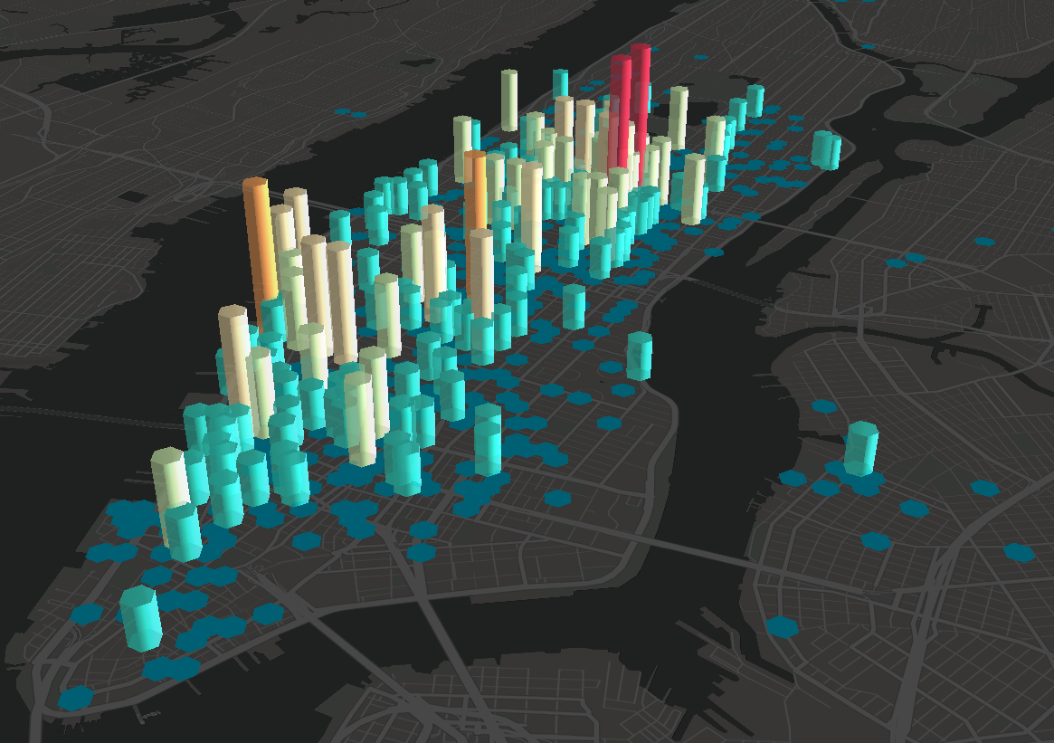
To reduce the complexity of the large data set with pick-up locations, we cluster the close pick-up locations into clusters such that no two pick-up locations in a cluster are farther than meters apart. The drop-off location for each ride is selected from the same set of clusters with equal probability. Figure 5 shows the clustered pick-up locations and the arrival rates for ride requests at each cluster is represented with a bar. The performance of the proposed control methods are evaluated in two scenarios: 1) the initial location of the drivers are selected uniformly randomly, and 2) jammed scenario where the drivers are initialized at closest locations to the Rockefeller center in Manhattan.
Observe that the proposed algorithms to find the controls are applicable to various driver models for . In the following section, we propose a behavior model for the drivers.
V.I Drivers’ model
A driver model is a process of evaluating the expected profit of different locations at each time instance. Prior to introducing our driver model, we provide the parameters in the proposed model.
The pick-up probability of a location as seen by driver is the probability that a ride-request at is assigned to driver before any other ride request. Consider a configuration of the drivers and a vertex , where driver is the th closest driver to the vertex location . Since a request is assigned to the closest available driver, then driver can expect to be assigned to the th request arriving at . Let denote the number of drivers closer to than driver located at vertex . Note that is a function of the information of driver regarding the position of other drivers. Figure 6 illustrates an instance with three vehicles and a pick-up location. Given the full information of the vehicle positions, at pick-up location is and is zero if .
The probability that a request at is assigned to driver located at as expected by driver before any other request is approximated by
Let be the fare per unit time of servicing a request, then the profit of a ride with pick-off at and drop-off at for driver located at is .


Now we define the expected profit of driver located at and working for period of time as follows:
| (9) | ||||
where for all , drivers and . Note that, represents the expected profit of driver after drop-off at . The conditional probability of the drop-off location is the common knowledge of the drivers and the ride-sourcing companies based on prior customer data.
Intuitively, the expected profit in Equation (9) represents the total expected profit of servicing requests with pick-up location at and drop-offs at only if the
Observe that finding for all and a given is performed in polynomial time, however, since the drivers are not going through the calculation of for all , we assume that they have access to the expected profit of the vertices by experience.
Since the calculation of the expected profit for drivers for each time step is computationally expensive, we trained a Random Forest Regressor [22] implemented by [23] to approximate the values of for each number of vehicles in the system with training data over instances with work-day of average length rides, fare per mile and driving cost [24].
V.II Partial Information Sharing
Figure 7 shows the percentage improvement in the expected response time for different number of vehicles using the partial information sharing control method of Section III in the two scenarios. Observe that as the number of drivers increases, the average improvement in the expected response time increases. However, with a large number of drivers randomly placed in the environment, the expected response time decreases and the possibility to further optimize it with information sharing is limited. On the other hand, in the jammed scenario where the drivers are concentrated in an area, the information sharing method improves the expected response time by on average. The information sharing method shares information on the position of the other drivers with and of the drivers in the random initial configuration and jammed scenarios, respectively. The results are the average of instances for different number of drivers and scenarios. The boxes show the first, first and third quartiles of each set of experiments. The expected response time of the solution obtained from the LP-rounding algorithm of Section III on this set of experiments is within on average of the solution of the LP relaxation of the information sharing problem. The maximum deviation from the optimal solution of the LP relaxation is .
Figure 8 shows the expected response time of a set of drivers responding to requests arriving over time with the jammed initial configuration. In this experiment, the maximum arrival rate on the vertices is per minute, therefore, we assumed that there exist enough time to relocate between the ride request arrivals. Note that the partial information method maintains a low expected response time over the course of responding to requests compared to the same set of drivers with no control input on their waiting locations. The results are an average of experiments with randomly generated requests for each experiment. The lines represent the average and shaded areas represent the first and third quartiles.
V.III Pay to Control
In this section, we evaluate the performance of the Pay-To-Control method for the two scenarios. Figure 9 illustrates the improvement in the expected response (solid lines) time and the total amount paid to the drivers (dashed lines) to relocate for different values in the random initial configuration scenario. The shaded area represents the first and third quartiles of random instances for each number of vehicles. The amount paid is proportional to the average cost of riding UberXL, i.e., per minute [24]. For larger , the expected response time is more important than the amount paid for relocation. Therefore, with a larger number of vehicles, the Pay-To-Control method increases the amount paid to the drivers to minimize the expected response time. Notice that with the expected response time has improved by for per driver.
Next, we evaluate the performance of the pay-to-control algorithm in the jammed scenario. Figure 10 shows that with a larger number of vehicles concentrated in a small area, the pay-to-control algorithm improves the expected response time significantly with limited amounts paid to the drivers. Notice that with the expected response time has improved by for per driver.
Figure 11 shows the expected response time and the amount paid to a set of drivers responding to requests arriving over time with the jammed initial configuration. Notice that the Pay-To-Control method with maintains a low expected response time over the course of responding to requests compared to the same set of drivers with no control input on their waiting locations. The total amount paid to the drivers over the course of responding to requests is per request. The results are an average of experiments with randomly generated requests for each experiment. The lines represent the average and shaded areas represent the first and third quartiles.
VI Conclusion
This paper considered the problem of controlling self-interested drivers in ride-sourcing applications. Two indirect control methods were proposed and for each, a near-optimal algorithm was presented. The extensive results show significant improvement in the expected response time on real-world ride-sourcing data. In addition, we hope to extend the results to capture vehicles with different capacities and ride-sharing applications.
References
- [1] L. Rayle, S. Shaheen, N. Chan, D. Dai, and R. Cervero, “App-based, on-demand ride services: Comparing taxi and ridesourcing trips and user characteristics in san francisco university of california transportation center (uctc),” University of California, Berkeley, United States, 2014.
- [2] N. Diakopoulos. How Uber surge pricing really works. [Online]. Available: https://www.washingtonpost.com/news/wonk/wp/2015/04/17/how-uber-surge-pricing-really-works/
- [3] A. Rosenblat and L. Stark, “Algorithmic labor and information asymmetries: A case study of Uber’s drivers,” International Journal Of Communication, 2016.
- [4] W. Zhang, S. Guhathakurta, J. Fang, and G. Zhang, “The performance and benefits of a shared autonomous vehicles based dynamic ridesharing system: An agent-based simulation approach,” in Transportation Research Board 94th Annual Meeting, no. 15-2919, 2015.
- [5] M. Hyland and H. S. Mahmassani, “Dynamic autonomous vehicle fleet operations: Optimization-based strategies to assign AVs to immediate traveler demand requests,” Transportation Research Part C: Emerging Technologies, vol. 92, pp. 278–297, 2018.
- [6] M. Chang, D. S. Hochbaum, Q. Spaen, and M. Velednitsky, “DISPATCH: an optimal algorithm for online perfect bipartite matching with i.i.d. arrivals,” CoRR, vol. abs/1805.02014, 2018.
- [7] M. Maciejewski, J. Bischoff, and K. Nagel, “An assignment-based approach to efficient real-time city-scale taxi dispatching,” IEEE Intelligent Systems, vol. 31, no. 1, pp. 68–77, 2016.
- [8] Uber. Driving with Uber, wait less, earn more. [Online]. Available: https://www.uber.com/info/get-trips-without-waiting/
- [9] M. Pavone, S. L. Smith, E. Frazzoli, and D. Rus, “Robotic load balancing for mobility-on-demand systems,” The International Journal of Robotics Research, vol. 31, no. 7, pp. 839–854, 2012.
- [10] M. Tsao, R. Iglesias, and M. Pavone, “Stochastic model predictive control for autonomous mobility on demand,” arXiv preprint arXiv:1804.11074, 2018.
- [11] G. C. Calafiore, C. Novara, F. Portigliotti, and A. Rizzo, “A flow optimization approach for the rebalancing of mobility on demand systems,” in IEEE International Conference on Decision and Control, 2017, pp. 5684–5689.
- [12] D. B. Shmoys, “Approximation algorithms for facility location problems,” in International Workshop on Approximation Algorithms for Combinatorial Optimization. Springer, 2000, pp. 27–32.
- [13] V. Arya, N. Garg, R. Khandekar, A. Meyerson, K. Munagala, and V. Pandit, “Local search heuristics for k-median and facility location problems,” SIAM Journal on computing, vol. 33, no. 3, pp. 544–562, 2004.
- [14] E. D. Demaine, M. Hajiaghayi, H. Mahini, A. S. Sayedi-Roshkhar, S. Oveisgharan, and M. Zadimoghaddam, “Minimizing movement,” ACM Transactions on Algorithms (TALG), vol. 5, no. 3, p. 30, 2009.
- [15] A. Sadeghi and S. L. Smith, “Re-deployment algorithms for multiple service robots to optimize task response,” in IEEE International Conference on Robotics and Automation, 2018, pp. 2356–2363.
- [16] S. Bandyapadhyay, A. Banik, S. Das, and H. Sarkar, “Voronoi game on graphs,” Theoretical Computer Science, vol. 562, pp. 270–282, 2015.
- [17] R. Salhab, J. Le Ny, and R. P. Malhamé, “A dynamic ride-sourcing game with many drivers,” in 55th Annual Allerton Conference on Communication, Control, and Computing, 2017, pp. 770–775.
- [18] R. Schuler, “An algorithm for the satisfiability problem of formulas in conjunctive normal form,” Journal of Algorithms, vol. 54, no. 1, pp. 40–44, 2005.
- [19] T. Basar and G. J. Olsder, Dynamic noncooperative game theory. Siam, 1999, vol. 23.
- [20] S. Ahmadian, Z. Friggstad, and C. Swamy, “Local-search based approximation algorithms for mobile facility location problems,” in Proceedings of the twenty-fourth annual ACM-SIAM symposium on Discrete algorithms. SIAM, 2013, pp. 1607–1621.
- [21] (2014) Uber TLC FOIL response. [Online]. Available: https://github.com/fivethirtyeight/uber-tlc-foil-response
- [22] L. Breiman, “Random forests,” Machine learning, vol. 45, no. 1, pp. 5–32, 2001.
- [23] F. Pedregosa, G. Varoquaux, A. Gramfort, V. Michel, B. Thirion, O. Grisel, M. Blondel, P. Prettenhofer, R. Weiss, V. Dubourg, J. Vanderplas, A. Passos, D. Cournapeau, M. Brucher, M. Perrot, and E. Duchesnay, “Scikit-learn: Machine learning in Python,” Journal of Machine Learning Research, vol. 12, pp. 2825–2830, 2011.
- [24] Ride sharing driver. How much does uber cost? Uber fare estimator. [Online]. Available: https://www.ridesharingdriver.com/